Cascade Extended State Observer
for Active Disturbance Rejection Control
Applications under Measurement NoiseJournal: ISA Transactions
Abstract
The extended state observer (ESO) plays an important role in the design of feedback control for nonlinear systems. However, its high-gain nature creates a challenge in engineering practice in cases where the output measurement is corrupted by non-negligible, high-frequency noise. The presence of such noise puts a constraint on how high the observer gains can be, which forces a trade-off between fast convergence of state estimates and quality of control task realization. In this work, a new observer design is proposed to improve the estimation performance in the presence of noise. In particular, a unique cascade combination of ESOs is developed, which is capable of fast and accurate signals reconstruction, while avoiding over-amplification of the measurement noise. The effectiveness of the introduced observer structure is verified here while working as a part of an active disturbance rejection control (ADRC) scheme. The conducted numerical validation and theoretical analysis of the new observer structure show improvement over standard solution in terms of noise attenuation.
Keywords:
high-gain observers , noise filtering , active disturbance rejection control , ADRC , extended state observer , ESO1 Introduction
A common strategy in the class of active disturbance rejection control (ADRC [1, 2]) techniques for extracting otherwise unavailable information about the governed system is to use an extended state observer (ESO). It simultaneously provides information about the missing state variables (required for controller synthesis) as well as the lumped disturbances/uncertainties (also denoted as total disturbance [3]). Successful deployments of ADRC have been well documented in various control areas including process [4, 5], power [6, 7], and motion [8, 9, 10, 11, 12, 13] control. The effectiveness of the ADRC methodology has been also validated theoretically addressing its applicability to linear time-invariant (LTI) [14] and nonlinear time-variant (NTV) [15, 16] systems by using various tools like Lyapunov [17] and singular perturbation techniques [18]. A recent review [19] covers standard and new theoretical achievements in ADRC for uncertain finite-dimensional and infinite-dimensional systems. To date, different ESO architectures have been proposed and tested to address specific control problems (e.g. [20, 21]). The motivation for studying ADRC also comes from the fact that it is one of just few class of control approaches that was successfully transitioned from academia to industry on a significant scale and is being used in commercial motion and process control products (e.g. from Danfoss, Texas Instruments).
To a large extent, the performance of any ADRC scheme relies on the speed and accuracy of the ESO. It is well-known that high-gain observers (including ESO) are robust against model uncertainty and disturbances. However, the theory of observers also reveals the existence of a trade-off between speed/accuracy of state reconstruction and sensitivity to high-frequency measurement noise [22]. The adverse, non-negligible effects of measurement noise are omnipresent in engineering practice and can be found in various important applications, including fuel cells [23], magnetic levitation-based transportation [24], water management systems [25], and aerial vehicles [26]. The sensor noise is also an important factor in the design of effective adaptive algorithms including adaptive controllers [27] and adaptive parameter estimators [28]. Hence, the problem of noise is still an active research topic with different solutions proposed to attenuate the effects of measurement noise to date. They mainly address the problem by: employing nonlinear [1, 29] or adaptive techniques [30, 31, 32], redesigning the local behavior by combining different observers [33, 34, 35, 36], employing low-power structures [37, 38, 39, 40], increasing the observer order with integral terms [41, 42], adding special saturation functions [43], or modifying standard low-pass filters [44, 45].
The above techniques, although suitable for certain control scenarios, in general, may encounter several limitations from theoretical and/or practical point of view. Such limitations include complicated implementation (nonlinear techniques), additional assumptions of persistent excitation of certain signals (adaptive techniques), extra knowledge requirement for the design and tuning of additional components (combination of different observers), increased noise attenuation but reduced signal convergence speed (low-power structures), introduction of nonlinear components in the design which complicate its theoretical analysis and practical implementation (saturation functions), and introduction of extra system lag (modifications of standard low-pass filters).
Motivated by the above limitations and the practical importance of an effective denoising algorithm in nonlinear feedback control, in this work, a new paradigm to redesign high-gain observers is proposed in order to improve their performance in the presence of measurement noise. It directly addresses the limitations posed by the trade-off between speed/accuracy of state estimation and noise sensitivity. The principle behind the proposed approach is based on a decomposition of the unknown total disturbance into a predefined number of parts, each representing certain signal frequency range, and reconstruction of the decomposed parts with a set of cascaded observers. In contrast to a standard, single-observer ADRC, the introduced multi-observer topology allows to use higher observer bandwidths for reconstructing signals with smaller sensor noise impact. Hence, the contribution of this work is a proposition of the new cascade ESO topology, which is capable of providing fast and accurate estimates while avoiding over-amplification of the sensor noise and retaining the relatively straightforward implementation. To the best of our knowledge, such design is presented for the first time in the context of current literature.
Notation. Throughout this paper, we use as a set of real numbers, as a set of positive real numbers, as a set of integers, while and represent zero and identity matrices of the appropriate order, respectively. Relation means that is positive-definite, corresponds to the Euclidean norm of the vector , is a matrix norm defined as , while and correspond to the minimal and maximal eigenvalues of matrix . Set represents a class of locally Lipschitz continuously differentiable functions, while is a class of strictly increasing functions with the zero-value at the origin.
2 Preliminaries: standard ESO
Before the proposed cascade ESO is explained, theoretically proven, and finally validated in a numerical simulation, let us first recall the standard ESO and highlight its limitations when used in noisy environments. First, a nonlinear dynamical system is represented by the state-space model
| (1) |
where is a system state, is an external disturbance, is a control signal, is a system output, corresponds to the measurement noise, describes the influence of the control signal on the system dynamics, represents lumped dynamics of the controlled plant, time , while is a known order of the dynamical system, , , and .
Assumption 1
System (1) is defined on an arbitrarily large bounded domain for , such that .
Assumption 2
Measurement noise is bounded in the sense that there exists a bounded set for some , such that .
Assumption 3
External disturbance , and , for some bounded sets and , for some .
Assumption 4
Fields and are continously differentiable locally Lipschitz functions, i.e., .
Assumption 5
Utilized control input , and for some .
State dynamics, taken from (1), can be rewritten as
| (2) |
where is the so-called total disturbance, and is a rough, constant estimate of .
Remark 1
If the mathematical model of system (1) is known, the system input gain can be straightforwardly calculated. If not, an approximated value of can still suffice as ADRC is robust (to some extent) against parametric uncertainty. The necessary and sufficient condition for the uncertain design parameter has been established in [46].
The standard ESO design, see e.g. [47], is expressed by the dynamics of the extended state estimate , i.e.,
| (4) |
where is the observer gain vector dependent on the coefficients for and on the parameter . Observation error can be defined as , while its dynamics, derived upon (3) and (4), can be expressed as
| (5) |
Remark 2
For the sake of notation conciseness of further analysis, we propose to choose the values of in a way to obtain matrix with all eigenvalues equal to .
Remark 3
Assumptions 1-5 imply bounded values of the total disturbance , and its derivative for , where . The need to ensure bounded values of , interpreted as the perturbation of the observation error system (5), is a well-known characteristics of the disturbance-observer-based controllers, recently discussed in depth in [3]. This limitation has been extensively discussed in the area of the ADRC techniques to date. Latest theoretical developments in the field have shown under what conditions (which turn out not to be difficult to satisfy in practice) it can be proved that the total disturbance and its consecutive time-derivatives will remain bounded even if it is a function of system states. This property is satisfied with the control input having a sufficiently large upper bound (see [48]), what was imposed by Assumption 5. Additionally, when a system state is within some bounded set, imposed by Assumption 1, the boundedness of state-dependent disturbance is satisfied (see [49]).
Now, in order to show the influence of total disturbance and measurement noise on the observation errors for standard ESO, let us first introduce a linear change of coordinates , where and , resulting in the transformation of (5) to
| (6) |
where
| (7) |
We propose a Lyapunov function candidate , limited by , where is the solution of Lyapunov equation
| (8) |
The derivative of , derived upon (6), can be expressed as
| (9) |
for . The derivative of holds
| (10) |
where is a chosen majorization constant and the conservatively estimated lower bound of is a class function with respect to arguments and . According to the result (10), Assumption 2, and Remark 3, we can claim that system (6) is input-to-state stable11 1 The definition and selected properties of input-to-state stable system are described in the Appendix A. (ISS) with respect to perturbations and , and satisfies
| (11) |
for . To achieve the minimal asymptotic upper-bound of the transformed observation error , we need to find a trade-off between the reduction of impact with the increasing values and the influence of amplified by . It is worth noting, that for the nominal case when and , the asymptotic upper bound of , implying the asymptotic upper bound of the original observation error vector . In the case of non-zero values of and , as and .
Remark 4
Since in the practical conditions the value of parameter , inequality implies that the asymptotic relation (11) and all of the further comments hold also for the original observation error .
3 Main result: cascade ESO
3.1 Concept
Following [2], the concept of ADRC relies on the feedforward cancellation of the total disturbance included in the generic controller
| (12) |
where represents the new virtual control signal, most commonly in the form of a stabilizing feedback controller. After the application of control signal into dynamics (2), one can observe that the first component of (12), i.e. , should cancel out the total disturbance , while the second component, i.e. , is responsible for pushing the state vector towards the desired reference value.
Remark 5
To keep the article focused on the design of cascade ESO, we do not introduce nor analyze here any specific feedback controller . At this point, we assume that is some bounded and locally Lipschitz function consistent with Assumption 5, that assures the asymptotic convergence of system state to its reference value for the ideal case, when and .
Substitution of (12) into the dynamics (2) results in the closed-loop form of the considered system expressed as
| (13) |
where is the residual total disturbance. Let us now assume that the parameter of the standard ESO, see (4), was set to a relatively low value which only allows a precise following of the first element of extended state, i.e. , but filters out the measurement noise . Latter elements of the extended state are dependent on the further derivatives of the first one, and usually are more dynamic and have faster transients, thus are not estimated precisely by ESO using chosen . As a consequence, values of the total disturbance residue can be substantial causing a possible loss of control precision.
To improve the estimation performance of the extended state obtained with the standard ESO with low , treated here as a first level in the cascade observer structure, let us introduce the state vector of the second level of the observer , where for is the estimate of -th derivative of , while is the estimated value of residual total disturbance. The structure of the second observer level is
| (14) |
where and , . Furthermore, by substituting the virtual control signal in the above equation with (calculated upon (12)), one obtains
| (15) |
where results from the estimates of total disturbance obtained with the first cascade level (4). Note that the equation of the second observer level does not depend on the system output , thus is not affected by the measurement noise directly. The estimate of total disturbance utilized in (12) should be now taken from the new extended state estimate
| (16) |
A block diagram of the ADRC control structure with the proposed cascade ESO (for ) applied to the system (1) is shown in Fig. 1.
Remark 6
Coefficients of the cascade observer can differ in general between the cascade levels, but for the sake of notation clarity, we assume within this article that they are equal.
Remark 7
The idea of the cascade observer topology is to estimate the total disturbance observation residue resulting from the previous level with the next cascade level of ESO, implying that the observer bandwidth multiplier
The observation error, associated with the cascade observer with two levels, can be defined as
| (17) |
with its dynamics derived upon (15), (4), and (3) as
| (18) |
for , and .
Following the reasoning presented in Sect. 2 for standard ESO, we now prove that the observation error is bounded, despite a perturbing impact of total disturbance and measurement noise. Let us introduce a linear change of coordinates for , and . The dynamics of is described by
| (19) |
for matrix taken from (7). Let us introduce a Lyapunov function candidate in the form , limited by , where is a solution of the Lyapunov equation (8). The derivative of , calculated with (19), has the form
| (20) |
which holds
| (21) |
where is a chosen majorization constant and the conservatively estimated lower bound of the transformed observation error is a class function with respect to the arguments and . According to the result (21) and the definition of ISS property described in Appendix A, system (19) satisfies the asymptotic relation
| (22) |
for having the same values as the ones from (11). Summarizing, the transformed observation error is bounded in general, as and when , and when both and . Similarly to the issue described in Remark 4 for the single-stage observer, the original observation error for the second-level cascade observer () satisfies , and thus holds the ISS property itself. The obtained result presents practical stability achieved for the non-zero measurement noise and total disturbance derivative which are the perturbations of the analyzed system.
3.2 General design
In the general case, we may continue the procedure of estimating residual observation errors by increasing the level of observer cascade to the arbitrarily chosen value such that and . The cascade observer with levels can be written down as
| (23) |
for and for . The estimate of total disturbance implemented in (12) can be taken from the new extended state estimate expressed as
| (24) |
A block diagram of the ADRC control structure with the proposed cascade ESO (in its general form ) for the system (1) is shown in Fig. 2.
The observation error for the -level cascade ESO is defined as
| (25) |
with the dynamics expressed (after some algebraic manipulations made according to (3), and (23)) as
| (26) |
for , , , and . Using the linear change of coordinates for and , we may rewrite the observation error dynamics concerning -th level structure as
| (27) |
To prove the boundedness of observation errors in the general case of cascade ESO, let us propose a Lyapunov function candidate defined as and bounded by , where is a solution of an algebraic Lyapunov equation (8). The derivative of is calculated upon (27) and takes the form
| (28) |
that holds
| (29) |
According to the ISS property, steady-state values of the transformed observation error are limited by
| (30) |
where is taken from (11). Due to the recursive character of the obtained asymptotic relation and the result (11), we may also write that for some positive constants dependent on the parameters and . As it was presented for previously described observer structures, transformed observation error is generally bounded, as and when , and when both and . Similarly to the issue described in Remark 4 for the single-level observer structure, the original observation error for the -level cascade observer and thus holds the ISS property itself. The obtained result presents the practical stability achieved for the non-zero measurement noise and total disturbance derivative which are the perturbations of the analyzed system.
4 Numerical verification
4.1 Generic example
Methodology
In order to evaluate the effectiveness of the proposed cascade ESO-based ADRC design (Sect. 3) in terms of control objective realization and measurement noise attenuation, its results are quantitatively compared with the results from a standard, single ESO-based ADRC design (Sect. 2). For the purpose of this case study, a following second order time-varying single-input single-output system in form of (1) is considered:
| (31) |
with , , and . The core linear dynamics of (31) is affected (starting at s) by an external, nonlinear disturbance . The control objective is to make the output track a desired trajectory in the presence of measurement noise and despite the influence of . Signal here is a step function, additionally filtered by a stable dynamics to minimize the observer peaking. The control action is defined the same for all tested cases as in (12), with . The utilized control design is a well-known structure, studied in details for example in [18]. To keep the conciseness of notation, we treat the standard ESO as the case with . Two comparison tests are performed.
Sim1A: trajectory tracking without measurement noise
In order to establish a fair base for further comparison in the presence of measurement noise, similar performance between the tested control designs is achieved first in the idealized, noise-less conditions (). Since total disturbance estimation is the key element in any ADRC approach, the focus here is on providing similar reconstruction quality of in terms of minimizing integral criterion , with being the total disturbance observation error taken from , s being the integration start time and s being its finish time. Since the tested control algorithms do not share similar observer structure, nor have the same number of tuning parameters, it is arbitrarily decided to use a tuning methodology of single observer bandwidth parameterization from [47], which is based on a standard pole-placement procedure (cf. Remark 2). The heuristically selected observer bandwidths from Table 1 provide similar total disturbance reconstruction quality among the tested algorithms, as confirmed by Table 2. Two integral criteria are additionally introduced to evaluate overall tracking accuracy () and energy usage (), with being the feedback error.
| Observer type | Observer bandwidth |
|---|---|
| Standard ESO =1 | |
| Proposed ESO =2 | , |
| Proposed ESO =3 | , , |
| Test | Observer type | Criterion | ||
|---|---|---|---|---|
| Sim1A | Standard ESO =1 | 19.525 | 79.076 | 0.956 |
| Proposed ESO =2 | 12.351 | 89.958 | 0.957 | |
| Proposed ESO =3 | 8.346 | 84.804 | 0.955 | |
| Sim1B | Standard ESO =1 | 19.738 | 193.93 | 8.785 |
| Proposed ESO =2 | 12.833 | 100.61 | 3.162 | |
| Proposed ESO =3 | 8.952 | 93.67 | 3.006 | |
Sim1B: trajectory tracking with measurement noise
This time, a more realistic scenario is considered in which the output measurement noise is present (i.e. ), hence the only change with respect to test Sim1A is the introduction of the band-limited white noise with power . The sampling frequency is set to Hz.
Results
The results of Sim1A are gathered in Fig. 3. The selected observer bandwidths provide visually comparable results of total disturbance estimation error and energy consumption in all tested control designs, even though both cascade ESO-based designs have significantly lower observer bandwidths than standard approach. The proposed cascade ESO structures also improve the tracking quality despite having lower observer bandwidths. The observation error differs among tested techniques noticeably, however, it is expected result since in the cascade observer design, the importance of output signal estimation is being shifted and favors total disturbance estimation instead. It is done deliberately and has practical justification as it is often the case that the output signal is available directly through measurement, hence its close estimation would be redundant.
The results of Sim1B are gathered in Fig. 4. One can see that despite the presence of the measurement noise visible on zooms embedded in the plot presenting the output signal, the cascade ESO provides improvement in the noise attenuation over standard ESO, especially in the quality of total disturbance reconstruction and, consequently, in the control signal profile (Table 2). With the extra layer of cascade (), the amplitude of noise is further reduced. It is not surprising since with the increase of cascade level, lower observer bandwidths can be selected for estimating signals contaminated with high-frequency noise (hence noise is not over-amplified). At the same time, high observer bandwidths can be selected for estimating signals which are affected by the noise to a smaller extent, hence high tracking capabilities can be retained.


Additionally, Fig. 5 shows a relative quality of a total disturbance estimation, understood as the difference of criteria between the standard and proposed ESO-based designs in tests Sim1A (left) and Sim1B (right). The blue color represents area where the total disturbance is estimated more precisely with ESO associated with the horizontal axis, while the red color represents the area where an ESO structure related to the vertical axis provides better estimation. The dashed lines in the left-hand side figures connect points with equal values of estimation precision, i.e., cases having similar convergence speed of observation error. Black dots placed on each plot are representing the parameter values utilized in the simulations illustrated in time-domain in Fig. 3 and Fig. 4. When the same dashed line is plotted in the right-hand side figure associated with the comparison of standard ESO and the proposed one (both for and ), it is surrounded by blue area for high observer bandwidths () of standard ESO. This confirms numerically that the use of cascade ESO is justified when high observer gains are demanded, as it can improve the estimation precision (connected with noise attenuation) for similar convergence speed. The comparison of cascaded ESO structures for and shows that in the presence of measurement noise, the estimation quality is (a) equal for both structures, when the dashed line lays on the border of blue and red area, (b) better for level structure for a small range of relatively low values of when the dashed line is on the red area, and (c) more precise for level cascade ESO in the case of dashed line laying on the blue area. However, case with revealed (expectedly) that there is a limit to the cascade level increase. And although it is shown through the obtained numerical results that the introduction of cascade ESO structure can be beneficial in sensor noise suppression, both the specific value of and the ESO gains should be tailored on a case-by-case basis. General methodology for selection and observer tuning is still an open question.
4.2 PVTOL aircraft example
Methodology
In relation to the generic example presented in Sect. 4.1, this time, a more realistic model of a planar vertical take-off and landing (PVTOL) aircraft is considered for the verification of the proposed cascade ESO-based ADRC. According to [26], a PVTOL aircraft dynamics can be well approximated with a simplified and normalized model
| (32) | ||||
where is the normalized position and orientation vector, are the control signals corresponding to a normalized thrust and momentum of the PVTOL platform, while are the normalized signals describing the impact of crosswind, treated here as an input-additive external disturbance. We assume here that the only measurable signals are and .
In order to express system (32) in the form of (2), dynamics of the vehicle position is expressed as a 4-th order system
| (33) |
where . Using the controller equations developed in [26], defined as
| (34) |
we can rewrite system (33) as two separate subsystems with the structure given by (2), i.e.,
| (35) |
For the subsystem concerning coordinate , we can specify the assignments , and for the coordinate , assignments . Now, total disturbances associated with particular subsystems take the form of
| (36) |
The control action for each subsystem is defined for all tested cases as in (12), with , and . The desired trajectory for subsystem concerning coordinate is , while for subsystem concerning coordinate , the desired trajectory is . The initial position and orientation values are , , , their derivatives are initially set to zero, while , and . The crosswind impact is modeled as , . For the sake of a clear presentation of further results, we introduce symbols , , and for that respectively correspond to the control error , the estimate of total disturbance , and the total disturbance estimation error in a particular subsystem.
Similarly to the testing procedure utilized for the generic example in Sect. 4.1, the performance of the proposed cascade ESO-based ADRC is compared with a standard, single ESO-based ADRC. Analogously, two following tests are performed.
Sim2A: trajectory tracking without measurement noise
Similar tuning procedure to the one used in Sect. 4.1 is applied to tune the observer parameters. The heuristically selected observer bandwidths (gathered in Table 3) provide similar total disturbance reconstruction quality among the tested algorithms, as confirmed by the values of presented in Table 4. Since in the considered PVTOL aircraft control problem the initial conditions are relatively far from the reference trajectory, the integral quality indices from Table 4 are calculated for parameters s and s to avoid integration during the initial peaking of the observer states.
| Observer type | Observer bandwidth |
|---|---|
| Standard ESO =1 | |
| Proposed ESO =2 | , |
| Proposed ESO =3 | , , |
| Test | Observer type | Criterion | ||
|---|---|---|---|---|
| Sim2A | Standard ESO =1 | 3.237 | 44.508 | 0.122 |
| Proposed ESO =2 | 3.092 | 44.525 | 0.122 | |
| Proposed ESO =3 | 2.990 | 44.552 | 0.122 | |
| Sim2B | Standard ESO =1 | 3.237 | 27813 | 1121 |
| Proposed ESO =2 | 3.092 | 45.244 | 4.562 | |
| Proposed ESO =3 | 2.990 | 44.643 | 1.601 | |
Sim2B: trajectory tracking with measurement noise
In this test, the only change with respect to simulation Sim2A is an introduction of the band-limited white noise with power . The sampling sampling frequency is set to 1kHz.
Results
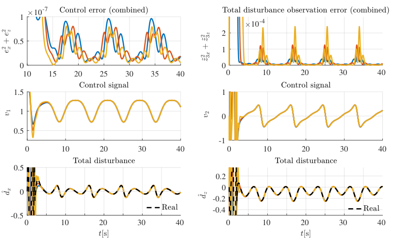
The results of the noiseless case Sim2A are gathered in Figs. 6 and 7. Even though a more complex system has been used here, comparing to the one from Sect. 4.1, similar observations can be made. Despite the fact that the cascade ESO-based designs (i.e. for and ) have significantly lower observer bandwidths than standard approach, all of the tested observer structures provide visually comparable results of the total disturbance estimation error and energy consumption.
The outcomes of the noisy case Sim2B are presented in Figs. 8 and 9. From the obtained results, one can notice that despite the presence of measurement noise visible on zooms embedded in the plot presenting the control errors and in Fig. 8, the proposed cascade ESO provides improvement in the noise attenuation over standard ESO, especially in the quality of total disturbance reconstruction and, consequently, in the control signal . With the extra layer of cascade (), the amplitude of noise is further reduced. The measurement noise does not visually impact signal , since it origins from the doubly integrated signals and , as seen in (34).



5 Conclusions
From the obtained results, one can deduce that the compromise between speed/accuracy of state reconstruction and noise amplification is still present, however, with the cascade ESO one gains extra degree of freedom in designing high-bandwidth observers while minimizing the amplification of output noise. This reveals great practical potential of the proposed method in high-performance control of systems subjected to non-negligible measurement noise. The potential drawbacks of the proposed cascade ESO-based design (like extra tuning parameters, lack of a systematic method of cascade level selection and cascade ESO tuning) need to be further investigated.
Appendix A Input-to-State (ISS) stability
Following work [50], Definition 4.7 from [51] and Assumption 12.3 from [52], a following system
| (37) |
defined on , , , and is locally input-to-state stable (ISS) on some bounded sets if there exists a function of class , and functions , of class , such that for any initial conditions and any bounded inputs , , solution exists for all , satisfying
| (38) |
and implying the asymptotic relation
| (39) |
According to Theorem 4.19 from [51], if the continuously differentiable function satisfies
| (40) |
for some -class functions and , and
| (41) |
for a continuous positive-definite function , and a class functions , then, system (37) is locally ISS with respect to the inputs and , satisfying (39) for functions , and .
References
- [1] J. Han, From PID to Active Disturbance Rejection Control, IEEE Transactions on Industrial Electronics 56 (3) (2009) 900–906.
- [2] Z. Gao, On the centrality of disturbance rejection in automatic control, ISA Transactions 53 (4) (2014) 850–857.
- [3] S. Chen, W. Bai, Y. Hu, Y. Huang, Z. Gao, On the conceptualization of total disturbance and its profound implications, Science China Information Sciences 63 (2) (2020) 129201.
- [4] Z. Wu, D. Li, Y. Xue, L. Sun, T. He, S. Zheng, Modified active disturbance rejection control for fluidized bed combustor (in press), ISA Transactions.
- [5] L. Sun, D. Li, K. Hu, K. Y. Lee, F. Pan, On tuning and practical implementation of active disturbance rejection controller: A case study from a regenerative heater in a 1000 MW power plant, Industrial & Engineering Chemistry Research 55 (23) (2016) 6686–6695.
- [6] L. Sun, Q. Hua, D. Li, L. Pan, Y. Xue, K. Y. Lee, Direct energy balance based active disturbance rejection control for coal-fired power plant, ISA Transactions 70 (2017) 486–493.
- [7] L. Dong, Y. Zhang, Z. Gao, A robust decentralized load frequency controller for interconnected power systems, ISA Transactions 51 (3) (2012) 410–419.
- [8] K. Łakomy, M. M. Michałek, Robust output-feedback VFO-ADR control of underactuated spatial vehicles in the task of following non-parametrized paths, European Journal of Control, doi:https://doi.org/10.1016/j.ejcon.2020.07.006.
- [9] R. Patelski, P. Dutkiewicz, On the stability of ADRC for manipulators with modelling uncertainties, ISA Transactions 102 (2020) 295–303.
- [10] Y. Huang, J. Su, Output feedback stabilization of uncertain nonholonomic systems with external disturbances via active disturbance rejection control, ISA Transactions.
- [11] R. Madonski, M. Kordasz, P. Sauer, Application of a disturbance-rejection controller for robotic-enhanced limb rehabilitation trainings, ISA Transactions 53 (4) (2014) 899–908.
- [12] M. M. Michałek, K. Łakomy, W. Adamski, Robust output-feedback cascaded tracking controller for spatial motion of anisotropically-actuated vehicles, Aerospace Science and Technology 92 (2019) 915–929.
- [13] A. Merola, C. Aguilar-Ibanez, H. Sira-Ramirez, M. S. Suarez-Castanon, A linear active disturbance rejection control for a ball and rigid triangle system, Mathematical Problems in Engineering 1358930.
- [14] W. Xue, Y. Huang, Performance analysis of active disturbance rejection tracking control for a class of uncertain LTI systems, ISA Transactions 58 (2015) 133–154.
- [15] S. Chen, Z. Chen, On active disturbance rejection control for a class of uncertain systems with measurement uncertainty (early access), IEEE Transactions on Industrial Electronics (2020) 1–1.
- [16] W. Xue, Y. Huang, Performance analysis of 2-DOF tracking control for a class of nonlinear uncertain systems with discontinuous disturbances, International Journal of Robust and Nonlinear Control 28 (2018) 1456–1473.
- [17] C. Aguilar-Ibanez, H. Sira-Ramirez, J. A. Acosta, Stability of active disturbance rejection control for uncertain systems: A Lyapunov perspective, International Journal of Robust and Nonlinear Control 27 (18) (2017) 4541–4553.
- [18] S. Shao, Z. Gao, On the conditions of exponential stability in active disturbance rejection control based on singular perturbation analysis, International Journal of Control 90 (10) (2017) 2085–2097.
- [19] Z.-H. Wu, H.-C. Zhou, B.-Z. Guo, F. Deng, Review and new theoretical perspectives on active disturbance rejection control for uncertain finite-dimensional and infinite-dimensional systems, Nonlinear Dynamics.
- [20] K. Łakomy, R. Patelski, D. Pazderski, ESO architectures in the trajectory tracking ADR controller for a mechanical system: A comparison, in: A. Bartoszewicz, J. Kabziński, J. Kacprzyk (Eds.), Advanced, Contemporary Control, Springer International Publishing, Cham, 2020, pp. 1323–1335.
- [21] R. Madonski, P. Herman, Survey on methods of increasing the efficiency of extended state disturbance observers, ISA Transactions 56 (2015) 18–27.
- [22] H. K. Khalil, L. Praly, High-gain observers in nonlinear feedback control, International Journal of Robust and Nonlinear Control 24 (6) (2014) 993–1015.
- [23] L. Sun, Y. Jin, F. You, Active disturbance rejection temperature control of open-cathode proton exchange membrane fuel cell, Applied Energy 261 (2020) 114381.
- [24] W. Wei, W. Xue, D. Li, On disturbance rejection in magnetic levitation, Control Engineering Practice 82 (2019) 24–35.
- [25] R. Madonski, M. Nowicki, P. Herman, Practical solution to positivity problem in water management systems - an ADRC approach, in: Proc. American Control Conference, 2016, pp. 1542–1547.
- [26] C. Aguilar-Ibanez, H. Sira-Ramirez, M. S. Suarez-Castanon, R. Garrido, Robust trajectory-tracking control of a PVTOL under crosswind, Asian Journal of Control 21 (3) (2019) 1293–1306.
- [27] O. Tutsoy, D. E. Barkana, H. Tugal, Design of a completely model free adaptive control in the presence of parametric, non-parametric uncertainties and random control signal delay, ISA Transactions 76 (2018) 67–77.
- [28] O. Tutsoy, S. Colak, Adaptive estimator design for unstable output error systems: A test problem and traditional system identification based analysis, Proceedings of the Institution of Mechanical Engineers, Part I: Journal of Systems and Control Engineering 229 (10) (2015) 902–916.
- [29] A. A. Prasov, H. K. Khalil, A nonlinear high-gain observer for systems with measurement noise in a feedback control framework, IEEE Transactions on Automatic Control 58 (3) (2013) 569–580.
- [30] J. H. Ahrens, H. K. Khalil, High-gain observers in the presence of measurement noise: a switched-gain approach, Automatica 45 (4) (2009) 936–943.
- [31] R. G. Sanfelice, L. Praly, On the performance of high-gain observers with gain adaptation under measurement noise, Automatica 47 (10) (2011) 2165–2176.
- [32] S. Battilotti, Robust observer design under measurement noise with gain adaptation and saturated estimates, Automatica 81 (2017) 75–86.
- [33] N. Boizot, E. Buswelle, J. P. Gauthier, An adaptive high-gain observer for nonlinear systems, Automatica 46 (2010) 1483–1488.
- [34] D. Astolfi, R. Postoyan, D. Nesic, Uniting local and global observers for the state estimation of nonlinear continuous-time systems, in: Proc. Conference on Decision and Control, 2017, pp. 3039–3044.
- [35] A. Zemouche, F. Zhang, F. Mazenc, R. Rajamani, High-gain nonlinear observer with lower tuning parameter, IEEE Transactions on Automatic Control 64 (8) (2019) 3194–3209.
- [36] W. Xue, X. Zhang, L. Sun, H. Fang, Extended state filter based disturbance and uncertainty mitigation for nonlinear uncertain systems with application to fuel cell temperature control (early access), IEEE Transactions on Industrial Electronics (2020) 1–1.
- [37] G. Herbst, A.-J. Hempel, T. Göhrt, S. Streif, Half-gain tuning for active disturbance rejection control (2020). arXiv:2003.03986.
- [38] Y. Wu, A. Isidori, L. Marconi, Achieving almost feedback-linearization via low-power extended observer (accepted), IEEE Control Systems Letters (2020) 1–1doi:10.1109/LCSYS.2020.2997813.
- [39] L. Wang, D. Astolfi, L. Marconi, H. Su, High-gain observers with limited gain power for systems with observability canonical form, Automatica 75 (2017) 16–23.
- [40] H. K. Khalil, Cascade high-gain observers in output feedback control, Automatica 80 (2017) 110–118.
- [41] K. K. Busawon, P. Kabore, Disturbance attenuation using proportional integral observers, International Journal of Control 74 (6) (2001) 618–627.
- [42] R. Madonski, P. Herman, Method of sensor noise attenuation in high-gain observers - experimental verification on two laboratory systems, in: Proc. IEEE International Symposium on Robotic and Sensors Environments, 2012, pp. 121–126.
- [43] L. Z. D. Astolfi, A. Alessandri, Stubborn ISS redesign for nonlinear high-gain observers, in: Proc. IFAC World Congress, 2017.
- [44] D. Astolfi, M. Jungers, L. Zaccarian, Output injection filtering redesign in high-gain observers, in: Proc. European Control Conference, 2018, pp. 1957–1962.
- [45] H. K. Khalil, S. Priess, Analysis of the use of low-pass filters with high-gain observers, IFAC-PapersOnLine 49 (18) (2016) 488–492, IFAC Symposium on Nonlinear Control Systems.
- [46] S. Chen, Y. Huang, Z. Zhao, The necessary and sufficient condition for the uncertain control gain in active disturbance rejection control (2020). arXiv:2006.11731.
- [47] Z. Gao, Scaling and bandwidth-parameterization based controller tuning, in: Proc. American Control Conference, Vol. 6, 2003, pp. 4989–4996.
- [48] Z. Zhao, B. Guo, A novel extended state observer for output tracking of MIMO systems with mismatched uncertainty, IEEE Transactions on Automatic Control 63 (1) (2018) 211–218.
- [49] J. Yang, T. Li, C. Liu, S. Li, W. Chen, Nonlinearity estimator-based control of a class of uncertain nonlinear systems, IEEE Transactions on Automatic Control 65 (5) (2020) 2230–2236.
- [50] A. Mironchenko, Local input-to-state stability: Characterizations and counterexamples, Systems & Control Letters 87 (2016) 23–28.
- [51] H. K. Khalil, Nonlinear systems, 3rd edition, Prentice Hall, New Jersey, 2002.
- [52] A. Isidori, Regulation and Tracking in Nonlinear Systems, Springer, 2017, pp. 341–364.