Alternating quarantine for sustainable epidemic mitigation
Abstract
Absent a drug or vaccine, containing epidemic outbreaks is achieved by means of social distancing, specifically mobility restrictions and lock-downs. Such measures impose a hurtful toll on the economy, and are difficult to sustain for extended periods. As an alternative, we propose here an alternating quarantine strategy, in which at every instance, half of the population remains under lock-down while the other half continues to be active, maintaining a routine of weekly succession between activity and quarantine. This regime affords a dual partition: half of the population interacts for only half of the time, resulting in a dramatic reduction in transmission, comparable to that achieved by a population-wide lock-down. All the while, it enables socioeconomic continuity at capacity. The proposed weekly alternations also address an additional challenge, with specific relevance to COVID-19. Indeed, SARS-CoV-2 exhibits a relatively long incubation period, in which individuals experience no symptoms, but may already contribute to the spread. Unable to selectively isolate these invisible spreaders, we resort to population-wide restrictions. However, under the alternating quarantine routine, if an individual was exposed during their active week, by the time they complete their quarantine they will, in most cases, begin to exhibit symptoms. Hence this strategy isolates the majority of pre-symptomatic individuals during their infectious phase, leading to a rapid decline in the viral spread, thus addressing one of the main challenges in COVID-19 mitigation.
Battling the spread of SARS-CoV-2, most countries have resorted to social distancing policies, imposing restrictions Anderson2020, from complete lock-downs, to severe mobility constraints Kraemereabb4218; Arenas2020.04.06.20054320; article; Gross2020.03.23.20041517, gravely impacting socioeconomic stability and growth. Current observations indicate that such policies must be put in place for extended periods (typically months) to avoid reemergence of the epidemic once lifted Hellewell2020; Zhigljavsky2020.04.09.20059451; YaneerBarYam2020. This, however, may be unsustainable, as individual social and economic needs will, at some point surpass the perceived risk of the pandemic Epstein2009.
More broadly, these events have exposed our vulnerability - socially and economically - to the emergence of novel infectious pathogens Hacohen2019, calling on us to design socioeconomically sustainable response protocols, in the absence of therapeutic interventions. We, therefore, examine here an alternating quarantine (AQ) strategy, tailored and tested for our immediate threat of COVID-19, but equally relevant to other pandemic spreading scenarios.
The AQ strategy is based on two principles: (i) Complete isolation of symptomatic individuals and their household members Anderson2020; (ii) Partitioning of the remaining households into two cohorts that undergo weekly successions of quarantine and routine activity. Other periodic cycles, e.g., bi-weekly, or working days vs. quarantine days, may also be considered. The partition, we emphasize, must be at household level, guaranteeing all cohabitants are in the same cohort. Hence while Cohort remains active, Cohort stays at home and vice versa, ensuring little interaction between the cohorts (Fig. 1d). This provides a highly efficient mitigation, alongside continuous socioeconomic productivity, in which half of the workforce remains active at each point in time.
The AQ strategy limits social mixing block2020social, while providing an outlet for people to sustain their economic and social routines. Its efficiency is rooted in two independent mitigating effects:
Dual-partition of population and time (Fig. 5). Splitting the population into two isolated cohorts reduces the number of infectious encounters. Indeed, classrooms, offices and public places operate at half their usual density, and hence, individuals interact with only half their usual contacts. On top of that, as each cohort is only active for half of the time, one week out of two, the infections within each cohort are further reduced, roughly by an additional factor of one half.
This dual-partition effect, relevant for any general pandemic, is reinforced by an additional factor, unique to COVID-19:
Synchronization with disease cycle (Fig. 1). AQ’s weekly alternations treat one of the main obstacles for COVID-19 mitigation - the fact that while we isolate the symptomatic patients, exposed individuals become infectious a few days prior to the onset of symptoms Li2020; WHO2020; ferretti2020quantifying; ferguson2020impact; backer2020incubation; linton2020incubation (Fig. 1a). During this pre-symptomatic stage, they behave as invisible spreaders, who continue to interact with their network, unaware of their potential infectiousness tao2020high; mizumoto2020estimating; pan2020asymptomatic; lu2020sars; al2020asymptomatic; colson2020children; song2020considerable; dong2020epidemiology. To illustrate AQ’s remedy, consider an individual in Cohort who was active during week , and therefore might have been infected. This individual will soon enter their pre-symptomatic stage, precisely the stage in which they are invisible, and hence contribute most to the spread. However, according to the AQ routine, they will be confined to their homes during week , and consequently, they will be isolated precisely during their suspected pre-symptomatic period. If, by the end of week they continue to show no symptoms, most chances are that they are, in fact, healthy, and can, therefore, resume activity in week according to the planned routine. Conversely, if they do develop symptoms during their quarantine, they (and their cohabitants) must remain in isolation, similar to all symptomatic individuals. Hence, the weekly succession is in resonance with the natural SARS-CoV-2 disease cycle nason2020rapidly, and in practice, leads to isolation of the majority of invisible spreaders. If implemented fully, it guarantees, in each bi-weekly cycle, to prune out the infectious individuals and sustain an active workforce comprising a predominantly uninfected population.
Using COVID-19 as our test case, we examine below the performance of AQ, and discuss practical aspects pertaining to its implementation, from guidelines on how to partition the social network to the treatment of limited social compliance.
Analysis
Modeling the spread of SARS-CoV-2
Social network. We constructed a population of individuals, comprising separate households, and tracked their sequence of social interactions at minute resolution over the course of days. These interactions are governed by two separate networks: day-time interactions at work, school or other public places are driven by the external network . This represents an network with degree distribution , designed to capture out-of-home social activity (Fig. 2a, orange). In-house interactions, taking place predominantly during the after-hours, are governed by , a network of isolated cliques, capturing households (Fig. 2a, blue). The size of these cliques is extracted from the empirically obtained UNHouseholds household size distribution .
To capture the temporal nature of the interactions, each link in and switches between periods of activity, i.e. collocation of and , vs. intermittent periods, in which the link remains idle. Infection between and may occur during the instances in which the link is active. These instances of activity/inactivity, extracted at random, represent the sporadic nature of human interaction, and allow us to track the viral spread under highly realistic conditions. To design a typical daily cycle, the external links are predominantly active during the day (Fig. 2c), while in-house interactions occur primarily at the evening/night-time hours (Fig. 2d). During quarantine, such as under the AQ routine, or if a household member exhibits symptoms, the relevant links remain idle, while becomes activated also during the day.
Each of the networks and is characterized by two independent parameters (Fig. 2b). The first captures the probability of link-activation at each minute interval, determining the links’ mean daily duration of activity. We denote this duration by for and for . Realistically we expect , capturing the fact that cohabitants, when at home, spend more time in potentially infectious interactions than, e.g., office-mates during work hours. The second parameter is the probability of transmission per interaction, set to and for and respectively. Also here we assume that typically , as in-house interactions, often between family members, are potentially more infectious than the social interactions of . For example, parents tending to children or siblings interacting physically, are more likely to lead to infection, than co-workers sharing a meeting room.
Disease cycle. In Fig. 1a we present the SARS-CoV-2 characteristic infection cycle. Upon exposure () individuals enter a pre-symptomatic period, which lasts, on average days, after which they begin to exhibit mild (), severe () or critical () symptoms, leading to hospitalization (), and in certain cases also to ventilation (). Approximately days prior to the onset of symptoms the exposed individuals become infectious, hence, on average, the infectious phase begins days after initial exposure Li2020. Spreading the virus continues until the onset of symptoms, at which point the infected individuals, together with their cohabitants, enter isolation and cease to contribute to the external spread (). Of course, in-house transmission () continues also during home-isolation. A fraction of the exposed individuals remain asymptomatic (AS), and hence do not isolate, throughout their entire infectious period, beginning on average days posterior to exposure bar2020sars. Hence, the symptomatic carriers spread the disease within an average window of days (purple), while the asymptomatic carriers continue to infect others until their immune response clears the virus.
These time-scales represent the average infection cycle, which, in reality, may exhibit variability across the population ferretti2020quantifying; ferguson2020impact; backer2020incubation; linton2020incubation; li2020early; jiang2020does; bar2020sars; lauer2020incubation. This is especially relevant regarding the time for the appearance of symptoms, which, if delayed beyond weeks, may lead to an infectious crossover between successive terms of activity, e.g., if a person is infected in week , and then, lacking symptoms, resumes activity in week (see Fig. 1d). Therefore, for each of the relevant time-scales, e.g., the time from exposure to infectiousness, or the time to develop symptoms, we consider not just the average, but the complete distribution across the population (Fig. 1c). For example, the probability density function captures the fraction of exposed individual who exhibit symptoms within days from exposure. Similarly, characterizes the transition times between exposure and asymptomatic infectiousness. The broader are , the greater is the individual variability in transition times between the different disease states. Here we extract from a Weibull distribution, as indicated for SARS-CoV-2 linton2020incubation; Lauer2020; backer2020incubation, and observed also for other infections of Corona type viruses bar2020sars; see Supplementary Sections 1.3 and 4.1.
Characterizing the spread (Fig. 2b). Taken together, our modeling framework is designed to capture the spread of SARS-CoV-2 in a detailed fashion, therefore, characterized by an array of relevant parameters. The majority of these parameters can be extracted from empirical data. For example, the transition rates of Fig. 1a’s disease cycle, or the household size distribution , helping us structure - are all empirically accessible. The remaining parameters , however, are unknown. Hence, we examine different spreading scenarios to examine our strategy’s sensitivity to discrepancies is these parameters. For instance, we consider both a random , for which is bounded, and a scale-free , where is fat-tailed (Supplementary section 2). Similarly, we assign different values to and to examine variable balance between in-house and external transmission.
Once these unknown parameters are set, they help characterize the spread along two dimensions (Fig. 2b):
The growth rate , quantifies the level of spread by tracking the initial exponential proliferation of infections
| (1) |
observed at the early stages of the outbreak. Here is the number of symptomatic infected individuals. The greater is the more rapid is the spread, hence increases with and , all of which contribute to the infectiousness of the disease. The density of the network, i.e. its average external degree and household size also both positively contribute to , as they allow more potential infectious interactions. This parameter is directly related to the disease’s doubling time bar2020sars; li2020early via .
The in-house infection rate , captures the balance between the contribution of vs. to the spread. To quantify this balance we track all instances of transmission , and extract , which counts only the cases transmitted via links, i.e. in-house. We then measure the in-house infection rate as
| (2) |
namely the fraction of transmissions that occurred at home.
Similarly to , the parameter is also dictated by the network parameters. A large and will favor in-house transmissions, contributing to , whereas increasing will strengthen the role of external transmissions. The network structure also factors in through the average number of external links , decreasing , vs. the typical household size , which increases it. This parameter is especially meaningful in the context of quarantine-based strategies, which, by design, suppress only , and therefore become less effective when is large. Indeed, no matter how strict the quarantine is, it cannot prevent the secondary transmission between household members encapsulated within . In fact, it often increases these in-house infections, as it forces cohabitants to remain close for extended periods. Consequently, a large can potentially hinder the effectiveness of quarantine in general, and of AQ in particular.
To summarize, in our modeling we vary the implicit model parameters , to scan an array of potentially relevant scenarios. Once setting these parameters, we use them to extract two observable parameters and , that directly characterize the nature of the contagion. The severity of the spread is quantified by , and the role of in-house transmission is captured by . The mapping between the model parameters and the observable is explained in Supplementary Sections 1.4.
Projecting the spread of SARS-CoV-2
To evaluate for the unmitigated COVID-19 spread we collected data on the evolution of the epidemic in different countries JohnHopkins2020, and examined at the early stages of the spread, prior to the implementation of social distancing policies (Fig. 3a-l). Fitting to an exponential growth of the form (1) we evaluate in each country, obtaining a mean growth rate of days-1, an estimate congruent with other independent evaluations bar2020sars; li2020early. Setting, as a baseline (to be changed below) we can now obtain a projection of the expected evolution of the epidemic (Fig. 3n). We also track the expected fraction of hospitalized () and ventilated () individuals (Fig. 3o), which, we find, exceed, by a significant margin, the average national hospitalization capabilities Worldbank. The expected mortality is captured by reaching, absent any mitigation efforts, a level of (grey).
Next, we examine the behavior of COVID-19 under AQ, together with other relevant strategies.
Mitigation
To examine the impact of our proposed strategy we track the evolution of . First we allow the disease to spread unmitigated (Fig. 4a, orange, UM), then at time (Supplementary Section 1.2) we instigate our response. Examining four relevant mitigation strategies, we establish a basis upon which to evaluate AQ’s performance.
Full quarantine - FQ (Fig. 4a-f, grey). This represents the theoretically ideal response, in which all out of home activity is ceased. The external links become inactive and only in-house transmission () remains, until these secondary infections are also exhausted and the spread reaches a halt. To capture the effect of this in-house perpetuation of the disease we consider several scenarios, from vanishing in-house transmission (Fig. 4a, ) to extreme levels of household infections (4e, ). As expected, absent in-house transmission, FQ eradicates the disease extremely efficiently, within weeks. As is increased, FQ, expectantly, shows a slight decline in efficiency YaneerBarYam2020. Of course, such perfect air-tight quarantine is unrealistic, however, it is useful in the present context, as it provides a baseline for comparison, indeed, setting the bounds for a perfect mitigation.
Alternating quarantine - AQ (Fig. 4a-f, blue). We now examine the AQ strategy. At we partition the households into two equal groups, cohorts and , and have them alternating successively in a bi-weekly cycle of quarantine, i.e. only is active, and regular socioeconomic activity, namely and are active. We find, again, that decays exponentially, albeit at a slower rate, as compared to the prefect FQ. The crucial point, however, is that this decay is now observed, despite the fact that of the population remains continuously active.
For comparison, we consider two natural alternatives to AQ, both designed to sustain socioeconomic activity at a rate:
Intermittent quarantines - IQ (Fig. 4a-f, turquoise). In this strategy Karin2020.04.04.20053579 society as a whole enters a periodic cycle of active vs. quarantined phases, namely the entire population transitions in unison between staying at home and going to work. Originally proposed in the format of a periodicity, i.e. days of activity separated by days of quarantine, here we examine its performance under a cycle, to be congruent with our implementation of AQ. We find that IQ is significantly less effective than AQ, leading not only to higher peak infection, but also to a substantially longer time to return to normalcy.
Half quarantine - HQ (Fig. 4a-f, red). Another mitigation alternative that allows a active workforce is based on a selective quarantine, in which only of the population partakes in socioeconomic activities, while the remaining half is instructed to stay at home. HQ suppresses the rate of infection by reducing social interactions, i.e. , by a factor of roughly one half. Our simulation results indicate, however, that, similarly to IQ, this reduction is insufficient. Indeed, continues to proliferate significantly beyond manageable levels, once again, failing to mitigate the disease.
While the majority of infected individuals exhibit mild or no symptoms, a certain percentage may experience severe complications, leading to hospitalization or ventilation, and in some cases to mortality (Fig. 1a). Our mitigation strategy focuses on these undesired paths within the infection track - namely, we aim to decrease mortality , and ensure that at their peak, and do not exceed the national hospitalization and ventilation capabilities. To test this we measured the residual mortality
| (3) |
where is the long term mortality under strategy , e.g., IQ or AQ, and is the expected mortality under FQ. Indeed, within the framework of quarantine-based strategies, represents inevitable deaths, rooted in infections that occurred prior to our response, and hence captures the additional mortality, that our mitigation failed to prevent. In Fig. 4b,d,f we measure under IQ (turquoise), HQ (red) and AQ (blue). The AQ advantage is clearly visible, saving significantly more lives than the competing strategies.
To examine the impact of each strategy on the severe and critical patients, we measure
| (4) |
capturing the peak hospital occupancy after instigating our response. While IQ and HQ fail to bring within capacity (), AQ succeeds in sustaining a leveled occupancy. Similar results are also obtained for .
Synergistic measures
Our analysis, up to this point, assumed a worst case scenario, in which, aside from our mitigation strategy (AQ, IQ or HQ), all other disease parameters remain unchanged. In reality, however, in addition to AQ, or any other strategy for that matter, we can expect, at the least, that standard prophylactic behaviors will continue to be practiced. Indeed, personal hygiene, face-masks and contact avoidance can reduce infections significantly, without taking any toll on the economy. Therefore, in practice, the infection rate , inferred in Fig. 3 from the early, pre-mitigation stages of the epidemic, will likely be reduced as we gradually adapt to a prophylactic routine. We, therefore, examine the performance of the different mitigation strategies also under a reduced , capturing the synergistic effect offered by such practices. In the intermediate case we set , a reduction in the rate of infection (Fig. 4g - l), and as our best case scenario, we examined , capturing a drop in infectiousness (Fig. 4m - r). Under these more favorable conditions, AQ’s performance approaches even closer to the ideal FQ (e.g., Fig. 4g or m), providing a dramatic reduction in mortality and hospitalization.
More generally, our AQ strategy can, and should, be reinforced by other complementary policies, to ensure mitigation success, from avoiding social gatherings to establishing isolation facilities, with the purpose of reducing in-house transmission. As a specifically relevant example, we consider, in Supplementary Section 3, the selective protection of vulnerable populations, addressing a crucial aspect of COVID-19, whose impact on the elderly or on individuals with co-morbidities, is disproportionately more severe Mallapaty2020; Bonafe2020; Xie2020.
All of these policies can be instigated alongside, rather than instead, of AQ. One may also consider alternative periodic cycles Karin2020.04.04.20053579. For instance, a cycle, in which the active shifts last only days. In this version of AQ, society enters a routine in which each cohort is allowed a day work-week, then observes population-wide quarantine over the weekend. Such adaptations will further improve the performance of AQ beyond its already established effectiveness.
Population-wide testing (Fig. 6). Thanks to the synchronization with the disease cycle, each weekly quarantine filters out a fraction of the infected individuals. It is therefore natural to reinforce this filtering with systematic testing of the quarantined cohort before they resume activity. If an individual is detected positive, their entire household must remain in isolation until all members are cleared. To examine this effect we added a component of random testing to both AQ and IQ. Given limited resources, we assume a testing capacity of a -fraction of the population per week. As expected, the greater is the more effective is our mitigation (Fig. 6a,b).
The crucial point, however, is that AQ’s breakdown of the population into separated cohorts provides an intrinsic advantage. Indeed, testing is most effective when conducted on the quarantined cohort, whose state is frozen during the week. One can then spread the testing across the entire week, and detect infected individuals before they return to activity. Hence, the fact that one only needs to focus on half of the population at a time, enhances the effectiveness of such a testing policy. To understand this, consider the case where , namely we have the capacity to test of the population within a single week. Under these conditions, thanks to AQ’s partitioning, one can simply invest all tests in the inactive cohort, then resume activity in week with a guaranteed clean workforce.
To examine this advantage we focus specifically on the case where . We apply the tests selectively to the quarantined cohort in each shift, which, indeed, constitutes roughly half of the population (minor discrepancies arise due to statistical variations, and uneven household sizes). Within a one week cycle we arrive at an almost uninfected active workforce, after which the only bottleneck for the decay of is the residual in-house infections. In that sense, after approximately weeks, AQ becomes as effective as FQ. Indeed, Fig. 6c shows that AQ (blue) exhibits the same rate of decay as FQ (grey), albeit at a day delay, precisely the predicted weeks. Hence, extensive testing provides a crucial complement to AQ, potentially achieving FQ mitigation efficiency, without crippling socioeconomic activity.
Alternating vs. population-wide quarantine
The proven advantages of AQ indicate that it is not merely an alternative to IQ or HQ, both partial quarantine strategies, but may actually be confronted against a population-wide quarantine (PWQ). For example, a PWQ at rate requires an fraction of the population to continuously practice quarantine, hence in HQ we have and in FQ we have .
Intuitively, one would expect a PWQ with to be more effective than AQ, both in terms of mitigation - isolating larger parts of the population, as well as in terms of implementation - not having to resolve between the two cohorts. Our analysis, however, indicates that AQ has crucial advantages on both fronts. The implementation challenge of PWQ is that it requires people to stay at home for a period of several weeks, in order for the mitigation to take effect. For example, in Fig. 4a we found that an perfectly implemented quarantine (FQ), which is, indeed, a theoretical construction only, still required several weeks to achieve a significant gain over the disease YaneerBarYam2020. Under these conditions, one cannot implement a truly complete lock-down. Essential services, supply chains and some parts of the market must remain active, since households cannot retain supplies and remain self-sufficient for such extended periods. Therefore, a practical PWQ can at most be implemented at a level of khadilkar2020optimising.
In contrast, the AQ scheme requires individuals to isolate only for a single week at a time. Hence, the quarantined cohort can truly enter, for just one week, a complete lock-down regime, in which they avoid purchasing supplies or any other services. Consequently, under AQ, while a larger part of the population is active at all times, the quarantined cohort, can sustain a much stricter lock-down routine. As a result not only is the economy more productive, with of the population continuously active, but the mitigation outcome is also comparable, and under some conditions even superior. To demonstrate this, in Fig. 7 we examine the impact of PWQ, imposed at a level of and (red to yellow). AQ, we find, is roughly the equivalent of a lock-down (blue). Note that represent the practical upper bound for any realistic PWQ. Yet whereas PWQ at such levels severely compromises the economy and imposes significant social and psychological stress, AQ accomplishes a similar effect, while sustaining a productive economy, and allowing a manageable routine for the individual.
Implementation
Partitioning. The AQ strategy works best when the two cohorts are fully separated, lacking all forms of cross-group infection. The partition should, therefore, be implemented at a household level, ensuring all cohabitants are in the same activity/quarantine cycle. A simple way to achieve this is to base the partition on a person’s living address. This provides an additional benefit, in the case of apartment buildings, as neighbors, who risk cross-infection through shared building facilities, are included in the same cohort. Each individual/household will be informed by their local authority of their quarantine schedule, and in parallel, employers will be instructed to resume their activity in shifts, with only half the workforce at a time. Businesses will be held legally liable and incur fines in case of violation.
Instances of conflict between a person’s assigned shift and their personal/employer’s specific requirements will be resolved on a case by case basis - all while strictly adhering to the household-based partition. To encourage cooperation, and to ensure AQ’s smooth implementation, it is best to be as flexible as possible in responding to all individual requests. The resulting cohorts, after accommodating such requests, will likely deviate from an exact balanced cut, however, the crucial point is, that the partition need not be perfect, as, indeed, the cohorts must be decoupled, but not necessarily equal in size. Therefore, there is much room to address specific constraints or special needs, thus easing the psychological and socioeconomic stress as much as possible. See Box I for a smooth partitioning scheme.
Social compliance. To engage the population towards cooperation TAWSE2019, the first step is to communicate the rationale behind AQ, its potential effectiveness, and the individual compliance required for its rapid success. This appeals to people’s intrinsic motivation BAUMANN2017, a crucial component of conformity, but often also insufficient due to the tragedy of the commons. We therefore list the drivers, that enhance people’s desire to cooperate, vs. the inhibitors, that stand in their way VROOM1964; MUSAWIR2020, and set appropriate moderators to enforce the drivers and suppress the inhibitors (Fig. 8).
Inhibitors (Fig. 8a). During its lock-down cycle, the quarantined cohort is required to stay at home for one week, indeed, a challenge, however, being limited in time, it is significantly less stressful than an extended several week quarantine. We identify four motivators to violate the quarantine: Business - going to work, Schooling - arrangements for child care, Services and supplies - visiting public market places or service centers, and Outdoors - exercise or strolling with children or pets. Of these, the latter, being in the open, is least risky, and also practically unavoidable, as young children and pets require routine outdoor activity. We, therefore, focus on moderators especially for the first three inhibitors.
Moderators (Fig. 8c). While cooperation can be achieved via coercion, e.g., law enforcement, it is most effectively garnered by creating supporting frameworks. For example, in the AQ framework, defection for business and schools is simply not possible. Indeed, since businesses are legally required to divide their workforce into shifts, one cannot go to work out of cycle. Similarly, schools will not admit children who are not in the presently active cohort. Therefore, the main challenge is to deter violators from visiting public places for supplies or services. This can be achieved by (i) instructing the population to prepare in advance for a full week of isolation; (ii) establishing a logistic and psychological support network to aid citizens who encounter unexpected needs; (iii) creating a dedicated app to issue exit permits only to members of the active cohort. The app in (iii) will not violate citizen privacy in any way, but only indicate if the device holder is in Cohort or . Residents will be asked to present their app to enter shopping centers or public institutions. This can be done in addition to testing for symptoms, as already practiced in many countries.
Together, the proposed moderators create a framework that not only diminishes incentives for defection, e.g., by logistically supporting the isolated cohort, but also eliminates the means, as, indeed, aside from daily outdoor strolling, practically all other out of home activities are automatically barred by the AQ framework itself. The strength of this implementation plan is that it achieves this without coercion, namely that almost no enforcement via authorized forces against individuals is required, maintaining a level of trust between citizen and government and securing personal freedoms. To complete the plan, at the end of the isolation week, all isolated residents will be required to report their health status via the app. Those who report symptoms, as well as their cohabitants, will remain at their stay-home status, going into isolation until their verified recovery.
Defectors and essential workers (Fig. 8d-f). Despite this detailed implementation plan, some level of violation of the AQ regime is unavoidable. This is either due to partial compliance, i.e. defectors, or because certain individuals hold essential positions and cannot leave their post for an entire week. Therefore, we now introduce a fraction of continuously active individuals, defectors or essential workers, who remain active at all times, both during their open shift as well as when their cohort is under quarantine. This -fraction is extracted from the non-symptomatic () or mild symptomatic () population, who may conceal their state. Excluded, however, are individuals experiencing severe symptoms () who, of course, remain isolated. Measuring our performance indicators, (3), (4) and , we find that AQ can sustain defection/exemption up to , a non-conformity level. Beyond that, we observe a significant decline in the strategy’s performance.
Discussion
The efficiency of the AQ strategy is rooted in three principles: (i) Partitioning the population into two cohorts reduces the volume of infectious interactions, comparable to a quarantine (HQ). (ii) Working in weekly succession reduces the total duration of interaction within each cohort, similar to intermittent quarantines (IQ). Combining these two factors together, allows a similar net volume of socioeconomic activity as in any of these strategies, HQ or IQ, but with a multiplied mitigation effect. While (i) and (ii) are independent of the succession period, e.g., daily or weekly, our design of AQ around weekly alternations provides a third advantage: (iii) It synchronizes the quarantine phase with the suspected incubation period of each cohort, hence systematically pruning out the invisible SARS-CoV-2 spreaders. Such synchronization can readily generalize to other infections, by accordingly tuning the AQ periodicity.
Alternating quarantine can be implemented as an exit strategy, following a period of suppression via population-wide quarantine. As such, it allows a gradual reigniting of a dormant economy, while minimizing the risk of a recurring outbreak. However, our results indicate that it can also serve as a primary mitigation strategy, with comparable impact to that of a strict population-wide quarantine (Fig. 7). AQ should be further enforced with complementary measures, such as testing (Fig. 6) and selective protection of vulnerable populations (Supplementary Section 3).
A crucial strength of AQ is its robustness against defection, under some conditions withstanding as much as violators. Nevertheless, we believe that the weekly relief, allowing people an outlet to continue their activity for half of the time, may, itself, increase cooperation levels. Indeed, while a complete lock-down is extremely stressful for the individual, the AQ bi-weekly routine relaxes the burden, and may encourage compliance. Moreover, with workplaces and schools forced to operate in fully partitioned shifts, and with our suggested mobile app and logistic support network, the implementation of AQ has little dependence neither on self-motivation nor on externally enforced cooperation (Fig. 8). Indeed, schools and employment will naturally drive the population between activity and inactivity, with enforcement only required to treat outdoor recreation - which, in any case, has little contribution to the infection.
More broadly, we consider the fact that there is, inherently, some level of uncertainty regarding the disease parameters. We therefore examined the worst case scenario, in which the infection rate during the active weeks is the same as that of the pre-mitigation spread. In practice, however, we expect many additional measures to be implemented in parallel to the quarantines, such as extended testing for infections, face-masks and strict hygienic regulations at the workplace. At the least, we expect standard prophylactic behavior, such as avoiding contact or banning social gatherings, to be observed also during each cohort’s active week. Such norms, that will continue until COVID-19 is fully eradicated, will further push down , enhancing the effectiveness of our strategy even beyond the reported results.
Here, we have mainly discussed the epidemiological merits of AQ, and its implementation, in broad strokes, as a national strategy. In practice, different societies, as well as different economic sectors, will require specific adaptations. For example, while AQ is naturally compatible with non-professional industries, in which workers can be arbitrarily partitioned into shifts, it becomes more challenging in professional workplaces, where key personnel may be irreplaceable. Specific solutions, therefore, must be tailored to accommodate different economies and sectors. In light of AQ’s unambiguous mitigating advantage, we believe such adaptations are, by far, worth the effort.
Data availability. All codes to reproduce, examine and improve our proposed analysis are available at https://github.com/drormeidan/ALDCOVID19.


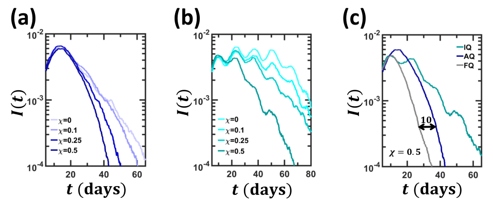

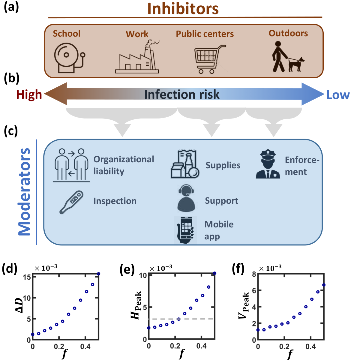
Fig. 4: The impact of Alternating quarantine. Full size.
![[Uncaptioned image]](2004.01453v4/x1.png)
References
- [1] R.M. Anderson, H. Heesterbeek, S. Klinkenberg and T.D. Hollingsworth. How will country-based mitigation measures influence the course of the COVID-19 epidemic? The Lancet, 395:10228, 2020.
- [2] Moritz U. G. Kraemer, Chia-Hung Yang, Bernardo Gutierrez, Chieh-Hsi Wu, Brennan Klein, David M. Pigott, , Louis du Plessis, Nuno R. Faria, Ruoran Li, William P. Hanage, John S. Brownstein, Maylis Layan, Alessandro Vespignani, Huaiyu Tian, Christopher Dye, Oliver G. Pybus, and Samuel V. Scarpino. The effect of human mobility and control measures on the covid-19 epidemic in china. Science, 2020.
- [3] Alex Arenas, Wesley Cota, Jesus Gomez-Gardenes, Sergio Gomez, Clara Granell, Joan T. Matamalas, David Soriano-Panos, and Benjamin Steinegger. Derivation of the effective reproduction number r for covid-19 in relation to mobility restrictions and confinement. medRxiv, 2020.
- [4] Benjamin Maier and Dirk Brockmann. Effective containment explains subexponential growth in recent confirmed covid-19 cases in china. Science, page eabb4557, 04 2020.
- [5] Bnaya Gross, Zhiguo Zheng, Shiyan Liu, Xiaoqi Chen, Alon Sela, Jianxin Li, Daqing Li, and Shlomo Havlin. Spatio-temporal propagation of covid-19 pandemics. medRxiv, 2020.
- [6] J. Hellewell et al. Feasibility of controlling COVID-19 outbreaks by isolation of cases and contacts. Lancet Global Health, 8:488, 2020.
- [7] Anatoly Zhigljavsky, Roger Whitaker, Ivan Fesenko, Yakov Kremnitzer, and Jack Noonan. Comparison of different exit scenarios from the lock-down for covid-19 epidemic in the uk and assessing uncertainty of the predictions. medRxiv, 2020.
- [8] Shen Chen Yaneer Bar-Yam. COVID-19: How to win, 2020.
- [9] J.M. Epstein. Modelling to contain pandemics. Nature, 460:687, 2009.
- [10] A. Hacohen, R. Cohen, S. Efroni, B. Barzel and I. Bachelet . Digitizable therapeutics for decentralized mitigation of global pandemics. Nature Scientific Reports, 9:14345, 2019.
- [11] Per Block, Marion Hoffman, Isabel J. Raabe, Jennifer Beam Dowd, Charles Rahal, Ridhi Kashyap, and Melinda C. Mills. Social network-based distancing strategies to flatten the covid 19 curve in a post-lockdown world, 2020.
- [12] Q. Li et al. Early transmission dynamics in Wuhan, China, of novel coronavirus-infected pneumonia. N Engl J. Med., 382:1199, 2020.
- [13] WHO. Coronavirus disease (COVID-2019) situation report 30. 2020.
- [14] Luca Ferretti, Chris Wymant, Michelle Kendall, Lele Zhao, Anel Nurtay, Lucie Abeler-Dörner, Michael Parker, David Bonsall, and Christophe Fraser. Quantifying sars-cov-2 transmission suggests epidemic control with digital contact tracing. Science, 2020.
- [15] NM Ferguson, D Laydon, G Nedjati-Gilani, N Imai, K Ainslie, M Baguelin, S Bhatia, A Boonyasiri, Z Cucunubá, G Cuomo-Dannenburg, et al. Impact of non-pharmaceutical interventions (npis) to reduce covid-19 mortality and healthcare demand. imperial college covid-19 response team, 2020.
- [16] Jantien A Backer, Don Klinkenberg, and Jacco Wallinga. Incubation period of 2019 novel coronavirus (2019-ncov) infections among travellers from wuhan, china, 20–28 january 2020. Eurosurveillance, 25, 2020.
- [17] Natalie M Linton, Tetsuro Kobayashi, Yichi Yang, Katsuma Hayashi, Andrei R Akhmetzhanov, Sung-mok Jung, Baoyin Yuan, Ryo Kinoshita, and Hiroshi Nishiura. Incubation period and other epidemiological characteristics of 2019 novel coronavirus infections with right truncation: a statistical analysis of publicly available case data. Journal of clinical medicine, 9, 2020.
- [18] Yang Tao, Panke Cheng, Wen Chen, Peng Wan, Yaokai Chen, Guodan Yuan, Junjie Chen, Da Huo, Ge Guan, Dayu Sun, et al. High incidence of asymptomatic sars-cov-2 infection, chongqing, china. 2020.
- [19] Kenji Mizumoto, Katsushi Kagaya, Alexander Zarebski, and Gerardo Chowell. Estimating the asymptomatic proportion of coronavirus disease 2019 (covid-19) cases on board the diamond princess cruise ship, yokohama, japan, 2020. Eurosurveillance, 25, 2020.
- [20] Xingfei Pan, Dexiong Chen, Yong Xia, Xinwei Wu, Tangsheng Li, Xueting Ou, Liyang Zhou, and Jing Liu. Asymptomatic cases in a family cluster with sars-cov-2 infection. The Lancet Infectious Diseases, 20, 2020.
- [21] Xiaoxia Lu, Liqiong Zhang, Hui Du, Jingjing Zhang, Yuan Y Li, Jingyu Qu, Wenxin Zhang, Youjie Wang, Shuangshuang Bao, Ying Li, et al. Sars-cov-2 infection in children. New England Journal of Medicine, 2020.
- [22] Jaffar A Al-Tawfiq. Asymptomatic coronavirus infection: Mers-cov and sars-cov-2 (covid-19). Travel medicine and infectious disease, 2020.
- [23] Philippe Colson et al. Children account for a small proportion of diagnoses of sars-cov-2 5 infection and do not exhibit greater viral loads than adults.
- [24] Huan Song, Jun Xiao, Jiajun Qiu, Jin Yin, Huazhen Yang, Rui Shi, and Wei Zhang. A considerable proportion of individuals with asymptomatic sars-cov-2 infection in tibetan population. medRxiv, 2020.
- [25] Yuanyuan Dong, Xi Mo, Yabin Hu, Xin Qi, Fan Jiang, Zhongyi Jiang, and Shilu Tong. Epidemiology of covid-19 among children in china. Pediatrics, 2020.
- [26] Guy P. Nason. Rapidly evaluating lockdown strategies using spectral analysis: the cycles behind new daily covid-19 cases and what happens after lockdown, 2020.
- [27] United Nations Department of Economic and Social Affairs. Household size and composition 2019. https://population.un.org/Household/index.html/countries/840.
- [28] Yinon M Bar-On, Avi Flamholz, Rob Phillips, and Ron Milo. Sars-cov-2 (covid-19) by the numbers. eLife, 9, 2020.
- [29] Qun Li, Xuhua Guan, Peng Wu, Xiaoye Wang, Lei Zhou, Yeqing Tong, Ruiqi Ren, Kathy SM Leung, Eric HY Lau, Jessica Y Wong, et al. Early transmission dynamics in wuhan, china, of novel coronavirus–infected pneumonia. New England Journal of Medicine, 2020.
- [30] Xuan Jiang, Simon Rayner, and Min-Hua Luo. Does sars-cov-2 has a longer incubation period than sars and mers? Journal of medical virology, 2020.
- [31] Stephen A Lauer, Kyra H Grantz, Qifang Bi, Forrest K Jones, Qulu Zheng, Hannah R Meredith, Andrew S Azman, Nicholas G Reich, and Justin Lessler. The incubation period of coronavirus disease 2019 (covid-19) from publicly reported confirmed cases: estimation and application. Annals of internal medicine, 2020.
- [32] S.A. Lauer et al. The incubation period of coronavirus disease 2019 (COVID-19) from publicly reported confirmed cases: estimation and application. Ann Intern Med., 172:577–582, 2020.
- [33] E. Dong, H. Du and L. Gardner. An interactive web-based dashboard to track COVID-19 in real time. The Lancet Infectios Diseases, 2020.
- [34] https://data.worldbank.org/indicator/sh.med.beds.zs.
- [35] Omer Karin, Yinon M. Bar-On, Tomer Milo, Itay Katzir, Avi Mayo, Yael Korem, Boaz Dudovich, Eran Yashiv, Amos J. Zehavi, Nadav Davidovich, Ron Milo, and Uri Alon. Adaptive cyclic exit strategies from lockdown to suppress covid-19 and allow economic activity. medRxiv, 2020.
- [36] S. Mallapaty. The coronavirus is most deadly if you are older and male - new data reveal the risks. Nature, page 16, 2020.
- [37] M. Bonafè et al. Inflamm-aging: why older men are the most susceptible to sars-cov-2 complicated outcomes. Cytokine Growth Factor Review, page 33, 2020.
- [38] Y. Xie et al. Epidemiologic, clinical, and laboratory findings of the covid-19 in the current pandemic: systematic review and meta-analysis. BMC Infect Dis., page 640, 2020.
- [39] Harshad Khadilkar, Tanuja Ganu, and Deva P Seetharam. Optimising lockdown policies for epidemic control using reinforcement learning, 2020.
- [40] Alex Tawse, Vanessa M Patrick, and Dusya Vera. Crossing the chasm: Leadership nudges to help transition from strategy formulation to strategy implementation. Business Horizons, 62, 2019.
- [41] Michael R Baumann and Bryan L Bonner. An Expectancy Theory Approach to Group Coordination: Expertise, Task Features, and Member Behavior. Journal of Behavioral Decision Making, 30, 2017.
- [42] V H Vroom. Work and Motivation. Wiley, New York NY, 1964.
- [43] Ata ul Musawir, Saipol Bari Abd-Karim, and Mohd Suhaimi Mohd-Danuri. Project governance and its role in enabling organizational strategy implementation: A systematic literature review. International Journal of Project Management, 38, 2020.
Alternating quarantine for
sustainable epidemic mitigation
Supplementary Information
I Modeling the spread
I.1 The unmitigated spread
I.1.1 Population network
We consider households , each including individuals, where is a random variable extracted from the household size distribution (Table 5). Together these households comprise the total population, in which the number of individuals is given by . Hence, the -th individual, resides together with her cohabitants at her household . Taking , and the average household size to be , we arrive at a total population of individuals.
To construct the social network , we consider two types of links: Within a household there are no barriers, hence the in-house connection network is simply a union of disjoint cliques representing . This results in isolated cliques whose size is distributed via . Out of home connections, , can be potentially drawn between any pair of nodes , capturing external social links, occurring at work, school or other public places. The external network can be admit any desired degree distribution via the configuration model framework [1]. In our simulations we used two archetypal constructions - the Erdős-Rényi (ER) random graph (main text), in which is bounded, and a scale-free (SF) network, where (Sec. II). In both cases we set the average degree to . The final network contains all links in and .
I.1.2 Temporality
The links in are not constantly active. Rather, they represent potential infectious interactions, switching between periods of activity, when infections can take place, and inactivity, when infections are barred. Throughout the daily cycle we have active during the day, 8:00 AM to 8:00 PM, and active during the after-hours, 8:00 PM to 8:00 AM the next day. This captures a typical routine, in which individuals interact sporadically, i.e. links are switched on and off, out of home in the day-time, and in-house at night.
Dividing each day into minute segments, , we generate a random sequence of temporal activity/inactivity instances for and . During the day, the probability for activation of each link in per interval is set to . Similarly, during the night we have probability for activation. The result is a stochastic pattern of potentially infectious interactions, in which the idling time between subsequent instances of activity follows a geometric distribution or for and , respectively. On average, we have links active
| (5) |
hours, and active for
| (6) |
hours, per daily cycle.
There are two exceptions to the above random activation rules:
- •
Isolation. In case node is known to be infected, i.e. symptomatic (Sec. I.3), then ’s entire household enters isolation. All nodes in remain at home until the household is cleared to retain its activity. Under these conditions only is activated with probability throughout the entire hour cycle, and links remain idle. Consequently, when in isolation, in-house interactions become more extensive, as they have more potential instances of infection, then during periods of normal activity.
- •
Collocation. For consistency, if at a certain instance, both links and are simultaneity active, then the triad link is also activated. Indeed, a concurrent collocation of and , implies, by transitivity, an inevitable collocation also of . This alllows us to capture potential correlations in the temporal patterns of the interactions.
A summary of all temporal network parameters appears in Table 1.
| Parameter | Description | Value |
|---|---|---|
| Population size | ||
| Number of households | ||
| degree distribution | Erdős-Rényi or scale-free | |
| Household size distribution | Empirically obtained, Table 5 | |
| Average degree | ||
| Average household size | ||
| Probability of link activation | Varied | |
| Probability of link activation | Varied | |
| Mean daily infection time via | Eq. (5) | |
| Mean daily infection time via | Eq. (6) | |
| Fraction of in-house infections | Extracted from data/simulation | |
| infection growth rate | Extracted from data/simulation |
I.2 Mitigation
During mitigation, the quarantined households express only throughout the hour cycle, with all their links rendered inactive. If a household member is defective, their links continue to activate as usual. Partitioning the population, as in AQ or HQ, for example, is done at household level - namely households are randomly split among the cohorts. In each realization, we instigate the mitigation at a time when the fraction of infections exceeds a significant threshold. We set this threshold at
| (7) |
namely the time point where the total infected population is of the order of .
I.3 Disease dynamics
We begin with a fully susceptible () population, and introduce a small fraction of exposed () individuals. The potential transitions that ensue are shown in Fig. 9, whose main transitions include:
- •
Infection. At any encounter between a susceptible node and a pre-symptomatic or infected node , may become exposed. By encounter we relate to an instance in which the link in or is active. The probability of infection at each encounter depends on the nature of the link, set to for links and for . External interactions , between associates, are typically less physical than in-house interactions between e.g., family members, hence, typically . In practice, however, we can incorporate these probabilities into the encounter probabilities themselves, . Indeed, stating that and interact with probability and then infect with probability , is equivalent to setting their interaction probability to , and having infections occurring with certainty. Hence, for simplicity we set , and encapsulate the infection probabilities within the parameters in (5) and (6).
- •
Infection classification. During the simulation of the spread we keep count of the type of each infection. Infections occurring via links add to the in-house infection count ; infections occurring out of home, through contribute to .
- •
Infection cycle. Once a node becomes exposed it begins to transition between states according to Fig. 9a. Exposed nodes have contracted the virus, but are not yet infectious. These nodes are randomly split between with probability and with probability . This decides whether these nodes are pre-symptomatic, and eventually will develop symptoms, or asymptomatic, reaching recovery without even experiencing symptoms. The remaining disease cycle continues according to the illustration. For example, nodes in will later transition to one of the infected stated or with probabilities and , respectively; the remaining are accounted for in the trajectory. Similarly, nodes, after some time enter the hospitalized state , after which the recover with probability , and decease with probability .
Note that ventilated individuals are, by definition, also hospitalized. However, in out implementation we consider these as two isolated groups, i.e. ventilated vs. hospitalized without ventilation. Therefore, at all times we have , comprising the entire population. Presenting our results we used the normalized compartments , which satisfy
(8) - •
Transition times. The amount of time a node remains at a state (other than ) is chosen at random according to probability density . We identify specific processes for which variability in the transition time may impact the effectiveness of alternating quarantine (AQ). For example, the time from exposure to infectiousness, or the time for asymptomatic individuals to recover are crucial. Deviations from the mean in these transition times may interfere with AQ’s disease cycle synchronization. For instance, if a node remains asymptomatic for, e.g., weeks, which is beyond the average time to recovery, its infectiousness may spillover between AQ’s subsequent activity cycles, allowing it to resume activity while still infectious. Similarly, if the pre-symptomatic stage is extended significantly beyond the day average, an infected individual in week may not yet develop symptoms during their isolation at week , once again, reducing the efficiency of AQ in removing invisible spreaders. Therefore, for these highly relevant transitions we placed a special emphasis to avoid underestimating their potential time-scale heterogeneity. In particular we identified four relevant processes: , the time until an exposed asymptomatic individual () becomes infectious (); , the time until an asymptomatic infectious node recovers; , the time until an exposed pre-symptomatic individual () becomes infectious () and , the time for an infectious pre-symptomatic () to show symptoms ( or ). For these four functions we used a Weibull distribution, as explained in Sec. IV.1. This distribution allows us to capture the potentially variable time-scales across the population, thus testing AQ under realistically challenging conditions.

I.4 Evaluating and
Our model parameters control the spreading dynamics via the temporal probabilities and , and their subsequent and in (5) and (6), that govern the rate of infections in and out of home. Once these parameters are set, the simulating results of the unmitigated spread allow us to evaluate the infection growth rate and the in-house transmission rate :
- •
In-house infection rate . During the simulation we keep count of the source of all infections. Infections occurring via , amounting to are external, while those that transmit along links, , are internal. The parameter captures the percentage of transmissions that occurred in-house as
(9) - •
The infection growth rate . To evaluate we observe the overall infected population vs at the early stages of the spread, and fit it to an exponential of the form
(10) Obtaining the slope of the resulting growth on semi-logarithmic axes we extract from the simulation results. Note that depends on the slope, not on the pre-factor, hence it is insensitive to the size of the initial outbreak, or to the fraction of cases detected via testing, providing a fair comparison between different realizations or empirical datasets.
A crucial point is to select the range in from which to extract the slope. Indeed, for very small , due to the stochastic nature of our simulations, is still small, and still discrete. In this limit, the observed results are subject to high levels of noise and may not yet exhibit a clear exponential behavior. On the other hand if is too large, we approach the peak of , where the exponential approximation fails again, this time due to the accumulation of herd immunity. Therefore, to be consistent across all our simulations we evaluated from the time window
(11) where is the time of peak infection. Evaluating from empirical data is explained in Sec. IV.
Note, that and are not the model parameters. Rather they emerge from the stochastic simulation results, after setting the model parameters and . Therefore, we do not have direct control over these parameters, as seen in, e.g., Fig. 4 of the main text, where were only approximately equal across the different panels. Roughly speaking, we can link these parameters to each other. A large , for example enhances transmission, and hence increases . The parameter , on the other hand, grows as is increased and is decreased, capturing a state in which in-house transmissions are more prevalent than external ones.
II Results obtained under a scale-free
Our strategy in testing AQ is to examine it systematically under varying relevant scenarios. Specifically, for unknown parameters, such as and , we simulated an array of different setting, scanning the space of potential values (e.g., Fig. 4 of main text). Other unknown factors relate to the structural characteristics of the external network . Most importantly, in the context of epidemic spreading - its degree distribution, which has been shown to significantly impact the patterns of spread [2]. To eliminate this potentially confounding factor we now re-examine AQ, repeating our simulations, this time extracting from the scale-free network ensemble (). We find, in Figs. 10 and 11 that AQ continues to provide the optimal mitigation also under these conditions.


III Alternating quarantine under selective isolation

In the main take we used a typical disease cycle, capturing the average individual’s response to SARS-CoV-2. We now consider two parallel cycles, one for healthy individuals and the other for the vulnerable, such as people with background diseases or the elderly. The two cycles differ mainly in their transition probabilities. For example, while only of the healthy individuals develop critical symptoms (), among the vulnerable population the number is set to . The complete disease cycle for the Typical, Healthy and Vulnerable population [3, 4, 5] appears in Table 2.
To track the spread in the presence of healthy/vulnerable populations we repeated the simulation described in Sec. I, this time splitting the population into healthy and vulnerable nodes [6]. We track three indicators that help us assess the performance of all strategies (Fig. 12): Hospitalization rate , ventilation rate and mortality . As expected, AQ (Fig. 12)a,d,g, light blue) continues to outperform IQ (light turquoise) and HQ (light red) also under this variable disease cycle.
Next, we added an additional component of selective isolation, in which the vulnerable nodes () remain under constant quarantine. For example, in AQ this implies that the weekly alternations are limited only to the healthy . Under these conditions the vulnerable individuals cannot be infected via external links . They can still, however, experience secondary infection through , in case one of their healthy cohabitants contracted the virus. As expected, such selective isolation enhances the performance of all the strategies, lowering hospitalization, ventilation and mortality (Fig. 12b,e,h). This improvement, we emphasize, is not unique to AQ, making it clear that selective isolation is a desirable component within any mitigation strategy. In Fig. 12c,f,i we present our three performance measures, , and with (dark) and without (light) selective isolation, further indicating the importance of protecting the vulnerable population.
| Probability | Typical | Healthy | Vulnerable |
|---|---|---|---|
| 0.3 | 0.32 | 0.25 | |
| 0.55 | 0.56 | 0.45 | |
| 0.1 | 0.08 | 0.2 | |
| 0.05 | 0.04 | 0.1 | |
| 0.85 | 0.86 | 0.79 | |
| 0.15 | 0.14 | 0.21 | |
| 0.5 | 0.5 | 0.5 | |
| 0.5 | 0.5 | 0.5 |
IV Data analysis and parameter selection
IV.1 Constructing the distributions
Most of the parameters described in Section I were chosen based on observed values of the characteristic SARS-CoV-2 infection cycle. For the density functions , we have used a Weibull or a Geometric distribution, the former - inspired both by other infections of the Corona variety [7], as well as recent inidcations pretainig to SARS-CoV-2 [8, 9, 10]. The Weibull distribution allows for potentially high variability across the population, providing a challenging testing ground for AQ.
To estimate the parameters of the Weibull distributions we collected data on the average and median of the relevant transition times [8, 7]. This allowed us to infer the Weibull parameters and via
As median values were available only for and , we first calculated the parameter for these transitions, obtaining, for both . This is not surprising as , the shape parameter, controls the type of the Weibull distribution, which is expected to be similar for processes driven by similar mechanisms. This is as opposed to , the location parameter, which is not intrinsic to the shape of the distribution, but rather shifts right or left as the mean is changed. Hence, it is expected that is uniform for the different transition-time distributions, while may change according to their mean. With this in mind, we estimated for the other two distributions, and , where the median was inaccessible from data. See Table 3 for the different values of mean, and median we have used, and the inferred and .
| Duration | Distribution | Observations | Parameters | ||
|---|---|---|---|---|---|
| Mean | Median | ||||
| Weibull | 4 | 4.42 | |||
| Weibull | 10 | 8.6 | 11.04 | 1.47 | |
| Weibull | 2 | 2.21 | |||
| Weibull | 5 | 4.3 | 5.52 | 1.47 | |
| Mean | |||||
| Geometric | 5 | 0.2 | |||
| Geometric | 4 | 0.25 | |||
| Geometric | 3 | 0.333 | |||
| Geometric | 11 | 0.091 | |||
| Geometric | 13 | 0.077 | |||
IV.2 Estimating the infection growth
As defined above, the parameter represents the exponential growth rate of the known infectious nodes . This parameter is difficult to predict directly from the knwon disease time-scales, especially as the infection rate is hidden, hence we must infer it from observation. Moreover, as the disease progresses, precautions like social distancing and wearing masks affect both the rate of interaction and the probability of infection, leading to change over time. Therefore, to asses for the unmitigated spread, we have focus on the period before such measures were taken.
We collected data on the number of confirmed cases in countries. These countries have been selected for their prominent number of casesm and to obtain a balanced representation between southern and northern hemisphere destinations. The data set was compiled by and obtained from the Johns Hopkins University Center for Systems Science and Engineering (JHU CSSE) on April 11th 2020 and is available online here: https://data.humdata.org/dataset/novel-coronavirus-2019-ncov-cases [11].
To capture the relevant time-window for the exponential growth approximation we used data-points starting days before lock-down and ending days after it. Indeed, earlier than this point, cases may be underestimated by a yet unprepared system, and beyond this window, the lock-down may begin affecting the observed slope. As clearly seen in Fig. 3 of the main text, within this time-window the spread can be well-approximated by an exponential growth of the form (10). To extract the slope we used linear regression on , yielding the estimator for the growth rate in each country, as detailed in Table 4 and in Fig. 13. We find that estimators are narrowly distributed around an average of , the value we used as our default, i.e. unmitigated spreading parameter.

| Country | Population | First case | Lock-down | |
|---|---|---|---|---|
| Italy | 60 | 10 | 38 | 0.32 |
| USA | 328 | 3 | 61 | 0.3 |
| Spain | 47 | 19 | 43 | 0.34 |
| Israel | 9 | 36 | 54 | 0.19 |
| Germany | 83 | 7 | 52 | 0.26 |
| Norway | 5.4 | 38 | 49 | 0.32 |
| Colombia | 52 | 49 | 56 | 0.28 |
| Argentina | 45 | 45 | 50 | 0.22 |
| Netherlands | 17 | 39 | 54 | 0.21 |
| N. S. Wales | 8 | 5 | 52 | 0.18 |
| Austria | 9 | 35 | 45 | 0.3 |
| UK | 56 | 10 | 46 | 0.29 |
IV.3 Estimating the household size distribution
We used a United Nations database [12] to collect data on the distribution of household sizes across different countries. The data, summarized in Table 5, was compiled by and obtained from the United Nations, Department of Economic and Social Affairs, Population division.
| Country | 1 | 2-3 | 4-5 | 6 | Average |
|---|---|---|---|---|---|
| Italy | 0.31 | 0.47 | 0.21 | 0.01 | 2.4 |
| Germany | 0.39 | 0.47 | 0.13 | 0.01 | 2.05 |
| USA | 0.28 | 0.49 | 0.19 | 0.04 | 2.5 |
| Israel | 0.21 | 0.4 | 0.28 | 0.11 | 3.14 |
| Spain | 0.19 | 0.53 | 0.26 | 0.02 | 2.69 |
| Norway | 0.4 | 0.41 | 0.18 | 0.01 | 2.22 |
| Model | 0.3 | 0.46 | 0.2 | 0.04 | 2.6 |
References
- [1] M.E.J. Newman. Networks - an introduction. Oxford University Press, New York, 2010.
- [2] R. Pastor-Satorras, C. Castellano, P. Van Mieghem and A. Vespignani. Epidemic processes in complex networks. Rev. Mod. Phys., 87:925–958, 2015.
- [3] S. Mallapaty. The coronavirus is most deadly if you are older and male - new data reveal the risks. Nature, page 16, 2020.
- [4] M. Bonafè et al. Inflamm-aging: why older men are the most susceptible to sars-cov-2 complicated outcomes. Cytokine Growth Factor Review, page 33, 2020.
- [5] Y. Xie et al. Epidemiologic, clinical, and laboratory findings of the covid-19 in the current pandemic: systematic review and meta-analysis. BMC Infect Dis., page 640, 2020.
- [6] United Nations report. World population ageing 2019.
- [7] Yinon M Bar-On, Avi Flamholz, Rob Phillips, and Ron Milo. Sars-cov-2 (covid-19) by the numbers. eLife, 9, 2020.
- [8] Natalie M Linton, Tetsuro Kobayashi, Yichi Yang, Katsuma Hayashi, Andrei R Akhmetzhanov, Sung-mok Jung, Baoyin Yuan, Ryo Kinoshita, and Hiroshi Nishiura. Incubation period and other epidemiological characteristics of 2019 novel coronavirus infections with right truncation: a statistical analysis of publicly available case data. Journal of clinical medicine, 9, 2020.
- [9] S.A. Lauer et al. The incubation period of coronavirus disease 2019 (COVID-19) from publicly reported confirmed cases: estimation and application. Ann Intern Med., 172:577–582, 2020.
- [10] Jantien A Backer, Don Klinkenberg, and Jacco Wallinga. Incubation period of 2019 novel coronavirus (2019-ncov) infections among travellers from wuhan, china, 20–28 january 2020. Eurosurveillance, 25, 2020.
- [11] E. Dong, H. Du and L. Gardner. An interactive web-based dashboard to track COVID-19 in real time. The Lancet Infectios Diseases, 2020.
- [12] United Nations Department of Economic and Social Affairs. Household size and composition 2019. https://population.un.org/Household/index.html/countries/840.