Randomized Kernel Multi-view Discriminant Analysis
Abstract
In many artificial intelligence and computer vision systems, the same object can be observed at distinct viewpoints or by diverse sensors, which raises the challenges for recognizing objects from different, even heterogeneous views. Multi-view discriminant analysis (MvDA) is an effective multi-view subspace learning method, which finds a discriminant common subspace by jointly learning multiple view-specific linear projections for object recognition from multiple views, in a non-pairwise way. In this paper, we propose the kernel version of multi-view discriminant analysis, called kernel multi-view discriminant analysis (KMvDA). To overcome the well-known computational bottleneck of kernel methods, we also study the performance of using random Fourier features (RFF) to approximate Gaussian kernels in KMvDA, for large scale learning. Theoretical analysis on stability of this approximation is developed. We also conduct experiments on several popular multi-view datasets to illustrate the effectiveness of our proposed strategy.
1 Introduction
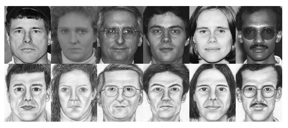
Multi-view learning [23, 42, 48, 18] or learning with multiple different feature sets is rapidly growing research area with practical success in important applications. For example, a person can be described by visual light face image, sketch, near infrared face image, iris, fingerprint, palmprint or signature with information secured from many different sources (e.g., distinct angles). Our task is to classify an object from one view, given the information from other views. For instance, Figure 1 shows some samples from two different views in the CUFSF multi-view dataset (more detailed dataset description is provided in the experiments section). Here, each person represents a object class, and we would like to classify a sketch given all the label information of the photos, or vise versa. In many cases, the views can be quite different as well. An example is the content-based web-image retrieval, where an object can be identified by the text depicting the image or visual features from the image itself. Here the text and image can be regarded as two distinct views, of the same object.
In this paper, we focus on multi-view subspace learning, which aims to learn a common subspace shared by all different views. The research on multi-view learning started with “two-view” learning. The canonical correlation analysis (CCA) [20, 19, 49] is perhaps the most well-known two-view unsupervised algorithm. CCA finds the linear projections for two views respectively which have maximum correlation with each other. The discriminative variants of CCA were studied in [32, 40]. The paper [30] provided common discriminant feature extraction to maximize the inter-class separability and meanwhile minimize the intra-class scatter. Multi-view CCA (MCCA) [33, 35] was proposed to secure one common subspace for all views, under unsupervised setting. Generalized multi-view analysis (GMA) framework [36] took advantage of class information, resulting in a discriminant common space. The authors of [37] presented the multi-model discriminant analysis (MMDA) to decompose variations in a dataset into independent modes (factors). The multi-view discriminant analysis (MvDA) was proposed by [23], which learned projections for different views jointly via Fisher discriminant analysis. In [7], the authors proposed a variant called MvMDA, which differs from standard MvDA in the definition of inter-class and intra-class covariance matrices.
In many cases, non-linear kernel has stronger learning capacity than linear kernel. Hence, to enhance performance of standard MvDA algorithm, in this paper we seek to kernelize multi-view discriminant analysis, and derive so-called kernel MvDA (KMvDA). However, it is known that a direct implementation of nonlinear kernels is difficult for large-scale datasets, since even for a medium-sized dataset with only 100,000 instances, the 100,000100,000 kernel matrix has entries, which is essentially not feasible for most machines that people use daily. Therefore, in practical applications, being capable of linearizing nonlinear kernels is highly welcome [4, 27, 26]. Random Fourier features (RFF’s) [34, 24] is a celebrated algorithm to linearly approximate Gaussian (RBF) kernel, which has been widely used and studied in literature [31, 41] on clustering, CCA, PCA, classification, etc. For two data points, the inner product of linearized Fourier features is unbiased estimator of the true RBF kernel. By using faster linearized algorithms, we are able to exploit the learning power of non-linear kernel (e.g., RBF kernel) in linear time when dealing with large-scale datasets.
Our contributions. In this paper, we first derive a kernelized MvDA, and then apply random Fourier features to KMvDA and demonstrate its feasibility for large scale learning. To the best of our knowledge, this is the first attempt in literature to randomize multi-view discriminant learning. It is shown that by approximation, the change in eigenspace (and hence the projections) could be bounded and converges to zero as we increase the number of random features. Experimental results provide evidence on the advantage of KMvDA, as well as the effectiveness of the linearized approximation.
Roadmap. In Section 2, we introduce some preliminaries on multi-view discriminant analysis (MvDA) and eigenspace comparison. In Section 3, we formulate the kernel MvDA (KMvDA). In Section 4, we introduce the kernel approximation scheme and provide theoretical analysis of the approximation error on the subspace learned by KMvDA. In Section 5, we conduct experiments to show the effectiveness of our method. In the last section, we discuss some relevant topics and conclude the paper.
2 Preliminaries
2.1 Problem setting and notations
In this paper, we denote a multi-view dataset by with the instances where is the -th instance from the -th class of the -th view of dimension, denotes the number of classes, is the number of views. represents the instances from the -th view. denotes the number of instances from the -th class of the -th view, and is the number of observations from the -th class of all views. Let denote the total number of examples from all views. Let denote the class label of . Let denote the view-specific linear projections that we aim to learn. Throughout the paper, denotes matrix Frobenius norm and is the operator norm for matrix and Euclidean norm for vector.

2.2 Multi-view discriminant analysis
Multi-view discriminant analysis (MvDA) [23] aims to find view-specific linear projections which can respectively transform the instances from views to one discriminant common space, by minimizing the within-class variation and maximizing the between-class variation. Instances from views are then projected onto the same common space by . Figure 2 depicts the idea and framework of MvDA. To achieve cross-view discrimination, the within-class variation from all views should be minimized while the between-class variation from all views should be maximized in the common space.
More specifically, MvDA is a generalization of linear discriminant analysis (LDA) [19] for multi-view learning. They share the same type of objective function (i.e., the Rayleigh quotient),
| (1) |
where , .
The terms and can be seen as the within-class scatter matrix and between-class scatter matrix for multi-view learning, respectively. The -th column and the -th row block matrix of , which is denoted by , is defined as:
The term is the -th column and the -th row block matrix of and defined as
with .
Basically, MvDA extends LDA to multi-view setting with carefully designed block covariance matrices that aim to achieve accurate multi-view classification. The standard approach for solving the optimization problem (1) is by transforming it into a generalized eigenvalue problem, which will be introduced in the next sub-section.
2.3 Eigenspace Comparison
A standard eigenvalue problem (SEP), given a square matrix A, is to solve for vector and scalar . Feasible ’s are called the eigenvalues (or spectrums), and ’s are called eigenvectors. For SEP, there exist many well-known results on the eigenvalues (e.g., Weyl’s theorem) when a small perturbation is added to . The Davis-Kahan theorem (e.g., the theorem) provides bounds on the change of angles between eigenvectors, which could be regarded as a measure of the change of eigenspace. These theorems cast additional restrictions on the eigenvalues by assuming the existence of eigengaps.
A generalized eigenvalue problem (GEP), given , is to find the solution to the system
| (5) |
and each pair of and that satisfies this equation is called a pair of generalized eigenvalue and generalized eigenvector. One natural idea to study the perturbation of generalized eigen system (5) is to left-multiply the inverse of on both sides and yields an ordinary eigenvalue problem , provided that is invertible. However, when is singular, this approach would fail but feasible solution to GEP may still exists [38, 39, 9]. More specifically, when matrices and have common null space, the set of eigenvalues may become the whole complex plane. In this case, the problem is said to be ill-disposed since the spectrum is extremely unstable. The Crawford number, defined as
| (6) |
is very important in this context. Here means the conjugate transpose. For real matrices, we could also write it as . Matrix pair is said to be definite if holds. In this case, the problem is called a definite problem. This technical condition ensures that and not having interlacing null space.
It is shown in [38] that without special information, the eigenvectors may be very sensitive to small perturbations, but the subspace spanned by them may be stable. In the following, we summarize some related concepts and results on subspace perturbation. Notations with tildes denote the counterparts in perturbed problem.
Definition 1.
Suppose is a definite matrix pair. A subspace is an eigenspace of if
For a definite pair, there always exists with , , such that
| (7) |
where , and , and a similar decomposition holds for perturbed matrices. Clearly, is an eigenspace for . Let be the column space of . Analyzing a rotation between and shows that
| (8) |
represents the canonical angles between some sets of suitably chosen base vectors of and . Hence, becomes a good measure of the difference between these two subspaces. The following theorem depicts the relationship between , the gap between subspaces and corresponding projection operators.
Theorem 1.
This equivalence makes a commonly used measure for the difference between two subspaces. We also define the chordal distance between points , as
| (9) |
which is crucial for comparing eigenvalues in generalized eigen problems. It is invariant under rotation about the origin and can handle large, or infinite eigenvalues by measuring the distances on the Riemann sphere.
3 Kernel Multi-view Discriminant Analysis
For many linear learners, kernel trick enables us to access a much higher, possibly infinite dimensional feature space by operating in an inner product space associated with a proper Reproducing Kernel Hilbert Space (RKHS) [1]. Examples of kernel methods include kernel PCA, kernel SVM, etc. In this section, we combine kernel trick with MvDA and derive kernel MvDA (KMvDA).
3.1 KMvDA
Formulation. Without loss of generality, we look at one projection direction (e.g., the top eigenvector). Based on previous definitions, we rewrite and in matrix form:
| (10) |
| (11) |
where is a vector with all elements equal to one and the dimensionality of is the same as the number of the examples of the -th view; is a vector whose dimensionality is the same as that of and with the -th class equal to one and zero otherwise. In the rest of this section, the same computation is described in another inner product space , which is associated with the input space by map and a kernel function in a reproducing kernel Hilbert space (RKHS) such that for ,
Note that the feature space could have an arbitrarily large, possibly infinite dimensionality. However, explicit representation of the function is unnecessary as long as is a proper inner product space. By this mapping, the objective function of KMvDA becomes
where are projection directions of distinct views. By the well-known Representer Theorem in RKHS, there exists such that Therefore, we can re-write the objective function using the inner products in the feature space ,
| (15) |
where and are block matrices with entries , respectively, and is a block diagonal matrix. After some standard derivation, (3.1) eventually turns into solving the GEP
| (16) |
As the eigenvalues are invariant of scale, we denote in this paper that all eigenvalues for MvDA (and KMvDA) are of the form , along with the paired eigenvectors , . Note that, every is an -dimensional vector (recall that is the total number of samples). The -th projection direction of the -th view, , is set to be the slice at corresponding positions of the -th view. For our task, we choose projection directions as the eigenvectors associated with the largest eigenvalues. More precisely, we sort and project onto an -dimensional space with respect to .
Testing phase. Given a new test set , for a test example , we compute projections of the -th view in the kernel space by
where is the -th view of and represents the element-wise kernel function. If our goal is to classify based on view , we assign with the label of nearest neighbor of in the projected space, .
3.2 Kernels
In this paper, we focus on comparing two kernels. The linear kernel is simply defined as the inner product between two data points, which will serve as the baseline. For non-linear kernels, we consider the radial basis functions (RBF) kernel (i.e., the Gaussian kernel), which is the most commonly used kernel in statistical learning and many related fields [19]. The RBF kernel between two examples and is computed as
where is the kernel width hyper-parameter. It is well-known that the RBF kernel is shift-invariant and positive definite.
4 KMvDA with Randomized Kernels
As discussed precedingly, in many practical tasks, computing kernels is very expensive when the data size is large. Therefore, linearized kernels are important in many cases, as one can enjoy the benefits of kernel methods with a linear learner. In this section, we consider linearizing the RBF kernel in the KMvDA approach, which aims at approximating the learning performance of using exact RBF kernel, but in linear time complexity. The tool we use is the random Fourier features (RFF’s) [34, 24].
4.1 Random Fourier Features (RFF)
Given a shift-invariant kernel , let be its Fourier transformation. Since the measure and kernel are both real, we have
Here, Bochner’s theorem reveals that is a valid non-negative measure if the kernel is continuous positive definite, and hence we can express the kernel as an expectation. Therefore, one can use Monte-Carlo method to estimate the kernel by repeatedly sampling from . The features generated in this way are called random Fourier features (RFF’s). For the RBF kernel, based on trigonometric identities, one popular scheme is
where and . This construction achieves unbiasedness, i.e., . Let , we estimate the RBF kernel matrix by the mean of samples
| (17) |
and define estimates of matrices and as and using accordingly. Then we solve the problem to approximate the solution using exact kernel matrices.
Note that it has been shown in [24] that one can substantially improve the performance of RFF by normalizing the random features.
Obviously, RFF is tightly related to the method of random projections, which has become a popular technique to reduce data dimensionality while preserving distances between data points, as guaranteed by the celebrated Johnson-Lindenstrauss (J-L) Lemma and variants [22, 13]. There is a rich literature of research on the theory and applications of random projections, such as clustering, classification, near neighbor search, bio-informatics, compressed sensing, quantization, etc. [21, 11, 3, 5, 8, 15, 16, 43, 25, 14, 6, 17, 12, 45, 10, 28, 29].
4.2 Analysis of Randomized KMvDA
In this section, we investigate the subspace perturbation of using linearized RFF kernels, which directly determines the approximation efficiency of randomized KMvDA. In this sequel, notations with hats are defined for objects using approximated kernels. Without loss of generality, we assume that the number of examples in each view is the same, i.e., . Moreover, in each view, the number of observations per class is also the same (all equal to ). Besides, the classes are ordered in the same way in all views.
Lemma 1.
Proof.
First we can show that for , , where is a block matrix with diagonal matrices all equal to . The matrix contains exactly one non-zero eigenvalue, which equals to . Also, has positive eigenvalues equal to . Hence, we have , and all non-zero eigenvalues are equal to . By the definition of spectral norm is the largest magnitude of the eigenvalues, we obtain
Similar analysis could be applied to . According to fundamental linear algebra theories on block matrices, , with eigenvalues equal to and the rest eigenvalues being 1. In addition, , and all eigenvalues equal . Consequently, we obtain
Spectrum of large matrices. is a block matrix with repeating blocks . Hence, it admits the form of Kronecker product,
Consequently, the spectrum of consist of eigenvalues equal to , and the rest all equal to 0. Therefore, is positive semi-definite ( ). Recall the notation , we have
since for , . Define for as the off-diagonal block matrix of . We have
The eigenvalues of , by previous analysis, are -1 with multiplicity and 0 with multiplicity . By adding diagonal block matrix of identities, has eigenvalues of 0 and all others equal to 1. Therefore, is also positive semi-definite. ∎
Lemma 1 summarizes the spectral property of covariance structure sub-matrices. In particular, it illustrates that the generalized eigen problem arise from KMvDA is definite, and thus the following analysis would be valid.
4.2.1 A general perturbation bound
As discussed in preliminaries, a feasible solution to (16) exists as long as the GEP is definite, which does not require to be invertible. We first consider this general situation. The next lemma is a modified version of Theorem 3 in [31], which characterizes the kernel approximation error.
Lemma 2.
Suppose . Define linear approximation using random samples as (11). Then with probability ,
Proof.
We denote , and define random matrices . By the unbiasedness of RFF’s, we know that . To bound , we have , due to triangle inequality and boundedness of . In addition, we have
The second line is due to the fact that . Thus,
Applying matrix Bernstein inequality (Theorem 5.4.1 in [44]),
Now taking the right-had-side to be equal to , we derive a quadratic equation of . Solving for this equation gives us the desired bound. ∎
It is worth mentioning that because of the correlated entries of , in general this bound cannot be reduced in the absence of more structural assumptions. Now we are ready to study the eigenspace perturbation caused by kernel approximation.
Theorem 2.
For the GEP associated with KMvDA (i.e., (16)), assume that , , and admit decompositions (7) in the form of correspondingly. Let denote the set of eigenvalues of (16)). Assume the Crawford number , , and there are satisfying , and a real number , such that
| (18) | ||||
Denote , . Then the following inequality holds with probability ,
where
with for and . Also, we have
where is the number of random features.
Proof.
By Theorem 2, with probability , we have for ,
Denote this event . In this event, we have
where we recall that and . The last line holds because and , are both diagonal block matrix. Therefore,
It is easy to check that analogously using same argument. Moreover, by sub-multiplicity of operator norms, we have
since . Because is orthogonal, we have
and same inequality holds for . Hence we have
Putting all parts together and using Theorem 2.1 from [39], we get the desired bound. ∎
Condition (18) characterizes the separation of the generalized eigenvalues, where the eigengap can be interpreted in terms of chordal distance, defined by (9). Since the generalized eigenvalues are invariant of scale, we may force them on a unit semicircle in the upper plane. Note that in our problem, the generalized eigenvalues are in the form . Hence, we can scale each eigenvalue to . For any two pairs, we have
That is, the chordal distance between two eigenvalue pairs is the sine between the two rays with slopes and extended from the origin. Now we can translate (18) into angles (defined anti-clockwise): there exist a real number , , and , such that
Define as the gap between eigenvalue sets and . It is easy to check that , and
which implies that two sets of eigenvalues are well separated.
4.2.2 Perturbation of regularized problem
In practice, a regularization term is often added to GEP to handle singularity and make the system more stable and theoretically justifiable. Consider the following regularized GEP,
| (19) |
with a small constant. The problem is guaranteed to be definite, since , by Lemma 1, now becomes positive definite. More importantly, the invertibility of allows us to transform (19) into an SEP.
Theorem 3.
Let denote eigenvalues of , and be the eigenvalues of . Assume , then with probability ,
where . and are defined in Theorem 2.
Proof.
(of Theorem 3) Since is invertible, we may consider the SEP . We have
where . Here is induced by Theorem 4.1 in [47]. Since is positive definite and symmetric, is also symmetric and positive definite. Given that is symmetric and positive semi-definite, we know that is similar to a symmetric PSD matrix,
Hence, the eigenvalues of are all real and non-negative. Therefore, the eigenvalues is equivalent to singular values. The proof is then complete using the classic sin Theorem from [46]. ∎
From Theorem 2 and Theorem 3, we know that for both the original and regularized GEP, adopting linearized kernels could approximate the eigenspace of using exact kernel matrices, with a sufficiently large number of random features. This provides a theoretical support for the usage of RFF’s in KMvDA.
4.2.3 Comparison to Randomized CCA
In [31], the authors propose randomized CCA (RCCA), which also solves a GEP in the form of . However, it turns out that the problem is very different. More specifically,
- •
RCCA only involves two views, while KMvDA may include multiple views.
- •
The covariance matrices in RCCA is much simpler (block diagonal and linear in ), while for KMvDA the formulation is more sophisticated and quadratic in .
- •
We consider both the regularized problem and the general case of definite eigen problem without regularization, while [31] only studies the formulation with regularization.
5 Experiments
In this section, we present empirical results that illustrate the performance of KMvDA and linearized KMvDA using random Fourier features. The major goal is to show 1) KMvDA improves linear MvDA, and 2) randomized KMvDA is able to well approximate the performance of KMvDA with sufficient number of RFF’s.
5.1 Datasets
We test our algorithms on 3 popular datasets for multi-view learning research and applications. All datasets are publicly available.
Heterogeneous Face Biometrics (HFB) database has 100 persons in total, with 4 composed of visual (VIS) and 4 near infrared (NIR) face images for each person. This gives us a 2-view classification problem. For each view, we have 400 examples in total from 100 different people. We use the first 65 persons for training and the remaining 35 persons for testing. Each example is a image, which is transformed into 1024 features.
CUHK Face Sketch FERET (CUFSF) database is designed for research on face sketch synthesis and face sketch recognition. It includes 1194 persons (i.e., categories) from the FERET database. An example is given in Figure 1. This dataset contains two views: 1) face photo with lighting variation, and 2) sketch with shape exaggeration drawn by an artist when viewing this photo, both with dimensionality 5120. We use the first 650 examples as training set and the rest 544 examples for testing.
We use Multi-PIE dataset to test the performance of KMvDA on dealing with multiple views and larger sample size. The whole dataset contains more than 750,000 face images of 337 people, under different poses and from distinct views. In our experiment, we choose 7 different views (left , , , frontal, right , , ), three facial expressions (smile, neutral, disgust), and no flush illumination as the evaluation data. Each example is a 5,120 dimensional vector. This subset is divided into two parts: the images from the first 248 subjects with 4 randomly selected images under each pose of each person are utilized as training data and the images from the rest are utilized as test data.
5.2 Parameters and Performance Evaluation
Kernels. There is no tuning parameter for linear kernel. For RBF kernel, we fine-tune the parameter over a fine grid in the range of . The number of random Fourier features are chosen to be for each view. We set for RFF’s the same as fine tuned parameter value for RBF kernel to compare the approximation effectiveness of linearized methods. RFF vectors are normalized to have unit norm.
Evaluation. We mainly use the classification test accuracy to evaluate the model performance. We denote “-” when using training examples from view to classify test examples from view . The metric we use is the rank-1 recognition rate, which is the highest test accuracy among all parameter and projection dimensionality .
| Linear | RBF | RFF | ||
| HFB | NIR-VIS | 56.4 | 59.3 | 60.7 |
| VIS-NIR | 47.2 | 51.4 | 51.4 | |
| CUFSF | Photo-Sketch | 45.2 | 52.4 | 51.0 |
| Sketch-Photo | 52.6 | 52.2 | 52.4 | |
| Multi-PIE | Avg. Accuracy | 93.6 | 94.8 | 94.8 |
5.3 Experiment Results
Overall performance. Table 1 summarizes the rank-1 recognition rate of different approaches on HFB and CUFSF datasets, and the average rank-1 recognition rate among all 7 views for Multi-PIE dataset. As we can see, RBF kernel significantly outperforms linear kernel in almost all cases. In addition, the accuracy of using linearized approximation is very close to that of using RBF kernel directly, sometimes even slightly better.
Number of features. In Figure 3, we plot the highest test accuracy against different , the number of random features. For HFB dataset, the recognition rate becomes stable at around . For CUFSF and Multi-PIE (Figure 5) dataset, this number is between to . This is consistent with the observation in [2] that a few thousands of RFF’s are often required in order to provide good approximation.


Number of projections. Figure 4 shows the rank-1 accuracy against the subspace dimensionality . We observe for all cross-views, the performance of KMvDA stabilizes after the dimensionality reaches 50, which appears to be a good recommendation in practice. Also, adding more projection directions may deteriorate the test accuracy of linear kernel, since we observe significant decrease in recognition rate in all figures after . In this sense, RBF kernel (as well as RFF’s) is much more robust.
Multi-PIE dataset. Tables 2, 3, and 4 demonstrate the best recognition rate among all views of Multi-PIE dataset. Here gallery means training view, and probe refers to test view. We see that RBF kernel improves the accuracy on almost all cross-views. The pair and are most challenging tasks since the front face is most different from the face seen from angle. For these cross-views, RBF can increase the accuracy by around 5%. Figure 5 shows the results on this cross-view. Figure 6 plots the average accuracy among all pair of views, which again confirms the convergence since the curves of RBF and RFF’s almost overlap.
| Probe | Gallery | ||||||
| - | - | 97.77 | 93.63 | 87.58 | 86.26 | 97.13 | 98.33 |
| - | 97.77 | - | 96.13 | 96.50 | 89.81 | 94.46 | 96.18 |
| - | 95.70 | 99.04 | - | 99.36 | 92.99 | 95.86 | 93.27 |
| 88.85 | 96.82 | 97.54 | - | 90.45 | 91.85 | 87.22 | |
| 90.45 | 87.93 | 90.76 | 90.88 | - | 97.77 | 97.98 | |
| 98.41 | 92.36 | 92.99 | 91.40 | 97.77 | - | 99.21 | |
| 98.73 | 94.90 | 93.63 | 88.12 | 95.94 | 98.09 | - | |
| Probe | Gallery | ||||||
| - | - | 98.73 | 95.86 | 93.31 | 91.40 | 98.41 | 99.04 |
| - | 98.09 | - | 97.45 | 97.77 | 93.00 | 96.82 | 98.09 |
| - | 97.77 | 99.04 | - | 99.36 | 93.95 | 96.50 | 96.50 |
| 91.08 | 97.13 | 98.41 | - | 92.36 | 94.27 | 90.76 | |
| 92.68 | 91.08 | 92.04 | 93.31 | - | 98.73 | 99.04 | |
| 97.45 | 95.22 | 93.63 | 93.95 | 98.41 | - | 99.04 | |
| 99.04 | 97.77 | 93.63 | 90.13 | 97.45 | 99.36 | - | |
| Probe | Gallery | ||||||
| - | - | 98.43 | 95.86 | 92.36 | 92.36 | 98.41 | 99.04 |
| - | 98.09 | - | 97.45 | 97.45 | 93.00 | 96.82 | 97.77 |
| - | 98.09 | 99.04 | - | 99.36 | 94.59 | 96.50 | 95.86 |
| 90.76 | 97.13 | 98.41 | - | 92.04 | 93.95 | 91.08 | |
| 92.68 | 91.40 | 92.68 | 92.68 | - | 99.04 | 99.04 | |
| 97.77 | 94.90 | 93.95 | 93.31 | 98.41 | - | 99.04 | |
| 99.04 | 97.45 | 93.95 | 89.81 | 97.45 | 99.36 | - | |
6 Concluding Remarks
In this present paper, we look into the problem of multi-view discriminant analysis, and incorporate kernel method to improve the learning performance. We seek to linearize the process by adopting random Fourier features to approximate the RBF kernel. Theoretical analysis on the change in eigenspace with such approximation is provided. We conduct experiments on various multi-view datasets to show that kernel MvDA notably improves vanilla MvDA in multi-view retrieval tasks, and using linearized kernels can well approximate the learning power of using the exact kernel in such problems. As multi-view model becomes more and more popular with many important applications in practice, we expect our work to be valuable for large-scale multi-view tasks, and motivate more research on randomized multi-view learning algorithms. Admittedly, this paper is just the beginning of the line of interesting work on randomized kernel multi-view learning and Authors look forward to seeing better (e.g., more accurate) algorithms and improved theory in the future.
Acknowledgement
We thank the anonymous referees for their constructive comments. The work was partially supported by NSF-III-1360971, NSF-Bigdata-1419210, ONRN00014-13-1-0764, AFOSR-FA9550-13-231-0137, and NSFC-61572463. Jie Gui’s work was conducted while he was a postdoctoral researcher at Rutgers University.
References
- [1] Nachman Aronszajn, ‘Theory of reproducing kernels’, Transactions of the American mathematical society, 68(3), 337–404, (1950).
- [2] Eduard Gabriel Băzăvan, Fuxin Li, and Cristian Sminchisescu, ‘Fourier kernel learning’, in Proceedings of the 12th European Conference on Computer Vision (ECCV), pp. 459–473, Florence, Italy, (2012).
- [3] Ella Bingham and Heikki Mannila, ‘Random projection in dimensionality reduction: Applications to image and text data’, in Proceedings of the Seventh ACM SIGKDD International Conference on Knowledge Discovery and Data Mining (KDD), pp. 245–250, San Francisco, CA, (2001).
- [4] Large-Scale Kernel Machines, eds., Léon Bottou, Olivier Chapelle, Dennis DeCoste, and Jason Weston, The MIT Press, Cambridge, MA, 2007.
- [5] Jeremy Buhler and Martin Tompa, ‘Finding motifs using random projections’, Journal of Computational Biology, 9(2), 225–242, (2002).
- [6] Emmanuel Candès, Justin Romberg, and Terence Tao, ‘Robust uncertainty principles: exact signal reconstruction from highly incomplete frequency information’, IEEE Transactions on Information Theory, 52(2), 489–509, (Feb 2006).
- [7] Guanqun Cao, Alexandros Iosifidis, Ke Chen, and Moncef Gabbouj, ‘Generalized multi-view embedding for visual recognition and cross-modal retrieval’, IEEE Transactions on Cybernetics, 48(9), 2542–2555, (2018).
- [8] Moses S. Charikar, ‘Similarity estimation techniques from rounding algorithms’, in Proceedings on 34th Annual ACM Symposium on Theory of Computing (STOC), pp. 380–388, Montreal, Canada, (2002).
- [9] Charles R Crawford, ‘A stable generalized eigenvalue problem’, SIAM Journal on Numerical Analysis, 13(6), 854–860, (1976).
- [10] George E. Dahl, Jack W. Stokes, Li Deng, and Dong Yu, ‘Large-scale malware classification using random projections and neural networks’, in IEEE International Conference on Acoustics, Speech and Signal Processing (ICASSP), pp. 3422–3426, Vancouver, Canada, (2013).
- [11] Sanjoy Dasgupta, ‘Experiments with random projection’, in Proceedings of the 16th Conference in Uncertainty in Artificial Intelligence (UAI), pp. 143–151, Stanford, CA, (2000).
- [12] Sanjoy Dasgupta and Yoav Freund, ‘Random projection trees and low dimensional manifolds’, in Proceedings of the 40th Annual ACM Symposium on Theory of Computing (STOC), pp. 537–546, Victoria, Canada, (2008).
- [13] Sanjoy Dasgupta and Anupam Gupta, ‘An elementary proof of a theorem of Johnson and Lindenstrauss’, Random Structures and Algorithms, 22(1), 60 – 65, (2003).
- [14] David L. Donoho, ‘Compressed sensing’, IEEE Transactions on Information Theory, 52(4), 1289–1306, (April 2006).
- [15] Ronald Fagin, Ravi Kumar, and D. Sivakumar, ‘Efficient similarity search and classification via rank aggregation’, in Proceedings of the 2003 ACM SIGMOD International Conference on Management of Data (SIGMOD), pp. 301–312, San Diego, CA, (2003).
- [16] Xiaoli Zhang Fern and Carla E. Brodley, ‘Random projection for high dimensional data clustering: A cluster ensemble approach’, in Proceedings of the Twentieth International Conference (ICML), pp. 186–193, Washington, DC, (2003).
- [17] Yoav Freund, Sanjoy Dasgupta, Mayank Kabra, and Nakul Verma, ‘Learning the structure of manifolds using random projections’, in Advances in Neural Information Processing Systems (NIPS), pp. 473–480, Vancouver, Canada, (2007).
- [18] Jie Gui and Ping Li, ‘Multi-view feature selection for heterogeneous face recognition’, in IEEE International Conference on Data Mining (ICDM), pp. 983–988, Singapore, (2018).
- [19] Trevor J. Hastie, Robert Tibshirani, and Jerome H. Friedman, The Elements of Statistical Learning:Data Mining, Inference, and Prediction, Springer, New York, NY, 2nd edn., 2009.
- [20] Harold Hotelling, ‘Relations between two sets of variates’, Biometrika, 28(3/4), 321–377, (1936).
- [21] Piotr Indyk and Rajeev Motwani, ‘Approximate nearest neighbors: Towards removing the curse of dimensionality’, in Proceedings of the Thirtieth Annual ACM Symposium on the Theory of Computing (STOC), pp. 604–613, Dallas, TX, (1998).
- [22] William B. Johnson and Joram Lindenstrauss, ‘Extensions of Lipschitz mapping into Hilbert space’, Contemporary Mathematics, 26, 189–206, (1984).
- [23] Meina Kan, Shiguang Shan, Haihong Zhang, Shihong Lao, and Xilin Chen, ‘Multi-view discriminant analysis’, IEEE Transanctions on Pattern Analysis and Machine Intelligence, 38(1), 188–194, (2016).
- [24] Ping Li, ‘Linearized GMM kernels and normalized random Fourier features’, in Proceedings of the 23rd ACM SIGKDD International Conference on Knowledge Discovery and Data Mining (KDD), pp. 315–324, Halifax, NS, Canada, (2017).
- [25] Ping Li, Trevor J. Hastie, and Kenneth W. Church, ‘Improving random projections using marginal information’, in 19th Annual Conference on Learning Theory (COLT), pp. 635–649, Pittsburgh, PA, (2006).
- [26] Ping Li, Gennady Samorodnitsky, and John Hopcroft, ‘Sign cauchy projections and chi-square kernel’, in Advances in Neural Information Processing Systems (NIPS), pp. 2571–2579, Lake Tahoe, NV, (2013).
- [27] Ping Li, Anshumali Shrivastava, Joshua Moore, and Arnd Christian König, ‘Hashing algorithms for large-scale learning’, in Advances in Neural Information Processing Systems (NIPS), pp. 2672–2680, Granada, Spain, (2011).
- [28] Xiaoyun Li and Ping Li, ‘Generalization error analysis of quantized compressive learning’, in Advances in Neural Information Processing Systems (NeurIPS), pp. 15124–15134, Vancouver, Canada, (2019).
- [29] Xiaoyun Li and Ping Li, ‘Random projections with asymmetric quantization’, in Advances in Neural Information Processing Systems (NeurIPS), pp. 10857–10866, Vancouver, Canada, (2019).
- [30] Dahua Lin and Xiaoou Tang, ‘Inter-modality face recognition’, Proceedings of 6th European Conference on Computer Vision (ECCV), 13–26, (2006).
- [31] David Lopez-Paz, Suvrit Sra, Alex Smola, Zoubin Ghahramani, and Bernhard Schölkopf, ‘Randomized nonlinear component analysis’, in Proceedings of the 31th International Conference on Machine Learning (ICML), pp. 1359–1367, Beijing, China, (2014).
- [32] Yong Ma, Shihong Lao, Erina Takikawa, and Masato Kawade, ‘Discriminant analysis in correlation similarity measure space’, in Proceedings of the Twenty-Fourth International Conference (ICML), pp. 577–584, Corvallis, OR, (2007).
- [33] Allan Aasbjerg Nielsen, ‘Multiset canonical correlations analysis and multispectral, truly multitemporal remote sensing data’, IEEE Transactions on Image Processing, 11(3), 293–305, (2002).
- [34] A. Rahimi and B. Recht, ‘Random features for large-scale kernel machines’, in NIPS, (2007).
- [35] Jan Rupnik and John Shawe-Taylor, ‘Multi-view canonical correlation analysis’, in Proceedings of the 16th ACM SIGKDD International Conference on Knowledge Discovery and Data Mining (KDD), pp. 1–4, Washington, DC, (2010).
- [36] Abhishek Sharma, Abhishek Kumar, Hal Daume, and David W Jacobs, ‘Generalized multiview analysis: A discriminative latent space’, in Proceedings of the 2012 IEEE Conference on Computer Vision and Pattern Recognition (CVPR), pp. 2160–2167, Providence, RI, (2012).
- [37] Terence Sim, Sheng Zhang, Jianran Li, and Yan Chen, ‘Simultaneous and orthogonal decomposition of data using multimodal discriminant analysis’, in Proceedings of IEEE 12th International Conference on Computer Vision (ICCV), pp. 452–459, Kyoto, Japan, (2009).
- [38] GW Stewart, ‘Pertubation bounds for the definite generalized eigenvalue problem’, Linear algebra and its applications, 23, 69–85, (1979).
- [39] Ji-guang Sun, ‘The perturbation bounds for eigenspaces of a definite matrix-pair’, Numerische Mathematik, 41(3), 321–343, (1983).
- [40] Tingkai Sun, Songcan Chen, Jingyu Yang, and Pengfei Shi, ‘A novel method of combined feature extraction for recognition’, in Proceedings of the 8th IEEE International Conference on Data Mining (ICDM), pp. 1043–1048, Pisa, Italy, (2008).
- [41] Dougal J Sutherland and Jeff Schneider, ‘On the error of random fourier features’, in Proceedings of the Thirty-First Conference on Uncertainty in Artificial Intelligence (UAI), Amsterdam, The Netherlands, (2015).
- [42] Martin Trapp, Tamas Madl, Robert Peharz, Franz Pernkopf, and Robert Trappl, ‘Safe semi-supervised learning of sum-product networks’, in Proceedings of the Thirty-Third Conference on Uncertainty in Artificial Intelligence (UAI), Sydney, Australia, (2017).
- [43] Santosh S. Vempala, The Random Projection Method, American Mathematical Society, 2004.
- [44] Roman Vershynin, High-dimensional probability: An introduction with applications in data science, volume 47, Cambridge University Press, 2018.
- [45] Fei Wang and Ping Li, ‘Efficient nonnegative matrix factorization with random projections’, in Proceedings of the SIAM International Conference on Data Mining (SDM), pp. 281–292, Columbus, OH, (2010).
- [46] Per-Åke Wedin, ‘Perturbation bounds in connection with singular value decomposition’, BIT Numerical Mathematics, 12(1), 99–111, (1972).
- [47] Per-Åke Wedin, ‘Perturbation theory for pseudo-inverses’, BIT Numerical Mathematics, 13(2), 217–232, (1973).
- [48] Bo Xin, Yizhou Wang, Wen Gao, and David Wipf, ‘Data-dependent sparsity for subspace clustering’, in Proceedings of the Thirty-Third Conference on Uncertainty in Artificial Intelligence (UAI), Sydney, Australia, (2017).
- [49] Zhiqiang Xu and Ping Li, ‘Towards practical alternating least-squares for CCA’, in Advances in Neural Information Processing Systems (NeurIPS), pp. 14737–14746, Vancouver, Canada, (2019).