跳到论文正文
W Papers独立论文阅读器 arXiv:2004.01022 论文正文 计算阅读时间 · 0%
引用这篇论文根据当前论文元数据生成,正式投稿前建议核对。


License: arXiv.org perpetual non-exclusive license
arXiv:2004.01022v1 [cs.GT] 01 Apr 2020

Provable Sample Complexity Guarantees for Learning of Continuous-Action Graphical Games with Nonparametric Utilities

Adarsh Barik Affiliation: Department of Computer Science Affiliation: Purdue University Affiliation: West Lafayette, Indiana, USA Email: abarik@purdue.edu    Jean Honorio Affiliation: Department of Computer Science Affiliation: Purdue University Affiliation: West Lafayette, Indiana, USA Email: jhonorio@purdue.edu
Abstract

In this paper, we study the problem of learning the exact structure of continuous-action games with non-parametric utility functions. We propose an ℓ1\ell_{1} regularized method which encourages sparsity of the coefficients of the Fourier transform of the recovered utilities. Our method works by accessing very few Nash equilibria and their noisy utilities. Under certain technical conditions, our method also recovers the exact structure of these utility functions, and thus, the exact structure of the game. Furthermore, our method only needs a logarithmic number of samples in terms of the number of players and runs in polynomial time. We follow the primal-dual witness framework to provide provable theoretical guarantees.

1 Introduction

Game theory has been extensively used as a framework to model and study the strategic interactions amongst rational but selfish individual players who are trying to maximize their payoffs. Game theory has been applied in many fields including but not limited to social and political science, economics, communication, system design and computer science. In non-cooperative games each player decides its action based on the actions of others players. These games are characterized by the equilibrium solution concept such as Nash equilibrium (NE) [18] which serves a descriptive role of the stable outcome of the overall behavior of self-interested players (e.g., people, companies, governments, groups or autonomous systems) interacting strategically with each other in distributed settings.

Graphical games, introduced within the AI community about two decades ago, graphical games [16], are a representation of multiplayer games which capture and exploit locality or sparsity of direct influences. They are most appropriate for large-scale population games in which the payoffs of each player are determined by the actions of only a small number of other players. Indeed, graphical games played a prominent role in establishing the computational complexity of computing NE in normal-form games as well as in succinctly representable multiplayer games (see, e.g., [5, 6, 7] and the references therein). Graphical games have been studied for both discrete and continuous actions.

Inference in Graphical Games.

There has been a large body of work on computing classical equilibrium solution concepts. The Nash equilibria and correlated equilibria [1] in graphical games have been studied by  [3, 16, 15, 19, 20, 27, 8, 26, 21, 22, 17]. The computation of the price of anarchy was studied in [2]. In addition, [14] identified the most influential players, i.e., a small set of players whose collective behavior forces every other player to a unique choice of action. All the works above focus on inference problems for graphical games, and fall in the field of algorithmic game theory. All of these methods assume access to graphical game network and payoffs of the games under consideration.

Learning Graphical Games.

Consider an example of the following decision problem in a marketplace where there are nn producers selling kk products. Each producer decides the production quantity for a product based on its supply and demand in the market which could be treated as the action vector for the producer. Each producer gauges the supply and demand by looking at the production quantity of few other players which it considers its close competitors. The payoff for a producer can be measured by its revenue. In order to answer the inference problems discussed above, we would need to recover the structure of this graphical game. In particular we ask: Given that we have access to a noisy observation of the player’s revenue and few joint action vectors at equilibria, can we learn the neighbors of a player? Of course, once we learn the local structure for each individual player then we can combine them in order to obtain the entire structure of the graphical game. Learning the structure of a game is essential to the development, potential use and success of game-theoretic models in large-scale practical applications. In this paper, we study the problem of learning the graph structure in a continuous-action graphical game with non-parametric utility functions.

Related Work.

None of the prior literature has dealt with either continuous actions or non-parametric utilities. In discrete-action games, [13] proposed a maximum-likelihood approach to learn “linear influence games” - a class of parametric graphical games with binary actions and linear payoffs. However, their method runs in exponential time and the authors assumed a specific observation model for the strategy profiles. For the same specific observation model, [10] proposed a polynomial time algorithm, based on ℓ1\ell_{1}-regularized logistic regression, for learning linear influence games. Their strategy profiles (or joint actions) were drawn from a mixture of uniform distributions: one over the pure-strategy Nash equilibria (PSNE) set, and the other over its complement. [11] obtained necessary and sufficient conditions for learning linear influence games under arbitrary observation model. [9] use a discriminative, max-margin based approach, to learn tree structured polymatrix games11 1 Polymatrix games are graphical games where each player’s utility is a sum of unary (single player) and pairwise (two players) potential functions.. Their method runs in exponential time and the authors show that learning polymatrix games is NP-hard under this max-margin setting, even when the class of graphs is restricted to trees. Finally, [12] proposed a polynomial time algorithm for learning sparse polymatrix games in the discrete-action setting.

Contribution.

We propose a novel method to learn graphical games with non-parametric payoffs. To this end, we propose an ℓ1\ell_{1}-norm regularized method to learn graphical games, which encourages sparsity of the coefficients of the Fourier transform of the recovered utilities. For nn players, at most dd in-neighbors per player, we show that N=𝒪⁡(d3​log⁡(n))N=\mathcal{O}(d^{3}\log(n)) samples are sufficient to recover the exact structure of the true game. We also fully characterize a utility function which is at most ϵ\epsilon away from the true utility function. We achieve the following goals in this paper:

  1. 1.

    Correctness - Our method correctly recovers the true structure of the graphical games.

  2. 2.

    Computational efficiency - Our method has a polynomial time complexity with respect to the number of players and thus, can handle high dimensional cases.

  3. 3.

    Sample complexity - Our method achieves only a logarithmic sample complexity with respect to the number of players.

2 Preliminaries

In this section, we introduce our notations and formally setup our problem.

2.1 Notation

Consider a directed graph 𝒢⁡(𝒱,ℰ)\mathcal{G}(\mathcal{V},\mathcal{E}), where 𝒱\mathcal{V} and ℰ\mathcal{E} are set of vertices and edges respectively. We define 𝒱≜{1,…,n}\mathcal{V}\triangleq\{1,\dots,n\}, where each vertex corresponds to one player. We denote the in-neighbors of a player ii by Si\textup{S}_{i}, i.e., Si={j∣(j,i)∈ℰ}\textup{S}_{i}=\{j\mid(j,i)\in\mathcal{E}\} (i.e., the set of nodes that point to node ii in the graph). All the other players are denoted by Sic\textup{S}_{i}^{c}, i.e., Sic={1,…,n}\(Si∪{i})\textup{S}_{i}^{c}=\{1,\dots,n\}\backslash(\textup{S}_{i}\cup\{i\}). Let |Si|≤d|\textup{S}_{i}|\leq d and |Sic|≥n−d|\textup{S}_{i}^{c}|\geq n-d.

For each player i∈𝒱i\in\mathcal{V}, there is a set of actions or pure-strategies 𝒜i\mathcal{A}_{i}. That is, player ii can take action xi∈𝒜ix_{i}\in\mathcal{A}_{i}. Each action xix_{i} consists of making kk decisions on a limited budget b∈ℝ\textup{b}\in\mathbb{R}. We consider games with continuous actions. Mathematically, xi∈𝒜i=ℝkx_{i}\in\mathcal{A}_{i}=\mathbb{R}^{k} and ‖xi‖2≤b\|x_{i}\|_{2}\leq\textup{b}. We use x-​ix_{\text{-}i} to denote the collection of actions of all players but ii. For each player ii, there is also a local payoff function ui:𝒜i×(⨉j∈Si𝒜j)→ℝu_{i}:\mathcal{A}_{i}\times(\bigtimes_{j\in\textup{S}_{i}}\mathcal{A}_{j})\to\mathbb{R} mapping the joint action of player ii and its in-neighbors Si\textup{S}_{i}, to a real number. A joint action 𝐱∗∈⨉i∈𝒱𝒜i\mathbf{x}^{*}\in\bigtimes_{i\in\mathcal{V}}\mathcal{A}_{i} is a pure-strategy Nash equilibrium (PSNE) of a graphical game iff, no player ii has any incentive to unilaterally deviate from the prescribed action xi∗∈𝒜ix_{i}^{*}\in\mathcal{A}_{i}, given the joint action of its in-neighbors xSi∗∈⨉j∈Si𝒜jx_{\textup{S}_{i}}^{*}\in\bigtimes_{j\in\textup{S}_{i}}\mathcal{A}_{j} in the equilibrium. We denote a game by 𝒢\mathscr{G}, and the set of all PSNE is denoted by NE​(𝒢)\textup{NE}(\mathscr{G}).

For a matrix 𝐀∈ℝp×q\mathbf{A}\in\mathbb{R}^{p\times q} and two sets S⊆{1,…,p}S\subseteq\{1,\dots,p\} and T⊆{1,…,q}T\subseteq\{1,\dots,q\}, 𝐀S​T\mathbf{A}_{ST} denotes 𝐀\mathbf{A} restricted to rows in SS and columns in TT. Similarly, 𝐀S.\mathbf{A}_{S.} and 𝐀.T\mathbf{A}_{.T} are row and column restricted matrices respectively. For a vector m∈ℝq\textbf{m}\in\mathbb{R}^{q}, the ℓ∞\ell_{\infty}-norm is defined as ‖m‖∞=maxi∈{1,…,p}⁡|mi|\|\textbf{m}\|_{\infty}=\max_{i\in\{1,\dots,p\}}|\textbf{m}_{i}|. The ℓ∞\ell_{\infty}-operator norm for 𝐀\mathbf{A} is defined as ‖𝐀‖∞,∞=max⁡∑j=1qi∈{1,…,p}⁡|𝐀i​j|\|\mathbf{A}\|_{\infty,\infty}=\max_{i\in\{1,\dots,p\}}\sum_{j=1}^{q}|\mathbf{A}_{ij}|. The spectral norm of 𝐀\mathbf{A} is defined as ‖𝐀‖2=sup‖𝐱‖2=1‖𝐀𝐱‖2\|\mathbf{A}\|_{2}=\sup_{\|\mathbf{x}\|_{2}=1}\|\mathbf{A}\mathbf{x}\|_{2}.

2.2 Model

Now we describe the basic setup of our problem. We consider a graphical game with the property that utility function of each player ii is decomposable into sum of pairwise functions which only depend on the in-neighbors of ii. In particular,

ui​(x)=∑j∈Siui​j​(xi,xj)\displaystyle u_{i}(x)=\sum_{j\in\textup{S}_{i}}u_{ij}(x_{i},x_{j}) (1)

where Si\textup{S}_{i} is the set of neighbors of player ii.

For two real valued functions f⁡(x)f(x) and g⁡(x)g(x) on the domain x∈𝒳x\in\mathcal{X}, we define their inner product as

⟨f,g⟩=∫x∈𝒳f⁡(x)​g​(x)​dx.\displaystyle\begin{split}\langle f\,,g\rangle=\int_{x\in\mathcal{X}}f(x)g(x)dx\ .\end{split} (2)

We denote L2L_{2} norm of f⁡(x)f(x) as

‖f‖2=∫x∈𝒳f2​(x)​𝑑x.\displaystyle\begin{split}\|f\|_{2}=\sqrt{\int_{x\in\mathcal{X}}f^{2}(x)dx}\ .\end{split} (3)

Using the above definitions, it is useful to express our model in the basis functions. Let ψk(.,.),∀k={1,…,∞}\psi_{k}(.,.),\forall k=\{1,\dots,\infty\} be a set of uniformly bounded, orthonormal basis functions such that

ui​j​(xi,xj)=∑k=0∞βi​j​k∗​ψk​(xi,xj)\displaystyle u_{ij}(x_{i},x_{j})=\sum_{k=0}^{\infty}\beta_{ijk}^{*}\psi_{k}(x_{i},x_{j}) (4)

where βi​j​k∗=⟨ui​j,ψk⟩\beta_{ijk}^{*}=\langle u_{ij}\,,\psi_{k}\rangle. We assume that for all i,j∈{1,…,n},i≠ji,j\in\{1,\dots,n\},i\neq j, the weight magnitudes |βi​j​k∗|,∀k∈{r+1,…,∞}|\beta_{ijk}^{*}|,\forall k\in\{r+1,\dots,\infty\} form a convergent series for a sufficiently large rr. For example, for large enough rr, Fourier coefficients of a periodic and twice continuously differentiable function form a convergent series [25]. For all i,j∈{1,…,n}i,j\in\{1,\dots,n\} we assume that supxi∈𝒜i,xj∈𝒜j|ψk​(xi,xj)|≤ψ¯\sup_{x_{i}\in\mathcal{A}_{i},x_{j}\in\mathcal{A}_{j}}|\psi_{k}(x_{i},x_{j})|\leq\overline{\psi}. We assume that we have access to a set of joint actions 𝐱\mathbf{x} and the corresponding noisy payoff for each player.

We define a local setup where we learn the in-neighbors of a player by having access to its perturbed payoff and perturbed basis functions. This allows us to apply our method in a distributed setting where in-neighbors for each node are recovered independently and combined later to get the complete structure of the graphical game.

2.3 Sampling Mechanism

Treating the outcomes of the game as “samples” observed across multiple “plays” of the same game is a recurring theme in the literature for learning games [13, 11, 12]. All of these works assume access to Nash equilibria and a noise mechanism. Noise could be added to each player’s strategy at a local level or by mixing the sample with a non-Nash equilibria set at a global level. Since none of the prior literature has dealt with either continuous actions or non-parametric utilities, we propose a novel sampling mechanism. We assume that we have noisy black-box access to payoffs. For a joint action xx the blackbox outputs a noisy payoff u~i​(x)\widetilde{u}_{i}(x). The blackbox computes this noisy payoff by first computing noisy basis function values ψ~k​(xi,xj)\widetilde{\psi}_{k}(x_{i},x_{j}) and then finally taking their weighted sum to get the final noisy payoff.

Mathematically,

ψ~k​(xi,xj)=ψk​(xi,xj)+γk​(xi,xj)\displaystyle\widetilde{\psi}_{k}(x_{i},x_{j})=\psi_{k}(x_{i},x_{j})+\gamma_{k}(x_{i},x_{j}) (5)

where γk​(xi,xj)\gamma_{k}(x_{i},x_{j}) are independent zero mean sub-Gaussian noise with variance proxy σ2\sigma^{2}. The class of sub-Gaussian random variables includes for instance Gaussian random variables, any bounded random variable (e.g. Bernoulli, multinomial, uniform), any random variable with strictly log-concave density, and any finite mixture of sub-Gaussian variables. Thus, using sub-Gaussian noise makes our setup quite general in nature. Correspondingly, the resulting noisy payoff function that we observe can be written as follows:

u~i​(x)=∑j∈Siu~i​j​(xi,xj)=∑j∈Si∑k=0∞βi​j​k∗​ψ~k​(xi,xj)\displaystyle\widetilde{u}_{i}(x)=\sum_{j\in\textup{S}_{i}}\widetilde{u}_{ij}(x_{i},x_{j})=\sum_{j\in\textup{S}_{i}}\sum_{k=0}^{\infty}\beta_{ijk}^{*}\widetilde{\psi}_{k}(x_{i},x_{j}) (6)

where

u~i​j​(xi,xj)=∑k=0∞βi​j​k∗​ψ~k​(xi,xj).\displaystyle\widetilde{u}_{ij}(x_{i},x_{j})=\sum_{k=0}^{\infty}\beta_{ijk}^{*}\widetilde{\psi}_{k}(x_{i},x_{j})\ . (7)

Estimation.

Let u¯i​j​(xi,xj)\overline{u}_{ij}(x_{i},x_{j}) be our estimation of ui​j​(xi,xj)u_{ij}(x_{i},x_{j}). Ideally, we would like to estimate an infinitely long vector with entries indexed by (j,k)(j,k) for j∈{1,…,n},j≠ij\in\{1,\dots,n\},j\neq i and k∈{1,…,∞}k\in\{1,\dots,\infty\} for every player ii. However, this is impractical with finite computing resources. Rather, we estimate an (n−1)×r(n-1)\times r dimensional vector 𝜷\bm{\beta} with entries indexed by (j,k)(j,k) for j∈{1,…,n},j≠ij\in\{1,\dots,n\},j\neq i and k∈{1,…,r}k\in\{1,\dots,r\} for every player ii. Using these finite number of coefficients, we estimate pairwise utility in the following manner,

u¯i​j​(xi,xj)=∑k=0rβi​j​k​ψk​(xi,xj)\displaystyle\overline{u}_{ij}(x_{i},x_{j})=\sum_{k=0}^{r}\beta_{ijk}\psi_{k}(x_{i},x_{j}) (8)

and thus, the resulting estimation of the utility function is:

u¯i​(x)=∑j∈Si∑k=0rβi​j​k​ψ​(xi,xj)\displaystyle\overline{u}_{i}(x)=\sum_{j\in\textup{S}_{i}}\sum_{k=0}^{r}\beta_{ijk}\psi(x_{i},x_{j}) (9)

3 Theoretical Results

In this section, we setup our estimation problem and prove our theoretical results. We also mention some technical assumptions in this section which we will use in our proofs. Let DD be a collection of NN independent samples. We estimate 𝜷∗\bm{\beta}^{*} by solving the following optimization problem in sample setting for some λ>0\lambda>0:

minβ⁡1N​∑x∈D(u~i​(x)−u¯i​(x))2+λ​∑j≠i∑k=0r|βi​j​k|such that ​∑j≠i∑k=0r|βi​j​k|≤C\displaystyle\begin{split}&\min_{\beta}\frac{1}{N}\sum_{x\in D}(\widetilde{u}_{i}(x)-\overline{u}_{i}(x))^{2}+\lambda\sum_{j\neq i}\sum_{k=0}^{r}|\beta_{ijk}|\\ &\text{such that }\sum_{j\neq i}\sum_{k=0}^{r}|\beta_{ijk}|\leq C\end{split} (10)

where C>0C>0 is a constant that acts as a budget on the coefficients βi​j​k\beta_{ijk} to ensure that they are not unbounded. We would like to prove that βi​j​k=0,∀j∉Si\beta_{ijk}=0,\forall j\notin\textup{S}_{i} and βi​j​k≠0,∀j∈Si\beta_{ijk}\neq 0,\forall j\in\textup{S}_{i}. This gives us a straight forward way of picking in-neighbors of player ii by solving optimization problem (10). We use an auxiliary variable w=∑j≠i∑k=0r|βi​j​k|w=\sum_{j\neq i}\sum_{k=0}^{r}|\beta_{ijk}| and prove the following lemma to get Karush-Kuhn-Tucker (KKT) conditions at the optimum.

Lemma 1 (KKT conditions).

The following Karush-Kuhn-Tucker (KKT) conditions hold at the optimal solution of the optimization problem (10):

Stationarity: ∂∂𝜷​[1N​∑x∈D(u~​(x)−u¯​(x))2]+λ​𝐳=0Primal Feasibility: w≤Cw=∑j≠i∑k=0r|βi​j​k|Dual Feasibility: λ≥0\displaystyle\begin{split}\text{Stationarity: }&\frac{\partial}{\partial\bm{\beta}}\big[\frac{1}{N}\sum_{x\in D}(\widetilde{u}(x)-\overline{u}(x))^{2}\big]+\lambda\mathbf{z}=0\\ \text{Primal Feasibility: }&w\leq C\\ &w=\sum_{j\neq i}\sum_{k=0}^{r}|\beta_{ijk}|\\ \text{Dual Feasibility: }&\lambda\geq 0\end{split} (11)

where 𝐳∈ℝr⁡(n−1)×1\mathbf{z}\in\mathbb{R}^{r(n-1)\times 1}indexed by (j,k),j∈{1,…,n},j≠i,k∈{1,…,r}(j,k),j\in\{1,\dots,n\},j\neq i,k\in\{1,\dots,r\}. It is defined as follows:

zi​j​k={sign​(βi​j​k), if ​βi​j​k≠0[−1,1], otherwise \displaystyle z_{ijk}=\begin{cases}\textup{sign}(\beta_{ijk}),\text{ if }\beta_{ijk}\neq 0\\ [-1,1],\text{ otherwise }\end{cases} (12)

(Check Appendix A for details.)

3.1 Assumptions

In this subsection, we will discuss the key technical assumptions which are required for our theoretical results. For notational clarity, we define the following two quantities:

𝐇≜1N​∑x∈D𝝍⁡(x)​𝝍​(x)⊺𝐇^≜1N​∑x∈D(𝝍⁡(x)​𝝍​(x)⊺+𝝍⁡(x)​𝜸​(x)⊺)\displaystyle\begin{split}\mathbf{H}&\triangleq\frac{1}{N}\sum_{x\in D}\bm{\psi}(x)\bm{\psi}(x)^{\intercal}\\ \widehat{\mathbf{H}}&\triangleq\frac{1}{N}\sum_{x\in D}\big(\bm{\psi}(x)\bm{\psi}(x)^{\intercal}+\bm{\psi}(x)\bm{\gamma}(x)^{\intercal}\big)\end{split} (13)

It should be noted that 𝐇^=E​(𝐇)\widehat{\mathbf{H}}=\textup{E}\big(\mathbf{H}\big). For our first assumption, we want 𝐇\mathbf{H} restricted to in-neighbors to be an invertible matrix. Formally,

Assumption 1.

We assume that 𝐇\mathbf{H} is positive definite matrix, i.e., Λmin​([𝐇]Si​Si)=Cmin>0\Lambda_{\min}(\big[\mathbf{H}\big]_{\textup{S}_{i}\textup{S}_{i}})=C_{\min}>0 where Λmin\Lambda_{\min} denotes the minimum eigenvalue.

This assumption readily implies that 𝐇^\widehat{\mathbf{H}} is invertible with sufficient number of samples NN. More technically,

Lemma 2.

If Λmin​([𝐇]Si​Si)=Cmin>0\Lambda_{\min}(\big[\mathbf{H}\big]_{\textup{S}_{i}\textup{S}_{i}})=C_{\min}>0 then Λmin​([𝐇^]Si​Si)=Cmin−ϵ\Lambda_{\min}(\big[\widehat{\mathbf{H}}\big]_{\textup{S}_{i}\textup{S}_{i}})=C_{\min}-\epsilon for some ϵ>0\epsilon>0 with probability at least exp⁡(−N​ϵ22​b2​σ2+𝒪⁡(r​d))\exp(\frac{-N\epsilon^{2}}{2\textup{b}^{2}\sigma^{2}}+\mathcal{O}(rd)).

(Check Appendix B for details.)

The above lemma ensures that our optimization problem (10) has a unique solution and all our theoretical guarantees hold for this particular solution. As for our second assumption, we require that non-in-neighbors of a player do not affect the player’s action too much. We achieve this by proposing a mutual incoherence assumption.

Assumption 2.

We assume that ∥|[𝐇]Sic​Si[𝐇]Si​Si−1∥|∞≤1−α\||\big[\mathbf{H}\big]_{\textup{S}_{i}^{c}\textup{S}_{i}}\big[\mathbf{H}\big]_{\textup{S}_{i}\textup{S}_{i}}^{-1}\||_{\infty}\leq 1-\alpha for some 0<α<10<\alpha<1.

As with Assumption 1, it can be shown easily that with enough number of samples Assumption 2 is satisfied in sample setting with sufficient number of samples NN.

Lemma 3.

If ∥|[𝐇]Sic​Si[𝐇]Si​Si−1∥|∞≤1−α\||\big[\mathbf{H}\big]_{\textup{S}_{i}^{c}\textup{S}_{i}}\big[\mathbf{H}\big]_{\textup{S}_{i}\textup{S}_{i}}^{-1}\||_{\infty}\leq 1-\alpha for some 0<α<10<\alpha<1 then ∥|[𝐇^]Sic​Si[𝐇^]Si​Si−1∥|∞≤1−α2\||\big[\widehat{\mathbf{H}}\big]_{\textup{S}_{i}^{c}\textup{S}_{i}}\big[\widehat{\mathbf{H}}\big]_{\textup{S}_{i}\textup{S}_{i}}^{-1}\||_{\infty}\leq 1-\frac{\alpha}{2} with probability at least 1−exp⁡(−K​N​Cmin2​α2(1−α)2​r3​d3​ψ¯2​σ2+log⁡(2​r2​(n−d)​d))−exp⁡(−N​α6​r2​d2​ψ¯2​σ2+log⁡(2​r2​(n−d)​d))−exp⁡(−2​Nb2​σ2​Cmin2+𝒪⁡(r​d))−2​exp⁡(−N​α224​r3​d3​ψ¯2​σ2+log⁡(r2​d2))1-\exp(\frac{-KNC_{\min}^{2}\alpha^{2}}{(1-\alpha)^{2}r^{3}d^{3}\widebar{\psi}^{2}\sigma^{2}}+\log(2r^{2}(n-d)d))-\exp(\frac{-N\alpha}{6r^{2}d^{2}\widebar{\psi}^{2}\sigma^{2}}+\log(2r^{2}(n-d)d))-\exp(\frac{-2N}{\textup{b}^{2}\sigma^{2}C_{\min}^{2}}+\mathcal{O}(rd))-2\exp(\frac{-N\alpha^{2}}{24r^{3}d^{3}\widebar{\psi}^{2}\sigma^{2}}+\log(r^{2}d^{2})) for a constant K>0K>0.

(Check Appendix C for details.)

While mutual incoherence is new to graphical games with continuous actions and non-parametric utilities, it has been a standard assumption in various estimation problems such as compressed sensing [28], Markov random fields [24], non-parametric regression [23], diffusion networks [4], among others.

Assumption 3.

We assume that minj∈Si⁡|βi​j​k∗|>Δ⁡(λ,Cmin,d)\min_{j\in\textup{S}_{i}}|\beta_{ijk}^{*}|>\Delta(\lambda,C_{\min},d) where

Δ⁡(λ,Cmin,d)=2​λCmin​(2​d+1|Si|)\displaystyle\Delta(\lambda,C_{\min},d)=\frac{2\lambda}{C_{\min}}(2\sqrt{d}+\frac{1}{\sqrt{|\textup{S}_{i}|}})

The minimum weight assumption is a standard practice in the literature employing the primal-dual witness technique [28, 24]. This assumption ensures that the coefficients βi​j​k∗\beta_{ijk}^{*} are not arbitrarily close to zero which can make inference very difficult for any method.

3.2 Primal-Dual Witness Method

We use primal-dual witness framework [28] to prove our theoretical results. We note that βi​j​k∗=0,∀j≠Si\beta_{ijk}^{*}=0,\forall j\neq\textup{S}_{i}. We also assume that βi​j​k=0,∀j≠Si\beta_{ijk}=0,\forall j\neq\textup{S}_{i}. As first step of our proof, we will justify this choice. Then we bound the Euclidean norm distance between the estimated 𝜷\bm{\beta} and the true 𝜷∗\bm{\beta}^{*}. Subsequently, we show that if the non-zero entries in 𝜷∗\bm{\beta}^{*} satisfy a minimum weight criteria then the recovered 𝜷\bm{\beta} matches 𝜷∗\bm{\beta}^{*} up to its sign. This allows us to identify the in-neighbors for each player.

Theorem 1.

Consider a continuous-action graphical game 𝒢\mathscr{G} such that Assumptions 1, 2 and 3 are satisfied for each player and payoff function for each player is decomposable according to Equation (1). Let λ>g⁡(ψ¯,n,δ,N,d,C,α)\lambda>g(\overline{\psi},n,\delta,N,d,C,\alpha) and N=𝒪⁡(ψ¯2​σ2​C2​δ​r3​d3ϵ2​log⁡(r​n))N=\mathcal{O}(\frac{\widebar{\psi}^{2}\sigma^{2}C^{2}\delta r^{3}d^{3}}{\epsilon^{2}}\log(rn)), then we prove the following claims by solving the optimization problem (10).

  1. 1.

    We recover the correct set of non-neighbors for each player ii.

  2. 2.

    We recover the exact structure of the graphical game 𝒢\mathscr{G}.

  3. 3.

    Furthermore, we estimate a payoff function which is ϵ\epsilon close to the true payoff by by estimating 𝜷\bm{\beta} for each player ii by solving the optimization problem (10).

where CminC_{\min} is the minimum eigenvalue of [𝐇]Si​Si\big[\mathbf{H}\big]_{\textup{S}_{i}\textup{S}_{i}} and δ\delta is an arbitrary parameter which depends on rr.

The functions g⁡(⋅)g(\cdot) is defined as follows:

g⁡(ψ¯,n,δ,N,d,C,α)=max⁡(20​2​ψ¯​d​δ​log⁡dN,10​2​σ​ψ¯​C​log⁡dN,20​2​ψ¯1−α2​d​δ​log⁡(n−d)NCLOSE,\displaystyle g(\overline{\psi},n,\delta,N,d,C,\alpha)=\max\big(20\sqrt{2}\overline{\psi}\sqrt{\frac{d\delta\log d}{N}},10\sqrt{2}\sigma\overline{\psi}C\sqrt{\frac{\log d}{N}},\frac{20\sqrt{2}\overline{\psi}}{1-\frac{\alpha}{2}}\sqrt{\frac{d\delta\log(n-d)}{N}},
OPEN10​2​σ​ψ¯​C1−α2​log⁡(n−d)N)\displaystyle\frac{10\sqrt{2}\sigma\overline{\psi}C}{1-\frac{\alpha}{2}}\sqrt{\frac{\log(n-d)}{N}}\big)

By doing some simple algebraic manipulation it is easy to see that,

1N​∑x∈D(u~i​(x)−u¯i​(x))2=1N​∑x∈D((𝜷∗−𝜷)⊺​𝝍~+∑j≠i∑k=r+1∞βi​j​k∗​ψ~k​(xi,xj)+𝜷⊺​𝜸​(x))2\displaystyle\begin{split}&\frac{1}{N}\sum_{x\in D}(\widetilde{u}_{i}(x)-\overline{u}_{i}(x))^{2}=\frac{1}{N}\sum_{x\in D}((\bm{\beta}^{*}-\bm{\beta})^{\intercal}\widetilde{\bm{\psi}}+\sum_{j\neq i}\sum_{k=r+1}^{\infty}\beta_{ijk}^{*}\widetilde{\psi}_{k}(x_{i},x_{j})+\bm{\beta}^{\intercal}\bm{\gamma}(x))^{2}\end{split} (14)

Here, 𝜷∗∈ℝr⁡(n−1)×1,𝝍~∈ℝr⁡(n−1)×1\bm{\beta}^{*}\in\mathbb{R}^{r(n-1)\times 1},\widetilde{\bm{\psi}}\in\mathbb{R}^{r(n-1)\times 1} and 𝜸∈ℝr⁡(n−1)×1\bm{\gamma}\in\mathbb{R}^{r(n-1)\times 1} are indexed by (j,k),j∈{1,…,n},j≠i,k∈{1,…,r}(j,k),j\in\{1,\dots,n\},j\neq i,k\in\{1,\dots,r\}. Thus Stationarity KKT condition of Equation (38) becomes:

2N​∑x∈D(𝜸−𝝍~​(x))​(𝝍~​(x)⊺​(𝜷∗−𝜷)+∑j≠i∑k=r+1∞βi​j​k∗​ψ~k​(xi,xj)+𝜸⊺​(x)​𝜷)+λ​𝐳=0\displaystyle\begin{split}&\frac{2}{N}\sum_{x\in D}(\bm{\gamma}-\widetilde{\bm{\psi}}(x))(\widetilde{\bm{\psi}}(x)^{\intercal}(\bm{\beta}^{*}-\bm{\beta})+\sum_{j\neq i}\sum_{k=r+1}^{\infty}\beta_{ijk}^{*}\widetilde{\psi}_{k}(x_{i},x_{j})+\bm{\gamma}^{\intercal}(x)\bm{\beta})+\lambda\mathbf{z}=0\end{split}

Let 𝜷=[𝜷Si𝜷Sic]\bm{\beta}=\begin{bmatrix}\bm{\beta}_{\textup{S}_{i}}\\ \bm{\beta}_{\textup{S}_{i}^{c}}\end{bmatrix}, where 𝜷Si\bm{\beta}_{\textup{S}_{i}} contains the entries βi​j​k≠0\beta_{ijk}\neq 0 and 𝜷Sic\bm{\beta}_{\textup{S}_{i}^{c}} contains the entries βi​j​k=0\beta_{ijk}=0. From the above, we have

2N​∑x∈D(𝜸−𝝍~​(x))​(𝝍~Si​(x)⊺​(𝜷Si∗−𝜷Si)+∑j≠i∑k=r+1∞βi​j​k∗​ψ~k​(xi,xj)+𝜸Si⊺​(x)​𝜷Si)+λ​𝐳=0\displaystyle\begin{split}&\frac{2}{N}\sum_{x\in D}(\bm{\gamma}-\widetilde{\bm{\psi}}(x))(\widetilde{\bm{\psi}}_{\textup{S}_{i}}(x)^{\intercal}(\bm{\beta}_{\textup{S}_{i}}^{*}-\bm{\beta}_{\textup{S}_{i}})+\sum_{j\neq i}\sum_{k=r+1}^{\infty}\beta_{ijk}^{*}\widetilde{\psi}_{k}(x_{i},x_{j})+\bm{\gamma}_{\textup{S}_{i}}^{\intercal}(x)\bm{\beta}_{\textup{S}_{i}})+\lambda\mathbf{z}=0\end{split}

Separating the indices for the support (in-neighbors) and the non-support, we can write the above equation in two parts. The first for the indices in the support,

2N∑x∈D−𝝍Si(x)(𝝍~Si(x)⊺(𝜷Si∗−𝜷Si)+∑j≠i∑k=r+1∞βi​j​k∗ψ~k(xi,xj)+𝜸Si⊺(x)𝜷Si)+λ𝐳Si=0\displaystyle\begin{split}&\frac{2}{N}\sum_{x\in D}-\bm{\psi}_{\textup{S}_{i}}(x)(\widetilde{\bm{\psi}}_{\textup{S}_{i}}(x)^{\intercal}(\bm{\beta}_{\textup{S}_{i}}^{*}-\bm{\beta}_{\textup{S}_{i}})+\sum_{j\neq i}\sum_{k=r+1}^{\infty}\beta_{ijk}^{*}\widetilde{\psi}_{k}(x_{i},x_{j})+\bm{\gamma}_{\textup{S}_{i}}^{\intercal}(x)\bm{\beta}_{\textup{S}_{i}})+\lambda\mathbf{z}_{\textup{S}_{i}}=0\end{split} (15)

and the second for the indices in the non-support,

2N∑x∈D−𝝍Sic(x)(𝝍~Si(x)⊺(𝜷Si∗−𝜷Si)+∑j≠i∑k=r+1∞βi​j​k∗ψ~k(xi,xj)+𝜸Si⊺(x)𝜷Si)+λ𝐳Sic=0.\displaystyle\begin{split}&\frac{2}{N}\sum_{x\in D}-\bm{\psi}_{\textup{S}_{i}^{c}}(x)(\widetilde{\bm{\psi}}_{\textup{S}_{i}}(x)^{\intercal}(\bm{\beta}_{\textup{S}_{i}}^{*}-\bm{\beta}_{\textup{S}_{i}})+\sum_{j\neq i}\sum_{k=r+1}^{\infty}\beta_{ijk}^{*}\widetilde{\psi}_{k}(x_{i},x_{j})+\bm{\gamma}_{\textup{S}_{i}}^{\intercal}(x)\bm{\beta}_{\textup{S}_{i}})+\lambda\mathbf{z}_{\textup{S}_{i}^{c}}=0\ .\end{split} (16)

We make use of Assumption 1 and rearrange Equation (15) to get,

𝜷Si∗−𝜷Si=−(∑x∈D𝝍Si​(x)​𝝍~Si​(x)⊺)-​1​(∑x∈D𝝍Si​(x)​∑j≠i∑k=r+1∞βi​j​k∗​ψ~k​(xi,xj))−(∑x∈D𝝍Si​(x)​𝝍~Si​(x)⊺)-​1(∑x∈D𝝍Si​(x)​𝜸Si⊺​(x)​𝜷Si)+λ​(∑x∈D𝝍Si​(x)​𝝍~Si​(x)⊺)-​1​𝐳Si\displaystyle\begin{split}&\bm{\beta}_{\textup{S}_{i}}^{*}-\bm{\beta}_{\textup{S}_{i}}=-(\sum_{x\in D}\bm{\psi}_{\textup{S}_{i}}(x)\widetilde{\bm{\psi}}_{\textup{S}_{i}}(x)^{\intercal})^{\text{-}1}(\sum_{x\in D}\bm{\psi}_{\textup{S}_{i}}(x)\sum_{j\neq i}\sum_{k=r+1}^{\infty}\beta_{ijk}^{*}\widetilde{\psi}_{k}(x_{i},x_{j}))-(\sum_{x\in D}\bm{\psi}_{\textup{S}_{i}}(x)\widetilde{\bm{\psi}}_{\textup{S}_{i}}(x)^{\intercal})^{\text{-}1}\\ &(\sum_{x\in D}\bm{\psi}_{\textup{S}_{i}}(x)\bm{\gamma}_{\textup{S}_{i}}^{\intercal}(x)\bm{\beta}_{\textup{S}_{i}})+\lambda(\sum_{x\in D}\bm{\psi}_{\textup{S}_{i}}(x)\widetilde{\bm{\psi}}_{\textup{S}_{i}}(x)^{\intercal})^{\text{-}1}\mathbf{z}_{\textup{S}_{i}}\end{split} (17)

Substituting Equation (17) in Equation (16) and rearranging the terms we get,

λ​𝐳Sic=−2N​[𝐇^]Sic​Si​[𝐇^]Si​Si-​1​(∑y∈D𝝍Si​(y)​∑j≠i∑k=r+1∞βi​j​k∗​ψ~​(yi,yj))−2N​[𝐇^]Sic​Si​[𝐇^]Si​Si-​1​(∑y∈D𝝍Si​(y)​𝜸Si⊺​(y)​𝜷Si)+λ​2N​[𝐇^]Sic​Si​[𝐇^]Si​Si-​1​𝐳Si+2N​∑x∈D𝝍Sic​(x)​∑j≠i∑k=r+1∞βi​j​k∗​ψ~k​(xi,xj)+2N​∑x∈D𝝍Sic​(x)​𝜸Si⊺​(x)​𝜷Si\displaystyle\begin{split}&\lambda\mathbf{z}_{\textup{S}_{i}^{c}}=-\frac{2}{N}\big[\widehat{\mathbf{H}}\big]_{\textup{S}_{i}^{c}\textup{S}_{i}}\big[\widehat{\mathbf{H}}\big]_{\textup{S}_{i}\textup{S}_{i}}^{\text{-}1}(\sum_{y\in D}\bm{\psi}_{\textup{S}_{i}}(y)\sum_{j\neq i}\sum_{k=r+1}^{\infty}\beta_{ijk}^{*}\widetilde{\psi}(y_{i},y_{j}))-\frac{2}{N}\big[\widehat{\mathbf{H}}\big]_{\textup{S}_{i}^{c}\textup{S}_{i}}\big[\widehat{\mathbf{H}}\big]_{\textup{S}_{i}\textup{S}_{i}}^{\text{-}1}(\sum_{y\in D}\bm{\psi}_{\textup{S}_{i}}(y)\bm{\gamma}_{\textup{S}_{i}}^{\intercal}(y)\bm{\beta}_{\textup{S}_{i}})+\\ &\lambda\frac{2}{N}\big[\widehat{\mathbf{H}}\big]_{\textup{S}_{i}^{c}\textup{S}_{i}}\big[\widehat{\mathbf{H}}\big]_{\textup{S}_{i}\textup{S}_{i}}^{\text{-}1}\mathbf{z}_{\textup{S}_{i}}+\frac{2}{N}\sum_{x\in D}\bm{\psi}_{\textup{S}_{i}^{c}}(x)\sum_{j\neq i}\sum_{k=r+1}^{\infty}\beta_{ijk}^{*}\widetilde{\psi}_{k}(x_{i},x_{j})+\frac{2}{N}\sum_{x\in D}\bm{\psi}_{\textup{S}_{i}^{c}}(x)\bm{\gamma}_{\textup{S}_{i}}^{\intercal}(x)\bm{\beta}_{\textup{S}_{i}}\end{split}

Using the triangle norm inequality and noting that ‖A​b‖∞≤‖|A|‖∞​‖b‖∞\|Ab\|_{\infty}\leq|||A|||_{\infty}\|b\|_{\infty}, we obtain

λ​‖𝐳Sic‖∞≤2N​‖|[𝐇^]Sic​Si​[𝐇^]Si​Si-​1|‖∞​‖(∑y∈D𝝍Si​(y)​∑j≠i∑k=r+1∞βi​j​k∗​ψ~​(yi,yj))‖∞+2N|‖[𝐇^]Sic​Si​[𝐇^]Si​Si-​1‖|∞‖(∑y∈D𝝍Si​(y)​𝜸Si⊺​(y)​𝜷Si)‖∞+λ​2N​‖|[𝐇^]Sic​Si​[𝐇^]Si​Si-​1|‖∞​‖𝐳Si‖∞+2N​‖∑x∈D𝝍Sic​(x)​∑j≠i∑k=r+1∞βi​j​k∗​ψ~k​(xi,xj)‖∞+2N​‖∑x∈D𝝍Sic​(x)​𝜸Si⊺​(x)​𝜷Si‖∞\displaystyle\begin{split}&\lambda\|\mathbf{z}_{\textup{S}_{i}^{c}}\|_{\infty}\leq\frac{2}{N}|||\big[\widehat{\mathbf{H}}\big]_{\textup{S}_{i}^{c}\textup{S}_{i}}\big[\widehat{\mathbf{H}}\big]_{\textup{S}_{i}\textup{S}_{i}}^{\text{-}1}|||_{\infty}\|(\sum_{y\in D}\bm{\psi}_{\textup{S}_{i}}(y)\sum_{j\neq i}\sum_{k=r+1}^{\infty}\beta_{ijk}^{*}\widetilde{\psi}(y_{i},y_{j}))\|_{\infty}+\frac{2}{N}|||\big[\widehat{\mathbf{H}}\big]_{\textup{S}_{i}^{c}\textup{S}_{i}}\big[\widehat{\mathbf{H}}\big]_{\textup{S}_{i}\textup{S}_{i}}^{\text{-}1}|||_{\infty}\\ &\|(\sum_{y\in D}\bm{\psi}_{\textup{S}_{i}}(y)\bm{\gamma}_{\textup{S}_{i}}^{\intercal}(y)\bm{\beta}_{\textup{S}_{i}})\|_{\infty}+\lambda\frac{2}{N}|||\big[\widehat{\mathbf{H}}\big]_{\textup{S}_{i}^{c}\textup{S}_{i}}\big[\widehat{\mathbf{H}}\big]_{\textup{S}_{i}\textup{S}_{i}}^{\text{-}1}|||_{\infty}\|\mathbf{z}_{\textup{S}_{i}}\|_{\infty}+\frac{2}{N}\|\sum_{x\in D}\bm{\psi}_{\textup{S}_{i}^{c}}(x)\sum_{j\neq i}\sum_{k=r+1}^{\infty}\beta_{ijk}^{*}\widetilde{\psi}_{k}(x_{i},x_{j})\|_{\infty}+\\ &\frac{2}{N}\|\sum_{x\in D}\bm{\psi}_{\textup{S}_{i}^{c}}(x)\bm{\gamma}_{\textup{S}_{i}}^{\intercal}(x)\bm{\beta}_{\textup{S}_{i}}\|_{\infty}\end{split} (18)

Using Assumption 2 and noting that ‖𝐳Si‖∞≤1\|\mathbf{z}_{\textup{S}_{i}}\|_{\infty}\leq 1, we have

λ​‖𝐳Sic‖∞≤(1−α2)​2N​‖(∑y∈D𝝍Si​(y)​∑j≠i∑k=r+1∞βi​j​k∗​ψ~​(yi,yj))‖∞+(1−α2)​2N​‖(∑y∈D𝝍Si​(y)​𝜸Si⊺​(y)​𝜷Si)‖∞+λ​2N​(1−α2)+2N​‖∑x∈D𝝍Sic​(x)​∑j≠i∑k=r+1∞βi​j​k∗​ψ~k​(xi,xj)‖∞+2N​‖∑x∈D𝝍Sic​(x)​𝜸Si⊺​(x)​𝜷Si‖∞\displaystyle\begin{split}&\lambda\|\mathbf{z}_{\textup{S}_{i}^{c}}\|_{\infty}\leq(1-\frac{\alpha}{2})\frac{2}{N}\|(\sum_{y\in D}\bm{\psi}_{\textup{S}_{i}}(y)\sum_{j\neq i}\sum_{k=r+1}^{\infty}\beta_{ijk}^{*}\widetilde{\psi}(y_{i},y_{j}))\|_{\infty}+(1-\frac{\alpha}{2})\frac{2}{N}\|(\sum_{y\in D}\bm{\psi}_{\textup{S}_{i}}(y)\bm{\gamma}_{\textup{S}_{i}}^{\intercal}(y)\bm{\beta}_{\textup{S}_{i}})\|_{\infty}\\ &+\lambda\frac{2}{N}(1-\frac{\alpha}{2})+\frac{2}{N}\|\sum_{x\in D}\bm{\psi}_{\textup{S}_{i}^{c}}(x)\sum_{j\neq i}\sum_{k=r+1}^{\infty}\beta_{ijk}^{*}\widetilde{\psi}_{k}(x_{i},x_{j})\|_{\infty}+\frac{2}{N}\|\sum_{x\in D}\bm{\psi}_{\textup{S}_{i}^{c}}(x)\bm{\gamma}_{\textup{S}_{i}}^{\intercal}(x)\bm{\beta}_{\textup{S}_{i}}\|_{\infty}\end{split} (19)

We want to show that ‖𝐳Sic‖∞<1\|\mathbf{z}_{\textup{S}_{i}^{c}}\|_{\infty}<1, which ensures that βi​j​k=0,∀j∉Si\beta_{ijk}=0,\forall j\notin\textup{S}_{i}. We do this by bounding each term in Equation (19) using the following lemmas.

Lemma 4.

For some ϵ>0\epsilon>0, we have

Pr​(1N​‖∑x∈D𝝍Sic​(x)​𝜸Si⊺​(x)​𝜷Si‖∞≥ϵ)≤2​(n−d)​exp⁡(−N​ϵ22​σ2​𝝍¯2​C2)\displaystyle\begin{split}&\textup{Pr}(\frac{1}{N}\|\sum_{x\in D}\bm{\psi}_{\textup{S}_{i}^{c}}(x)\bm{\gamma}_{\textup{S}_{i}}^{\intercal}(x)\bm{\beta}_{\textup{S}_{i}}\|_{\infty}\geq\epsilon)\leq 2(n-d)\exp(\frac{-N\epsilon^{2}}{2\sigma^{2}\overline{\bm{\psi}}^{2}C^{2}})\end{split} (20)

as well as

Pr​(1N​‖∑y∈D𝝍Si​(y)​𝜸Si⊺​(y)​𝜷Si‖∞≥ϵ)≤2​d​exp⁡(−N​ϵ22​σ2​𝝍¯2​C2)\displaystyle\begin{split}&\textup{Pr}(\frac{1}{N}\|\sum_{y\in D}\bm{\psi}_{\textup{S}_{i}}(y)\bm{\gamma}_{\textup{S}_{i}}^{\intercal}(y)\bm{\beta}_{\textup{S}_{i}}\|_{\infty}\geq\epsilon)\leq 2d\exp(\frac{-N\epsilon^{2}}{2\sigma^{2}\overline{\bm{\psi}}^{2}C^{2}})\end{split} (21)

(Check Appendix D for details.)

Lemma 5.

For sufficiently large rr and ϵ>0\epsilon>0, we have

Pr​(1N​‖(∑y∈D𝝍Si​(y)​∑j≠i∑k=r+1∞βi​j​k∗​ψ~​(yi,yj))‖∞≥2​ϵ)≤2​d​exp⁡(−N​ϵ22​𝝍¯2​d​δ)\displaystyle\begin{split}&\textup{Pr}(\frac{1}{N}\|(\sum_{y\in D}\bm{\psi}_{\textup{S}_{i}}(y)\sum_{j\neq i}\sum_{k=r+1}^{\infty}\beta_{ijk}^{*}\widetilde{\psi}(y_{i},y_{j}))\|_{\infty}\geq 2\epsilon)\leq 2d\exp(-\frac{N\epsilon^{2}}{2\overline{\bm{\psi}}^{2}d\delta})\end{split} (22)

as well as

Pr​(1N​‖(∑y∈D𝝍Sic​(y)​∑j≠i∑k=r+1∞βi​j​k∗​ψ~​(yi,yj))‖∞≥2​ϵ)≤2​(n−d)​exp⁡(−N​ϵ22​𝝍¯2​d​δ)\displaystyle\begin{split}&\textup{Pr}(\frac{1}{N}\|(\sum_{y\in D}\bm{\psi}_{\textup{S}_{i}^{c}}(y)\sum_{j\neq i}\sum_{k=r+1}^{\infty}\beta_{ijk}^{*}\widetilde{\psi}(y_{i},y_{j}))\|_{\infty}\geq 2\epsilon)\leq 2(n-d)\exp(-\frac{N\epsilon^{2}}{2\overline{\bm{\psi}}^{2}d\delta})\end{split} (23)

where δ>0\delta>0 is an arbitrary constant which depends on rr.

(Check Appendix E for details.)

Combining all the results together,

λ​‖𝐳Sic‖∞≤(1−α2)​4​ϵ1+(1−α2)​2​ϵ2+λ​2N​(1−α2)+4​ϵ3+2​ϵ4\displaystyle\begin{split}\lambda\|\mathbf{z}_{\textup{S}_{i}^{c}}\|_{\infty}\leq&(1-\frac{\alpha}{2})4\epsilon_{1}+(1-\frac{\alpha}{2})2\epsilon_{2}+\lambda\frac{2}{N}(1-\frac{\alpha}{2})+4\epsilon_{3}+2\epsilon_{4}\end{split} (24)

We take ϵ1≤λ20,ϵ2≤λ10,ϵ3≤(1−α2)​λ20\epsilon_{1}\leq\frac{\lambda}{20},\epsilon_{2}\leq\frac{\lambda}{10},\epsilon_{3}\leq(1-\frac{\alpha}{2})\frac{\lambda}{20} and ϵ4≤(1−α2)​λ10\epsilon_{4}\leq(1-\frac{\alpha}{2})\frac{\lambda}{10}. Then for N≥10N\geq 10, we have

λ​‖𝐳Sic‖∞≤(1−α2)​λ‖𝐳Sic‖∞≤1−α2\displaystyle\begin{split}\lambda\|\mathbf{z}_{\textup{S}_{i}^{c}}\|_{\infty}&\leq(1-\frac{\alpha}{2})\lambda\\ \|\mathbf{z}_{\textup{S}_{i}^{c}}\|_{\infty}&\leq 1-\frac{\alpha}{2}\end{split} (25)

which justifies our choice that βi​j​k=0,∀j≠Si\beta_{ijk}=0,\forall j\neq\textup{S}_{i}. The choice of ϵi,∀i∈{1,…,4}\epsilon_{i},\forall i\in\{1,\dots,4\} imposes restrictions on choice of λ\lambda for the concentration bounds to hold with high probability. In particular, we need

λ≥max⁡(20​2​ψ¯​d​δ​log⁡dN,10​2​σ​ψ¯​C​log⁡dN,20​2​ψ¯1−α2​d​δ​log⁡(n−d)N,10​2​σ​ψ¯​C1−α2​log⁡(n−d)N)\displaystyle\begin{split}&\lambda\geq\max\big(20\sqrt{2}\overline{\psi}\sqrt{\frac{d\delta\log d}{N}},10\sqrt{2}\sigma\overline{\psi}C\sqrt{\frac{\log d}{N}},\frac{20\sqrt{2}\overline{\psi}}{1-\frac{\alpha}{2}}\sqrt{\frac{d\delta\log(n-d)}{N}},\frac{10\sqrt{2}\sigma\overline{\psi}C}{1-\frac{\alpha}{2}}\sqrt{\frac{\log(n-d)}{N}}\big)\end{split} (26)

3.3 Estimation Error

Now that we have a criteria for choosing the regularization parameter λ\lambda, we can put an upper bound on the estimation error between 𝜷\bm{\beta} and 𝜷∗\bm{\beta}^{*}. We know from equation (17) that,

‖𝜷Si∗−𝜷Si‖2=|−[𝐇^]Si​Si-​1​1N​(∑x∈D𝝍Si​(x)​∑j≠i∑k=r+1∞βi​j​k∗​ψ~k​(xi,xj))−[𝐇^]Si​Si-​1​(1N​∑x∈D𝝍Si​(x)​𝜸Si⊺​(x)​𝜷Si)+λ[𝐇^]Si​Si-​11N𝐳Si∥2\displaystyle\begin{split}&\|\bm{\beta}_{\textup{S}_{i}}^{*}-\bm{\beta}_{\textup{S}_{i}}\|_{2}=\|-\big[\widehat{\mathbf{H}}\big]_{\textup{S}_{i}\textup{S}_{i}}^{\text{-}1}\frac{1}{N}(\sum_{x\in D}\bm{\psi}_{\textup{S}_{i}}(x)\sum_{j\neq i}\sum_{k=r+1}^{\infty}\beta_{ijk}^{*}\widetilde{\psi}_{k}(x_{i},x_{j}))-\big[\widehat{\mathbf{H}}\big]_{\textup{S}_{i}\textup{S}_{i}}^{\text{-}1}(\frac{1}{N}\sum_{x\in D}\bm{\psi}_{\textup{S}_{i}}(x)\bm{\gamma}_{\textup{S}_{i}}^{\intercal}(x)\bm{\beta}_{\textup{S}_{i}})+\\ &\lambda\big[\widehat{\mathbf{H}}\big]_{\textup{S}_{i}\textup{S}_{i}}^{\text{-}1}\frac{1}{N}\mathbf{z}_{\textup{S}_{i}}\|_{2}\end{split}

Using triangle norm inequality and noticing that ‖A​x‖2≤‖A‖2​‖x‖2\|Ax\|_{2}\leq\|A\|_{2}\|x\|_{2}, where ‖A‖2\|A\|_{2} is the spectral norm of matrix AA, we can write

‖𝜷Si∗−𝜷Si‖2≤‖[𝐇^]Si​Si-​1‖2​‖1N​(∑x∈D𝝍Si​(x)​∑j≠i∑k=r+1∞βi​j​k∗​ψ~k​(xi,xj))‖2+‖[𝐇^]Si​Si-​1‖2|1N​(∑x∈D𝝍Si​(x)​𝜸Si⊺​(x)​𝜷SiCLOSE)∥2+λ∥[𝐇^]Si​Si-​1∥2∥1N𝐳Si∥2\displaystyle\begin{split}&\|\bm{\beta}_{\textup{S}_{i}}^{*}-\bm{\beta}_{\textup{S}_{i}}\|_{2}\leq\|\big[\widehat{\mathbf{H}}\big]_{\textup{S}_{i}\textup{S}_{i}}^{\text{-}1}\|_{2}\|\frac{1}{N}(\sum_{x\in D}\bm{\psi}_{\textup{S}_{i}}(x)\sum_{j\neq i}\sum_{k=r+1}^{\infty}\beta_{ijk}^{*}\widetilde{\psi}_{k}(x_{i},x_{j}))\|_{2}+\|\big[\widehat{\mathbf{H}}\big]_{\textup{S}_{i}\textup{S}_{i}}^{\text{-}1}\|_{2}\|\frac{1}{N}(\sum_{x\in D}\bm{\psi}_{\textup{S}_{i}}(x)\bm{\gamma}_{\textup{S}_{i}}^{\intercal}(x)\bm{\beta}_{\textup{S}_{i}}\\ &)\|_{2}+\lambda\|\big[\widehat{\mathbf{H}}\big]_{\textup{S}_{i}\textup{S}_{i}}^{\text{-}1}\|_{2}\|\frac{1}{N}\mathbf{z}_{\textup{S}_{i}}\|_{2}\end{split}

We have already shown that Λmin​([𝐇^]Si​Si)≥Cmin2\Lambda_{\min}(\big[\widehat{\mathbf{H}}\big]_{\textup{S}_{i}\textup{S}_{i}})\geq\frac{C_{\min}}{2}. It follows that Λmin​([𝐇^]Si​Si-​1)≤2Cmin\Lambda_{\min}(\big[\widehat{\mathbf{H}}\big]_{\textup{S}_{i}\textup{S}_{i}}^{\text{-}1})\leq\frac{2}{C_{\min}}. We also note that ‖𝐳Si‖2≤|Si|​‖𝐳Si‖∞≤|Si|\|\mathbf{z}_{\textup{S}_{i}}\|_{2}\leq\sqrt{|\textup{S}_{i}|}\|\mathbf{z}_{\textup{S}_{i}}\|_{\infty}\leq\sqrt{|\textup{S}_{i}|}. Thus,

‖𝜷Si∗−𝜷Si‖2≤2Cmin​(‖1N​(∑x∈D𝝍Si​(x)​∑j≠i∑k=r+1∞βi​j​k∗​ψ~k​(xi,xj))‖2+‖1N​(∑x∈D𝝍Si​(x)​𝜸Si⊺​(x)​𝜷Si)‖2+λ​1|Si|)\displaystyle\begin{split}&\|\bm{\beta}_{\textup{S}_{i}}^{*}-\bm{\beta}_{\textup{S}_{i}}\|_{2}\leq\frac{2}{C_{\min}}(\|\frac{1}{N}(\sum_{x\in D}\bm{\psi}_{\textup{S}_{i}}(x)\sum_{j\neq i}\sum_{k=r+1}^{\infty}\beta_{ijk}^{*}\widetilde{\psi}_{k}(x_{i},x_{j}))\|_{2}+\|\frac{1}{N}(\sum_{x\in D}\bm{\psi}_{\textup{S}_{i}}(x)\bm{\gamma}_{\textup{S}_{i}}^{\intercal}(x)\bm{\beta}_{\textup{S}_{i}})\|_{2}+\lambda\frac{1}{\sqrt{|\textup{S}_{i}|}})\end{split} (27)

It remains to show that ‖1N​(∑x∈D𝝍Si​(x)​∑j≠i∑k=r+1∞βi​j​k∗​ψ~k​(xi,xj))‖2\|\frac{1}{N}(\sum_{x\in D}\bm{\psi}_{\textup{S}_{i}}(x)\sum_{j\neq i}\sum_{k=r+1}^{\infty}\beta_{ijk}^{*}\widetilde{\psi}_{k}(x_{i},x_{j}))\|_{2} and ‖1N​(∑x∈D𝝍Si​(x)​𝜸Si⊺​(x)​𝜷Si)‖2\|\frac{1}{N}(\sum_{x\in D}\bm{\psi}_{\textup{S}_{i}}(x)\bm{\gamma}_{\textup{S}_{i}}^{\intercal}(x)\bm{\beta}_{\textup{S}_{i}})\|_{2} are bounded which we will do in the following lemma.

Lemma 6.

For some ϵ>0\epsilon>0,

Pr​(‖1N​(∑x∈D𝝍Si​(x)​𝜸Si⊺​(x)​𝜷Si)‖2≥ϵ)≤2​d​exp⁡(−N​ϵ22​σ2​d​ψ¯2​C2)\displaystyle\begin{split}&\textup{Pr}(\|\frac{1}{N}(\sum_{x\in D}\bm{\psi}_{\textup{S}_{i}}(x)\bm{\gamma}_{\textup{S}_{i}}^{\intercal}(x)\bm{\beta}_{\textup{S}_{i}})\|_{2}\geq\epsilon)\leq 2d\exp(\frac{-N\epsilon^{2}}{2\sigma^{2}d\widebar{\psi}^{2}C^{2}})\end{split} (28)

and

Pr​(‖1N​(∑x∈D𝝍Si​(x)​∑j≠i∑k=r+1∞βi​j​k∗​ψ~k​(xi,xj))‖2≥ϵ)≤2​d​exp⁡(−N​ϵ22​d​ψ¯2​d​δ)\displaystyle\begin{split}&\textup{Pr}(\|\frac{1}{N}(\sum_{x\in D}\bm{\psi}_{\textup{S}_{i}}(x)\sum_{j\neq i}\sum_{k=r+1}^{\infty}\beta_{ijk}^{*}\widetilde{\psi}_{k}(x_{i},x_{j}))\|_{2}\geq\epsilon)\leq 2d\exp(\frac{-N\epsilon^{2}}{2d\widebar{\psi}^{2}d\delta})\end{split} (29)

where δ>0\delta>0 could be an arbitrary constant which depends on rr.

(Check Appendix F for details.)

Using results from Lemma 6, we can rewrite Equation (27) as,

‖𝜷Si∗−𝜷Si‖2≤2Cmin​(ϵ1+ϵ2+λ​1|Si|)\displaystyle\begin{split}&\|\bm{\beta}_{\textup{S}_{i}}^{*}-\bm{\beta}_{\textup{S}_{i}}\|_{2}\leq\frac{2}{C_{\min}}(\epsilon_{1}+\epsilon_{2}+\lambda\frac{1}{\sqrt{|\textup{S}_{i}|}})\end{split} (30)

Substituting ϵ1=d​λ\epsilon_{1}=\sqrt{d}\lambda and ϵ2=d​λ\epsilon_{2}=\sqrt{d}\lambda we get,

‖𝜷Si∗−𝜷Si‖2≤2​λCmin​(2​d+1|Si|)\displaystyle\begin{split}&\|\bm{\beta}_{\textup{S}_{i}}^{*}-\bm{\beta}_{\textup{S}_{i}}\|_{2}\leq\frac{2\lambda}{C_{\min}}(2\sqrt{d}+\frac{1}{\sqrt{|\textup{S}_{i}|}})\end{split} (31)

Note that ‖𝜷Si∗−𝜷Si‖∞≤‖𝜷Si∗−𝜷Si‖2\|\bm{\beta}_{\textup{S}_{i}}^{*}-\bm{\beta}_{\textup{S}_{i}}\|_{\infty}\leq\|\bm{\beta}_{\textup{S}_{i}}^{*}-\bm{\beta}_{\textup{S}_{i}}\|_{2}, thus

‖𝜷Si∗−𝜷Si‖∞≤2​λCmin​(2​d+1|Si|)\displaystyle\begin{split}&\|\bm{\beta}_{\textup{S}_{i}}^{*}-\bm{\beta}_{\textup{S}_{i}}\|_{\infty}\leq\frac{2\lambda}{C_{\min}}(2\sqrt{d}+\frac{1}{\sqrt{|\textup{S}_{i}|}})\end{split} (32)

Equation (32) provides a minimum weight criteria, i.e., if minj∈Si⁡|βj∗|≥Δ⁡(λ,Cmin,d)=2​λCmin​(2​d+1|Si|)\min_{j\in\textup{S}_{i}}|\beta_{j}^{*}|\geq\Delta(\lambda,C_{\min},d)=\frac{2\lambda}{C_{\min}}(2\sqrt{d}+\frac{1}{\sqrt{|\textup{S}_{i}|}}) then we recover 𝜷∗\bm{\beta}^{*} up to correct sign. This ensures that we recover the exact structure of the true game.

3.4 Recovering Payoffs.

In this subsection, we show that the recovered payoff function u^i​(x)\widehat{u}_{i}(x) is not far away from the true payoff function ui∗​(x)u_{i}^{*}(x). To that end we provide a bound between the recovered payoff function and the true payoff function.

|ui∗​(x)−u^i​(x)|=|∑j∈Si∑k=0∞βi​j​k∗​ψk​(xi,xj)−∑j∈Si∑k=0rβi​j​k​ψk​(xi,xj)|=|∑j∈Si∑k=0r(βi​j​k∗−βi​j​k)​ψk​(xi,xj)+∑j∈Si∑k=r+1∞βi​j​k∗​ψk​(xi,xj)|≤‖𝜷Si∗−𝜷Si‖2​‖𝝍Si‖2+ψ¯​δ≤2​λCmin​(2​d+1|Si|)​d​ψ¯+ψ¯​δ=ϵ⁡(λ,Cmin,d,ψ¯,δ)\displaystyle\begin{split}|u_{i}^{*}(x)-\widehat{u}_{i}(x)|&=|\sum_{j\in\textup{S}_{i}}\sum_{k=0}^{\infty}\beta_{ijk}^{*}\psi_{k}(x_{i},x_{j})-\sum_{j\in\textup{S}_{i}}\sum_{k=0}^{r}\beta_{ijk}\psi_{k}(x_{i},x_{j})|\\ &=|\sum_{j\in\textup{S}_{i}}\sum_{k=0}^{r}(\beta_{ijk}^{*}-\beta_{ijk})\psi_{k}(x_{i},x_{j})+\sum_{j\in\textup{S}_{i}}\sum_{k=r+1}^{\infty}\beta_{ijk}^{*}\psi_{k}(x_{i},x_{j})|\\ &\leq\|\bm{\beta}^{*}_{\textup{S}_{i}}-\bm{\beta}_{\textup{S}_{i}}\|_{2}\|\bm{\psi}_{\textup{S}_{i}}\|_{2}+\widebar{\psi}\delta\\ &\leq\frac{2\lambda}{C_{\min}}(2\sqrt{d}+\frac{1}{\sqrt{|\textup{S}_{i}|}})\sqrt{d}\widebar{\psi}+\widebar{\psi}\delta\\ &=\epsilon(\lambda,C_{\min},d,\widebar{\psi},\delta)\end{split}

It follows that the recovered payoff function is ϵ⁡(λ,Cmin,d,ψ¯,δ)\epsilon(\lambda,C_{\min},d,\widebar{\psi},\delta) away from the true payoff function. Furthermore, their distance decreases as we choose smaller λ\lambda and smaller δ\delta. This can be done by increasing the number of samples and the parameter rr respectively.

4 Conclusion

In this paper, we have proposed an l1l_{1}-regularized method which recovers the exact structure of true game under minimum weight criteria by learning a finite dimensional vector. We also showed that we recover a payoff function which is ϵ\epsilon close to the true payoff function. All of our high probability statements hold as long as N=𝒪⁡(ψ¯2​σ2​C2​δ​r3​d3ϵ2​log⁡(r​n))N=\mathcal{O}(\frac{\widebar{\psi}^{2}\sigma^{2}C^{2}\delta r^{3}d^{3}}{\epsilon^{2}}\log(rn)). Furthermore, our method solves a convex optimization problem and thus it runs in polynomial time.

References

  • [1] R. Aumann. Subjectivity and correlation in randomized strategies. Journal of Mathematical Economics, 1:67–96, 1974.
  • [2] O. Ben-Zwi and A. Ronen. Local and global price of anarchy of graphical games. Theoretical Computer Science, 412:1196–1207, 2011.
  • [3] B. Blum, C.R. Shelton, and D. Koller. A continuation method for Nash equilibria in structured games. Journal of Artificial Intelligence Research, 25:457–502, 2006.
  • [4] Hadi Daneshmand, Manuel Gomez-Rodriguez, Le Song, and Bernhard Schoelkopf. Estimating Diffusion Network Structures: Recovery Conditions, Sample Complexity & Soft-Thresholding Algorithm. In International Conference on Machine Learning, pages 793–801, 2014.
  • [5] C. Daskalakis, A. Fabrikant, and C. Papadimitriou. The game world is flat: The complexity of Nash equilibria in succinct games. International Colloquium on Automata, Languages, and Programming, 4051:513–524, 2006.
  • [6] C. Daskalakis, P. Goldberg, and C. Papadimitriou. The complexity of computing a Nash equilibrium. Communications of the ACM, 52(2):89–97, 2009.
  • [7] C. Daskalakis, G. Schoenebeckt, G. Valiant, and P. Valiant. On the complexity of Nash equilibria of action-graph games. ACM-SIAM Symposium on Discrete Algorithms, pages 710–719, 2009.
  • [8] Francisco Facchinei and Christian Kanzow. Generalized nash equilibrium problems. 4or, 5(3):173–210, 2007.
  • [9] V. Garg and T. Jaakkola. Learning tree structured potential games. Neural Information Processing Systems, 29:1552–1560, 2016.
  • [10] A. Ghoshal and J. Honorio. From behavior to sparse graphical games: Efficient recovery of equilibria. IEEE Allerton Conference on Communication, Control, and Computing, 54, 2016.
  • [11] A. Ghoshal and J. Honorio. Learning graphical games from behavioral data: Sufficient and necessary conditions. International Conference on Artificial Intelligence and Statistics, 54:1532–1540, 2017.
  • [12] A. Ghoshal and J. Honorio. Learning sparse polymatrix games in polynomial time and sample complexity. International Conference on Artificial Intelligence and Statistics, pages 1486–1494, 2018.
  • [13] J. Honorio and L. Ortiz. Learning the structure and parameters of large-population graphical games from behavioral data. Journal of Machine Learning Research, 16(Jun):1157–1210, 2015.
  • [14] M. Irfan and L. Ortiz. On influence, stable behavior, and the most influential individuals in networks: A game-theoretic approach. Artificial Intelligence, 215:79–119, 2014.
  • [15] S. Kakade, M. Kearns, J. Langford, and L. Ortiz. Correlated equilibria in graphical games. ACM Conference on Economics and Computation, pages 42–47, 2003.
  • [16] M. Kearns, M. Littman, and S. Singh. Graphical models for game theory. Uncertainty in Artificial Intelligence, pages 253–260, 2001.
  • [17] Panayotis Mertikopoulos and Zhengyuan Zhou. Learning in games with continuous action sets and unknown payoff functions. Mathematical Programming, 173(1-2):465–507, 2019.
  • [18] J. Nash. Non-cooperative games. Annals of Mathematics, 54(2):286–295, 1951.
  • [19] L. Ortiz and M. Kearns. Nash propagation for loopy graphical games. Neural Information Processing Systems, 15:817–824, 2002.
  • [20] C. Papadimitriou and T. Roughgarden. Computing correlated equilibria in multi-player games. Journal of the ACM, 55(3):1–29, 2008.
  • [21] Steven Perkins and David S Leslie. Asynchronous stochastic approximation with differential inclusions. Stochastic Systems, 2(2):409–446, 2013.
  • [22] Steven Perkins, Panayotis Mertikopoulos, and David S Leslie. Mixed-strategy learning with continuous action sets. IEEE Transactions on Automatic Control, 62(1):379–384, 2015.
  • [23] Pradeep Ravikumar, Han Liu, John Lafferty, and Larry Wasserman. Spam: Sparse Additive Models. In Proceedings of the 20th International Conference on Neural Information Processing Systems, pages 1201–1208. Curran Associates Inc., 2007.
  • [24] Pradeep Ravikumar, Martin J Wainwright, John D Lafferty, et al. High-dimensional Ising Model Selection Using L1-Regularized Logistic Regression. The Annals of Statistics, 38(3):1287–1319, 2010.
  • [25] Bryan Rust. Convergence of Fourier Series. 2013.
  • [26] Gesualdo Scutari, Daniel P Palomar, Francisco Facchinei, and Jong-shi Pang. Convex optimization, game theory, and variational inequality theory. IEEE Signal Processing Magazine, 27(3):35–49, 2010.
  • [27] D. Vickrey and D. Koller. Multi-agent algorithms for solving graphical games. Association for the Advancement of Artificial Intelligence Conference, pages 345–351, 2002.
  • [28] Martin J Wainwright. Sharp Thresholds for High-Dimensional and Noisy Sparsity Recovery Using L1-Constrained Quadratic Programming (Lasso). IEEE transactions on information theory, 55(5):2183–2202, 2009.

Note:

Please see Appendix G for experimental results on real-world data.

Appendix A Proof of Lemma 1

Lemma 1

[KKT conditions] The following Karush-Kuhn-Tucker (KKT) conditions hold at the optimal solution of the optimization problem (10):

Stationarity: ∂∂𝜷​[1N​∑x∈D(u~​(x)−u¯​(x))2]+λ​𝐳=0Primal Feasibility: w≤Cw=∑j≠i∑k=0r|βi​j​k|Dual Feasibility: λ≥0\displaystyle\begin{split}\text{Stationarity: }&\frac{\partial}{\partial\bm{\beta}}\big[\frac{1}{N}\sum_{x\in D}(\widetilde{u}(x)-\overline{u}(x))^{2}\big]+\lambda\mathbf{z}=0\\ \text{Primal Feasibility: }&w\leq C\\ &w=\sum_{j\neq i}\sum_{k=0}^{r}|\beta_{ijk}|\\ \text{Dual Feasibility: }&\lambda\geq 0\end{split} (33)

where 𝐳∈ℝr⁡(n−1)×1\mathbf{z}\in\mathbb{R}^{r(n-1)\times 1}indexed by (j,k),j∈{1,…,n},j≠i,k∈{1,…,r}(j,k),j\in\{1,\dots,n\},j\neq i,k\in\{1,\dots,r\}. It is defined as follows:

zi​j​k={sign​(βi​j​k), if ​βi​j​k≠0[−1,1], otherwise \displaystyle z_{ijk}=\begin{cases}\textup{sign}(\beta_{ijk}),\text{ if }\beta_{ijk}\neq 0\\ [-1,1],\text{ otherwise }\end{cases} (34)
Proof.

Equivalently,

minβ⁡1N​∑x∈D(u~​(x)−u¯​(x))2+λ​wsuch that ​w≤Cw=∑j≠i∑k=0r|βi​j​k|\displaystyle\begin{split}&\min_{\beta}\frac{1}{N}\sum_{x\in D}(\widetilde{u}(x)-\overline{u}(x))^{2}+\lambda w\\ &\text{such that }w\leq C\\ &\quad\quad\quad w=\sum_{j\neq i}\sum_{k=0}^{r}|\beta_{ijk}|\end{split}

The Lagrangian for the above can be written as,

L⁡(𝜷,w,μ,η)=1N​∑x∈D(u~​(x)−u¯​(x))2+λ​w+μ⁡(w−C)+η⁡(w−∑j≠i∑k=0r|βi​j​k|)\displaystyle L(\bm{\beta},w;\mu,\eta)=\frac{1}{N}\sum_{x\in D}(\widetilde{u}(x)-\overline{u}(x))^{2}+\lambda w+\mu(w-C)+\eta(w-\sum_{j\neq i}\sum_{k=0}^{r}|\beta_{ijk}|) (35)

where μ≥0\mu\geq 0. Alternatively,

L⁡(𝜷,w,μ,η)=1N​∑x∈D(u~​(x)−u¯​(x))2+λ​w+μ⁡(w−C)+η⁡(w−𝐳⊺​𝜷)\displaystyle L(\bm{\beta},w;\mu,\eta)=\frac{1}{N}\sum_{x\in D}(\widetilde{u}(x)-\overline{u}(x))^{2}+\lambda w+\mu(w-C)+\eta(w-\mathbf{z}^{\intercal}\bm{\beta}) (36)

Here, 𝜷∈ℝr⁡(n−1)×1,𝐳∈ℝr⁡(n−1)×1\bm{\beta}\in\mathbb{R}^{r(n-1)\times 1},\mathbf{z}\in\mathbb{R}^{r(n-1)\times 1} with all of them indexed by (j,k),j∈{1,…,n},j≠i,k∈{1,…,r}(j,k),j\in\{1,\dots,n\},j\neq i,k\in\{1,\dots,r\}. Vector 𝐳∈ℝr⁡(n−1)×1\mathbf{z}\in\mathbb{R}^{r(n-1)\times 1} is defined as follows:

zi​j​k={sign​(βi​j​k), if ​βi​j​k≠0[−1,1], otherwise \displaystyle z_{ijk}=\begin{cases}\textup{sign}(\beta_{ijk}),\text{ if }\beta_{ijk}\neq 0\\ [-1,1],\text{ otherwise }\end{cases} (37)

By writing the KKT conditions from the Lagrangian in Equation (36), a solution is optimal if and only if:

Stationarity: ∂∂𝜷​[1N​∑x∈D(u~​(x)−u¯​(x))2]−η​𝐳=0λ+μ+η=0Complimentarity: μ⁡(w−C)=0Primal Feasibility: w≤Cw=∑k=0r|βi​j​k|Dual Feasibility: μ≥0\displaystyle\begin{split}\text{Stationarity: }&\frac{\partial}{\partial\bm{\beta}}\big[\frac{1}{N}\sum_{x\in D}(\widetilde{u}(x)-\overline{u}(x))^{2}\big]-\eta\mathbf{z}=0\\ &\lambda+\mu+\eta=0\\ \text{Complimentarity: }&\mu(w-C)=0\\ \text{Primal Feasibility: }&w\leq C\\ &w=\sum_{k=0}^{r}|\beta_{ijk}|\\ \text{Dual Feasibility: }&\mu\geq 0\end{split} (38)

If we choose μ=0\mu=0, then the following KKT conditions must hold at the optimal solution:

Stationarity: ∂∂𝜷​[1N​∑x∈D(u~​(x)−u¯​(x))2]+λ​𝐳=0Primal Feasibility: w≤Cw=∑j≠i∑k=0r|βi​j​k|\displaystyle\begin{split}\text{Stationarity: }&\frac{\partial}{\partial\bm{\beta}}\big[\frac{1}{N}\sum_{x\in D}(\widetilde{u}(x)-\overline{u}(x))^{2}\big]+\lambda\mathbf{z}=0\\ \text{Primal Feasibility: }&w\leq C\\ &w=\sum_{j\neq i}\sum_{k=0}^{r}|\beta_{ijk}|\end{split} (39)

∎

Appendix B Proof of Lemma 2

Lemma 2

If Λmin​([𝐇]Si​Si)=Cmin>0\Lambda_{\min}(\big[\mathbf{H}\big]_{\textup{S}_{i}\textup{S}_{i}})=C_{\min}>0 then Λmin​([𝐇^]Si​Si)=Cmin−ϵ\Lambda_{\min}(\big[\widehat{\mathbf{H}}\big]_{\textup{S}_{i}\textup{S}_{i}})=C_{\min}-\epsilon for some ϵ>0\epsilon>0 with probability at least exp⁡(−N​ϵ22​b2​σ2+𝒪⁡(r​d))\exp(\frac{-N\epsilon^{2}}{2\textup{b}^{2}\sigma^{2}}+\mathcal{O}(rd)).

Proof.

Let C^min\hat{C}_{\min} is minimum eigenvalue of 𝐇^Si​Si\widehat{\mathbf{H}}_{\textup{S}_{i}\textup{S}_{i}}. Then,

C^min=miny,‖y‖2=1⁡y⊺​𝐇^Si​Si​y=miny,‖y‖2=1⁡y⊺​𝐇​y+y⊺​1N​∑x∈D[ψ⁡(x)​γ​(x)⊺]Si​Si​y≥Cmin+miny,‖y‖2=1⁡y⊺​1N​∑x∈D[ψ⁡(x)​γ​(x)⊺]Si​Si​y\displaystyle\begin{split}\hat{C}_{\min}&=\min_{y,\|y\|_{2}=1}y^{\intercal}\widehat{\mathbf{H}}_{\textup{S}_{i}\textup{S}_{i}}y\\ &=\min_{y,\|y\|_{2}=1}y^{\intercal}\mathbf{H}y+y^{\intercal}\frac{1}{N}\sum_{x\in D}[\psi(x)\gamma(x)^{\intercal}]_{\textup{S}_{i}\textup{S}_{i}}y\\ &\geq C_{\min}+\min_{y,\|y\|_{2}=1}y^{\intercal}\frac{1}{N}\sum_{x\in D}[\psi(x)\gamma(x)^{\intercal}]_{\textup{S}_{i}\textup{S}_{i}}y\end{split} (40)

For some yy such that ‖y‖2=1\|y\|_{2}=1, we have a random variable R≜y⊺​1N​∑x∈D[ψ⁡(x)​γ​(x)⊺]Si​Si​yR\triangleq y^{\intercal}\frac{1}{N}\sum_{x\in D}[\psi(x)\gamma(x)^{\intercal}]_{\textup{S}_{i}\textup{S}_{i}}y, then RR is a zero mean sub-Gaussian random variable with variance proxy ∑s=1Nas2​σ2N2\frac{\sum_{s=1}^{N}a_{s}^{2}\sigma^{2}}{N^{2}}. Then using the tail bound for sub-Gaussian random variables, we can write

Pr​(R≤−ϵ)≤exp⁡(−ϵ22​∑s=1Nas2​σ2N2)\displaystyle\begin{split}\textup{Pr}(R\leq-\epsilon)\leq\exp(\frac{-\epsilon^{2}}{2\frac{\sum_{s=1}^{N}a_{s}^{2}\sigma^{2}}{N^{2}}})\end{split} (41)

We assume that ‖ψ‖2≤b\|\psi\|_{2}\leq\textup{b}, then maxy,‖y‖2=1⁡as≤b\max_{y,\|y\|_{2}=1}a_{s}\leq\textup{b}. Thus,

Pr​(R≤−ϵ)≤exp⁡(−N​ϵ22​b2​σ2)\displaystyle\begin{split}\textup{Pr}(R\leq-\epsilon)\leq\exp(\frac{-N\epsilon^{2}}{2\textup{b}^{2}\sigma^{2}})\end{split} (42)

Using the ϵ\epsilon-nets argument and taking a union bound across exp⁡(𝒪⁡(r​d))\exp(\mathcal{O}(rd)) yy of the net, we can write

Pr​(R≤−ϵ)≤exp⁡(−N​ϵ22​b2​σ2+𝒪⁡(r​d))\displaystyle\begin{split}\textup{Pr}(R\leq-\epsilon)\leq\exp(\frac{-N\epsilon^{2}}{2\textup{b}^{2}\sigma^{2}}+\mathcal{O}(rd))\end{split} (43)

Clearly, if N=𝒪⁡(8​b2​σ2Cmin2​r​d)N=\mathcal{O}(\frac{8\textup{b}^{2}\sigma^{2}}{C_{\min}^{2}}rd) we have C^min≥Cmin2\hat{C}_{\min}\geq\frac{C_{\min}}{2} with high probability. ∎

Appendix C Proof of Lemma 3

Lemma 3

If ∥|[𝐇]Sic​Si[𝐇]Si​Si−1∥|∞≤1−α\||\big[\mathbf{H}\big]_{\textup{S}_{i}^{c}\textup{S}_{i}}\big[\mathbf{H}\big]_{\textup{S}_{i}\textup{S}_{i}}^{-1}\||_{\infty}\leq 1-\alpha for some 0<α<10<\alpha<1 then ∥|[𝐇^]Sic​Si[𝐇^]Si​Si−1∥|∞≤1−α2\||\big[\widehat{\mathbf{H}}\big]_{\textup{S}_{i}^{c}\textup{S}_{i}}\big[\widehat{\mathbf{H}}\big]_{\textup{S}_{i}\textup{S}_{i}}^{-1}\||_{\infty}\leq 1-\frac{\alpha}{2} with probability at least 1−exp⁡(−K​N​Cmin2​α2(1−α)2​r3​d3​ψ¯2​σ2+log⁡(2​r2​(n−d)​d))−exp⁡(−N​α6​r2​d2​ψ¯2​σ2+log⁡(2​r2​(n−d)​d))−exp⁡(−2​Nb2​σ2​Cmin2+𝒪⁡(r​d))−2​exp⁡(−N​α224​r3​d3​ψ¯2​σ2+log⁡(r2​d2))1-\exp(\frac{-KNC_{\min}^{2}\alpha^{2}}{(1-\alpha)^{2}r^{3}d^{3}\widebar{\psi}^{2}\sigma^{2}}+\log(2r^{2}(n-d)d))-\exp(\frac{-N\alpha}{6r^{2}d^{2}\widebar{\psi}^{2}\sigma^{2}}+\log(2r^{2}(n-d)d))-\exp(\frac{-2N}{\textup{b}^{2}\sigma^{2}C_{\min}^{2}}+\mathcal{O}(rd))-2\exp(\frac{-N\alpha^{2}}{24r^{3}d^{3}\widebar{\psi}^{2}\sigma^{2}}+\log(r^{2}d^{2})) for a constant K>0K>0.

Proof.

We start the proof by first proving one auxiliary lemma.

Lemma 7.

For any δ>0\delta>0, the following holds:

Pr(∥|[𝐇^]Sic​Si−[𝐇]Sic​Si∥|∞≥δ)≤exp(−N​ϵ2r2​d2​ψ¯2​σ2+log(2r2(n−d)d))\displaystyle\begin{split}\textup{Pr}(\||\big[\widehat{\mathbf{H}}\big]_{\textup{S}_{i}^{c}\textup{S}_{i}}-\big[\mathbf{H}\big]_{\textup{S}_{i}^{c}\textup{S}_{i}}\||_{\infty}\geq\delta)\leq\exp(\frac{-N\epsilon^{2}}{r^{2}d^{2}{\overline{\psi}}^{2}\sigma^{2}}+\log(2r^{2}(n-d)d))\end{split} (44)
Pr(∥|[𝐇^]Si​Si−[𝐇]Si​Si∥|∞≥δ)≤exp(−−N​ϵ2r2​d2​ψ¯2​σ2+log(2r2d2))\displaystyle\begin{split}\textup{Pr}(\||\big[\widehat{\mathbf{H}}\big]_{\textup{S}_{i}\textup{S}_{i}}-\big[\mathbf{H}\big]_{\textup{S}_{i}\textup{S}_{i}}\||_{\infty}\geq\delta)\leq\exp(-\frac{-N\epsilon^{2}}{r^{2}d^{2}{\overline{\psi}}^{2}\sigma^{2}}+\log(2r^{2}d^{2}))\end{split} (45)
Pr(∥|[𝐇^]Si​Si−1−[𝐇]Si​Si−1∥|∞≥δ)≤exp(−2​Nb2​σ2​Cmin2+𝒪(rd))+2exp(−N​δ24​r3​d3​ψ¯2​σ2+log(r2d2))\displaystyle\begin{split}\textup{Pr}(\||\big[\widehat{\mathbf{H}}\big]_{\textup{S}_{i}\textup{S}_{i}}^{-1}-\big[\mathbf{H}\big]_{\textup{S}_{i}\textup{S}_{i}}^{-1}\||_{\infty}\geq\delta)\leq\exp(\frac{-2N}{\textup{b}^{2}\sigma^{2}C_{\min}^{2}}+\mathcal{O}(rd))+2\exp(\frac{-N\delta^{2}}{4r^{3}d^{3}\overline{\psi}^{2}\sigma^{2}}+\log(r^{2}d^{2}))\end{split} (46)
Proof.

Note that,

[[𝐇^]Sic​Si−[𝐇]Sic​Si]j​k=[1N​∑x∈D[ψ⁡(x)​γ​(x)⊺]Sic​Si]j​k\displaystyle\begin{split}[\big[\widehat{\mathbf{H}}\big]_{\textup{S}_{i}^{c}\textup{S}_{i}}-\big[\mathbf{H}\big]_{\textup{S}_{i}^{c}\textup{S}_{i}}]_{jk}=[\frac{1}{N}\sum_{x\in D}\big[\psi(x)\gamma(x)^{\intercal}\big]_{\textup{S}_{i}^{c}\textup{S}_{i}}]_{jk}\end{split} (47)

We further note that the random variable [1N​∑x∈D[ψ⁡(x)​γ​(x)⊺]Sic​Si]j​k[\frac{1}{N}\sum_{x\in D}\big[\psi(x)\gamma(x)^{\intercal}\big]_{\textup{S}_{i}^{c}\textup{S}_{i}}]_{jk} is a zero mean sub-Gaussian random variable with variance proxy σ2​∑x∈Dψ​(x)j2N2\frac{\sigma^{2}\sum_{x\in D}{\psi(x)_{j}^{2}}}{N^{2}}. Thus,

Pr​(|[1N​∑x∈D[ψ⁡(x)​γ​(x)⊺]Sic​Si]j​k|≥ϵ)≤2​exp⁡(−ϵ2σ2​∑x∈Dψ​(x)j2N2)≤2​exp⁡(−−N​ϵ2ψ¯2​σ2)\displaystyle\begin{split}\textup{Pr}(|[\frac{1}{N}\sum_{x\in D}\big[\psi(x)\gamma(x)^{\intercal}\big]_{\textup{S}_{i}^{c}\textup{S}_{i}}]_{jk}|\geq\epsilon)\leq 2\exp(\frac{-\epsilon^{2}}{\frac{\sigma^{2}\sum_{x\in D}{\psi(x)_{j}^{2}}}{N^{2}}})\leq 2\exp(-\frac{-N\epsilon^{2}}{{\overline{\psi}}^{2}\sigma^{2}})\end{split} (48)

Taking ϵ=ϵr​d\epsilon=\frac{\epsilon}{rd}, we have

Pr​(|[1N​∑x∈D[ψ⁡(x)​γ​(x)⊺]Sic​Si]j​k|≥ϵr​d)≤2​exp⁡(−−N​ϵ2r2​d2​ψ¯2​σ2)\displaystyle\begin{split}\textup{Pr}(|[\frac{1}{N}\sum_{x\in D}\big[\psi(x)\gamma(x)^{\intercal}\big]_{\textup{S}_{i}^{c}\textup{S}_{i}}]_{jk}|\geq\frac{\epsilon}{rd})\leq 2\exp(-\frac{-N\epsilon^{2}}{r^{2}d^{2}{\overline{\psi}}^{2}\sigma^{2}})\end{split} (49)

We observe that,

∥|[𝐇^]Sic​Si−[𝐇]Sic​Si∥|∞=maxj∈Sic∑k∈Si|[1N∑x∈D[ψ(x)γ(x)⊺]Sic​Si]j​k\displaystyle\begin{split}\||\big[\widehat{\mathbf{H}}\big]_{\textup{S}_{i}^{c}\textup{S}_{i}}-\big[\mathbf{H}\big]_{\textup{S}_{i}^{c}\textup{S}_{i}}\||_{\infty}=\max_{j\in\textup{S}_{i}^{c}}\sum_{k\in\textup{S}_{i}}|[\frac{1}{N}\sum_{x\in D}\big[\psi(x)\gamma(x)^{\intercal}\big]_{\textup{S}_{i}^{c}\textup{S}_{i}}]_{jk}\end{split} (50)

Thus, taking a union bound across j∈Sicj\in\textup{S}_{i}^{c} and k∈Sik\in\textup{S}_{i}, we get

Pr(∥|[𝐇^]Sic​Si−[𝐇]Sic​Si∥|∞≥ϵ)≤2​r2​(n−d)​d​exp⁡(−−N​ϵ2r2​d2​ψ¯2​σ2)=exp⁡(−N​ϵ2r2​d2​ψ¯2​σ2+log⁡(2​r2​(n−d)​d))\displaystyle\begin{split}\textup{Pr}(\||\big[\widehat{\mathbf{H}}\big]_{\textup{S}_{i}^{c}\textup{S}_{i}}-\big[\mathbf{H}\big]_{\textup{S}_{i}^{c}\textup{S}_{i}}\||_{\infty}\geq\epsilon)&\leq 2r^{2}(n-d)d\exp(-\frac{-N\epsilon^{2}}{r^{2}d^{2}{\overline{\psi}}^{2}\sigma^{2}})\\ &=\exp(\frac{-N\epsilon^{2}}{r^{2}d^{2}{\overline{\psi}}^{2}\sigma^{2}}+\log(2r^{2}(n-d)d))\end{split} (51)

Similarly,

∥|[𝐇^]Si​Si−[𝐇]Si​Si∥|∞=maxj∈Si∑k∈Si|[1N∑x∈D[ψ(x)γ(x)⊺]Si​Si]j​k\displaystyle\begin{split}\||\big[\widehat{\mathbf{H}}\big]_{\textup{S}_{i}\textup{S}_{i}}-\big[\mathbf{H}\big]_{\textup{S}_{i}\textup{S}_{i}}\||_{\infty}=\max_{j\in\textup{S}_{i}}\sum_{k\in\textup{S}_{i}}|[\frac{1}{N}\sum_{x\in D}\big[\psi(x)\gamma(x)^{\intercal}\big]_{\textup{S}_{i}\textup{S}_{i}}]_{jk}\end{split} (52)

It follows that,

Pr(∥|[𝐇^]Si​Si−[𝐇]Si​Si∥|∞≥ϵ)≤2​r2​d2​exp⁡(−N​ϵ2r2​d2​ψ¯2​σ2)=exp⁡(−−N​ϵ2r2​d2​ψ¯2​σ2+log⁡(2​r2​d2))\displaystyle\begin{split}\textup{Pr}(\||\big[\widehat{\mathbf{H}}\big]_{\textup{S}_{i}\textup{S}_{i}}-\big[\mathbf{H}\big]_{\textup{S}_{i}\textup{S}_{i}}\||_{\infty}\geq\epsilon)&\leq 2r^{2}d^{2}\exp(\frac{-N\epsilon^{2}}{r^{2}d^{2}{\overline{\psi}}^{2}\sigma^{2}})\\ &=\exp(-\frac{-N\epsilon^{2}}{r^{2}d^{2}{\overline{\psi}}^{2}\sigma^{2}}+\log(2r^{2}d^{2}))\end{split} (53)

Now,

∥|[𝐇^]Si​Si−1−[𝐇]Si​Si−1∥|∞=∥|[𝐇]Si​Si−1[[𝐇]Si​Si−[𝐇^]Si​Si][𝐇^]Si​Si−1∥|∞≤d​r∥|[𝐇]Si​Si−1[[𝐇]Si​Si−[𝐇^]Si​Si][𝐇^]Si​Si−1∥|2≤d​r∥|[𝐇]Si​Si−1∥|2∥|[[𝐇]Si​Si−[𝐇^]Si​Si]∥|2∥|[𝐇^]Si​Si−1∥|2≤d​rCmin∥|[[𝐇]Si​Si−[𝐇^]Si​Si]∥|2∥|[𝐇^]Si​Si−1∥|2\displaystyle\begin{split}\||\big[\widehat{\mathbf{H}}\big]_{\textup{S}_{i}\textup{S}_{i}}^{-1}-\big[\mathbf{H}\big]_{\textup{S}_{i}\textup{S}_{i}}^{-1}\||_{\infty}&=\||\big[\mathbf{H}\big]_{\textup{S}_{i}\textup{S}_{i}}^{-1}[\big[\mathbf{H}\big]_{\textup{S}_{i}\textup{S}_{i}}-\big[\widehat{\mathbf{H}}\big]_{\textup{S}_{i}\textup{S}_{i}}]\big[\widehat{\mathbf{H}}\big]_{\textup{S}_{i}\textup{S}_{i}}^{-1}\||_{\infty}\\ &\leq\sqrt{dr}\||\big[\mathbf{H}\big]_{\textup{S}_{i}\textup{S}_{i}}^{-1}[\big[\mathbf{H}\big]_{\textup{S}_{i}\textup{S}_{i}}-\big[\widehat{\mathbf{H}}\big]_{\textup{S}_{i}\textup{S}_{i}}]\big[\widehat{\mathbf{H}}\big]_{\textup{S}_{i}\textup{S}_{i}}^{-1}\||_{2}\\ &\leq\sqrt{dr}\||\big[\mathbf{H}\big]_{\textup{S}_{i}\textup{S}_{i}}^{-1}\||_{2}\||[\big[\mathbf{H}\big]_{\textup{S}_{i}\textup{S}_{i}}-\big[\widehat{\mathbf{H}}\big]_{\textup{S}_{i}\textup{S}_{i}}]\||_{2}\||\big[\widehat{\mathbf{H}}\big]_{\textup{S}_{i}\textup{S}_{i}}^{-1}\||_{2}\\ &\leq\frac{\sqrt{dr}}{C_{\min}}\||[\big[\mathbf{H}\big]_{\textup{S}_{i}\textup{S}_{i}}-\big[\widehat{\mathbf{H}}\big]_{\textup{S}_{i}\textup{S}_{i}}]\||_{2}\||\big[\widehat{\mathbf{H}}\big]_{\textup{S}_{i}\textup{S}_{i}}^{-1}\||_{2}\end{split} (54)

We have shown that,

Pr(∥|[𝐇^]Si​Si−1∥|2≥2Cmin)≤exp(−ϵ22​b2​σ2+𝒪(rd))\displaystyle\begin{split}\textup{Pr}(\||\big[\widehat{\mathbf{H}}\big]_{\textup{S}_{i}\textup{S}_{i}}^{-1}\||_{2}\geq\frac{2}{C_{\min}})\leq\exp(\frac{-\epsilon^{2}}{2\textup{b}^{2}\sigma^{2}}+\mathcal{O}(rd))\end{split} (55)

Moreover,

Pr(∥|[[𝐇]Si​Si−[𝐇^]Si​Si]∥|2≥ϵ)≤2exp(−N​ϵ2r2​d2​ψ¯2​σ2+log(r2d2))\displaystyle\begin{split}\textup{Pr}(\||[\big[\mathbf{H}\big]_{\textup{S}_{i}\textup{S}_{i}}-\big[\widehat{\mathbf{H}}\big]_{\textup{S}_{i}\textup{S}_{i}}]\||_{2}\geq\epsilon)\leq 2\exp(\frac{-N\epsilon^{2}}{r^{2}d^{2}\overline{\psi}^{2}\sigma^{2}}+\log(r^{2}d^{2}))\end{split} (56)

Taking ϵ=δ2​d​r\epsilon=\frac{\delta}{2\sqrt{dr}}, we have

Pr(∥|[[𝐇]Si​Si−[𝐇^]Si​Si]∥|2≥δ2​d​r)≤2exp(−N​δ24​r3​d3​ψ¯2​σ2+log(r2d2))\displaystyle\begin{split}\textup{Pr}(\||[\big[\mathbf{H}\big]_{\textup{S}_{i}\textup{S}_{i}}-\big[\widehat{\mathbf{H}}\big]_{\textup{S}_{i}\textup{S}_{i}}]\||_{2}\geq\frac{\delta}{2\sqrt{dr}})\leq 2\exp(\frac{-N\delta^{2}}{4r^{3}d^{3}\overline{\psi}^{2}\sigma^{2}}+\log(r^{2}d^{2}))\end{split} (57)

and furthermore

Pr(∥|[𝐇^]Si​Si−1−[𝐇]Si​Si−1∥|∞≥δ)≤exp(−2​Nb2​σ2​Cmin2+𝒪(rd))+2exp(−N​δ24​r3​d3​ψ¯2​σ2+log(r2d2))\displaystyle\begin{split}\textup{Pr}(\||\big[\widehat{\mathbf{H}}\big]_{\textup{S}_{i}\textup{S}_{i}}^{-1}-\big[\mathbf{H}\big]_{\textup{S}_{i}\textup{S}_{i}}^{-1}\||_{\infty}\geq\delta)\leq\exp(\frac{-2N}{\textup{b}^{2}\sigma^{2}C_{\min}^{2}}+\mathcal{O}(rd))+2\exp(\frac{-N\delta^{2}}{4r^{3}d^{3}\overline{\psi}^{2}\sigma^{2}}+\log(r^{2}d^{2}))\end{split} (58)

∎

Now we are ready to prove the main lemma.

[𝐇^]Sic​Si​[𝐇^]Si​Si−1=T1+T2+T3+T4\displaystyle\begin{split}\big[\widehat{\mathbf{H}}\big]_{\textup{S}_{i}^{c}\textup{S}_{i}}\big[\widehat{\mathbf{H}}\big]_{\textup{S}_{i}\textup{S}_{i}}^{-1}=T_{1}+T_{2}+T_{3}+T_{4}\end{split} (59)

where

T1≜[𝐇]Sic​Si​[[𝐇^]Si​Si−1−[𝐇]Si​Si−1],T2≜[[𝐇^]Sic​Si−[𝐇]Sic​Si]​[𝐇]Si​Si−1T3≜[[𝐇^]Sic​Si−[𝐇]Sic​Si]​[[𝐇^]Si​Si−1−[𝐇]Si​Si−1],T4≜[𝐇]Sic​Si​[𝐇]Si​Si−1\displaystyle\begin{split}T_{1}\triangleq\big[\mathbf{H}\big]_{\textup{S}_{i}^{c}\textup{S}_{i}}[\big[\widehat{\mathbf{H}}\big]_{\textup{S}_{i}\textup{S}_{i}}^{-1}-\big[\mathbf{H}\big]_{\textup{S}_{i}\textup{S}_{i}}^{-1}],\\ T_{2}\triangleq[\big[\widehat{\mathbf{H}}\big]_{\textup{S}_{i}^{c}\textup{S}_{i}}-\big[\mathbf{H}\big]_{\textup{S}_{i}^{c}\textup{S}_{i}}]\big[\mathbf{H}\big]_{\textup{S}_{i}\textup{S}_{i}}^{-1}\\ T_{3}\triangleq[\big[\widehat{\mathbf{H}}\big]_{\textup{S}_{i}^{c}\textup{S}_{i}}-\big[\mathbf{H}\big]_{\textup{S}_{i}^{c}\textup{S}_{i}}][\big[\widehat{\mathbf{H}}\big]_{\textup{S}_{i}\textup{S}_{i}}^{-1}-\big[\mathbf{H}\big]_{\textup{S}_{i}\textup{S}_{i}}^{-1}],\\ T_{4}\triangleq\big[\mathbf{H}\big]_{\textup{S}_{i}^{c}\textup{S}_{i}}\big[\mathbf{H}\big]_{\textup{S}_{i}\textup{S}_{i}}^{-1}\end{split} (60)

We know that ∥|T4∥|∞≤1−α\||T_{4}\||_{\infty}\leq 1-\alpha. Now,

∥|T1∥|∞=∥|[𝐇]Sic​Si[[𝐇^]Si​Si−1−[𝐇]Si​Si−1]∥|∞≤∥|[𝐇]Sic​Si[𝐇]Si​Si−1∥|∞∥|[𝐇^]Sic​Si−[𝐇]Sic​Si∥|∞∥|[𝐇^]Si​Si−1∥|∞≤(1−α)∥|[𝐇^]Sic​Si−[𝐇]Sic​Si∥|∞r​d∥[𝐇^]Si​Si∥2≤(1−α)∥|[𝐇^]Sic​Si−[𝐇]Sic​Si∥|∞r​d2Cmin≤α6\displaystyle\begin{split}\||T_{1}\||_{\infty}&=\||\big[\mathbf{H}\big]_{\textup{S}_{i}^{c}\textup{S}_{i}}[\big[\widehat{\mathbf{H}}\big]_{\textup{S}_{i}\textup{S}_{i}}^{-1}-\big[\mathbf{H}\big]_{\textup{S}_{i}\textup{S}_{i}}^{-1}]\||_{\infty}\\ &\leq\||\big[\mathbf{H}\big]_{\textup{S}_{i}^{c}\textup{S}_{i}}\big[\mathbf{H}\big]_{\textup{S}_{i}\textup{S}_{i}}^{-1}\||_{\infty}\||\big[\widehat{\mathbf{H}}\big]_{\textup{S}_{i}^{c}\textup{S}_{i}}-\big[\mathbf{H}\big]_{\textup{S}_{i}^{c}\textup{S}_{i}}\||_{\infty}\||\big[\widehat{\mathbf{H}}\big]_{\textup{S}_{i}\textup{S}_{i}}^{-1}\||_{\infty}\\ &\leq(1-\alpha)\||\big[\widehat{\mathbf{H}}\big]_{\textup{S}_{i}^{c}\textup{S}_{i}}-\big[\mathbf{H}\big]_{\textup{S}_{i}^{c}\textup{S}_{i}}\||_{\infty}\sqrt{rd}\|\big[\widehat{\mathbf{H}}\big]_{\textup{S}_{i}\textup{S}_{i}}\|_{2}\\ &\leq(1-\alpha)\||\big[\widehat{\mathbf{H}}\big]_{\textup{S}_{i}^{c}\textup{S}_{i}}-\big[\mathbf{H}\big]_{\textup{S}_{i}^{c}\textup{S}_{i}}\||_{\infty}\sqrt{rd}\frac{2}{C_{\min}}\\ &\leq\frac{\alpha}{6}\end{split} (61)

The last step holds with probability at least 1−exp⁡(−N​Cmin2​α2144​(1−α)2​r3​d3​ψ¯2​σ2+log⁡(2​r2​(n−d)​d))1-\exp(\frac{-NC_{\min}^{2}\alpha^{2}}{144(1-\alpha)^{2}r^{3}d^{3}\widebar{\psi}^{2}\sigma^{2}}+\log(2r^{2}(n-d)d)) by choosing δ=Cmin​α12​(1−α)​r​d\delta=\frac{C_{\min}\alpha}{12(1-\alpha)\sqrt{rd}} in equation (44).

For the second term,

∥|T2∥|∞≤r​d∥|[𝐇]Si​Si−1∥|2∥|[[𝐇^]Sic​Si−[𝐇]Sic​Si]∥|∞≤r​dCmin∥|[[𝐇^]Sic​Si−[𝐇]Sic​Si]∥|∞≤α6\displaystyle\begin{split}\||T_{2}\||_{\infty}&\leq\sqrt{rd}\||\big[\mathbf{H}\big]_{\textup{S}_{i}\textup{S}_{i}}^{-1}\||_{2}\||[\big[\widehat{\mathbf{H}}\big]_{\textup{S}_{i}^{c}\textup{S}_{i}}-\big[\mathbf{H}\big]_{\textup{S}_{i}^{c}\textup{S}_{i}}]\||_{\infty}\\ &\leq\frac{\sqrt{rd}}{C_{\min}}\||[\big[\widehat{\mathbf{H}}\big]_{\textup{S}_{i}^{c}\textup{S}_{i}}-\big[\mathbf{H}\big]_{\textup{S}_{i}^{c}\textup{S}_{i}}]\||_{\infty}\\ &\leq\frac{\alpha}{6}\end{split} (62)

The last step holds with probability at least 1−exp⁡(−N​Cmin2​α236​r3​d3​ψ¯2​σ2+log⁡(2​r2​(n−d)​d))1-\exp(\frac{-NC_{\min}^{2}\alpha^{2}}{36r^{3}d^{3}\widebar{\psi}^{2}\sigma^{2}}+\log(2r^{2}(n-d)d)) by choosing δ=Cmin​α6​r​d\delta=\frac{C_{\min}\alpha}{6\sqrt{rd}}.

For the third term,

∥|T3∥|∞≤∥|[[𝐇^]Sic​Si−[𝐇]Sic​Si]∥|∞∥|[[𝐇^]Si​Si−1−[𝐇]Si​Si−1]∥|∞≤α6\displaystyle\begin{split}\||T_{3}\||_{\infty}&\leq\||[\big[\widehat{\mathbf{H}}\big]_{\textup{S}_{i}^{c}\textup{S}_{i}}-\big[\mathbf{H}\big]_{\textup{S}_{i}^{c}\textup{S}_{i}}]\||_{\infty}\||[\big[\widehat{\mathbf{H}}\big]_{\textup{S}_{i}\textup{S}_{i}}^{-1}-\big[\mathbf{H}\big]_{\textup{S}_{i}\textup{S}_{i}}^{-1}]\||_{\infty}\\ &\leq\frac{\alpha}{6}\end{split} (63)

The last step holds with probability at least 1−exp⁡(−N​α6​r2​d2​ψ¯2​σ2+log⁡(2​r2​(n−d)​d))−exp⁡(−2​Nb2​σ2​Cmin2+𝒪⁡(r​d))−2​exp⁡(−N​α224​r3​d3​ψ¯2​σ2+log⁡(r2​d2))1-\exp(\frac{-N\alpha}{6r^{2}d^{2}\widebar{\psi}^{2}\sigma^{2}}+\log(2r^{2}(n-d)d))-\exp(\frac{-2N}{\textup{b}^{2}\sigma^{2}C_{\min}^{2}}+\mathcal{O}(rd))-2\exp(\frac{-N\alpha^{2}}{24r^{3}d^{3}\widebar{\psi}^{2}\sigma^{2}}+\log(r^{2}d^{2})) by choosing δ=α6\delta=\sqrt{\frac{\alpha}{6}} in equations (44) and (46).

Combining all the terms together, we get the final result. ∎

Appendix D Proof of Lemma 4

Lemma 4

For some ϵ>0\epsilon>0, we have

Pr​(1N​‖∑x∈D𝝍Sic​(x)​𝜸Si⊺​(x)​𝜷Si‖∞≥ϵ)≤2​(n−d)​exp⁡(−N​ϵ22​σ2​𝝍¯2​C2)\displaystyle\begin{split}&\textup{Pr}(\frac{1}{N}\|\sum_{x\in D}\bm{\psi}_{\textup{S}_{i}^{c}}(x)\bm{\gamma}_{\textup{S}_{i}}^{\intercal}(x)\bm{\beta}_{\textup{S}_{i}}\|_{\infty}\geq\epsilon)\leq 2(n-d)\exp(\frac{-N\epsilon^{2}}{2\sigma^{2}\overline{\bm{\psi}}^{2}C^{2}})\end{split} (64)

as well as

Pr​(1N​‖∑y∈D𝝍Si​(y)​𝜸Si⊺​(y)​𝜷Si‖∞≥ϵ)≤2​d​exp⁡(−N​ϵ22​σ2​𝝍¯2​C2)\displaystyle\begin{split}&\textup{Pr}(\frac{1}{N}\|\sum_{y\in D}\bm{\psi}_{\textup{S}_{i}}(y)\bm{\gamma}_{\textup{S}_{i}}^{\intercal}(y)\bm{\beta}_{\textup{S}_{i}}\|_{\infty}\geq\epsilon)\leq 2d\exp(\frac{-N\epsilon^{2}}{2\sigma^{2}\overline{\bm{\psi}}^{2}C^{2}})\end{split} (65)
Proof.

Let R⁡(x)≜𝝍Sic​(x)​𝜸Si⊺​(x)​𝜷SiR(x)\triangleq\bm{\psi}_{\textup{S}_{i}^{c}}(x)\bm{\gamma}_{\textup{S}_{i}}^{\intercal}(x)\bm{\beta}_{\textup{S}_{i}} be a random variable and Rj​(x)R_{j}(x) be the jjth entry of R⁡(x)R(x). Then Rj​(x)=𝝍Sic​(x)j​𝜸Si⊺​(x)​𝜷SiR_{j}(x)=\bm{\psi}_{\textup{S}_{i}^{c}}(x)_{j}\bm{\gamma}_{\textup{S}_{i}}^{\intercal}(x)\bm{\beta}_{\textup{S}_{i}}. Now note that 𝜸Si​(x)\bm{\gamma}_{\textup{S}_{i}}(x) is a zero mean sub-Gaussian random variable with variance proxy σ2​𝐈d×d\sigma^{2}\mathbf{I}_{d\times d}. Thus, 𝜸Si⊺​(x)​𝜷Si\bm{\gamma}_{\textup{S}_{i}}^{\intercal}(x)\bm{\beta}_{\textup{S}_{i}} is also a zero mean sub-Gaussian random variable with variance proxy σ2​‖𝜷Si‖22\sigma^{2}\|\bm{\beta}_{\textup{S}_{i}}\|_{2}^{2} and Rj​(x)R_{j}(x) is a zero mean sub-Gaussian random variable with variance proxy σ2​𝝍Sic​(x)j2​‖𝜷Si‖22\sigma^{2}\bm{\psi}_{\textup{S}_{i}^{c}}(x)_{j}^{2}\|\bm{\beta}_{\textup{S}_{i}}\|_{2}^{2}. For a given 𝜷\bm{\beta}, using a concentration bound for sub-Gaussian random variables, we can write the following:

Pr​(|Rj​(x)|≥ϵ|𝜷)≤2​exp⁡(−ϵ22​σ2​𝝍Sic​(x)j2​‖𝜷Si‖22)\displaystyle\begin{split}\textup{Pr}(|R_{j}(x)|\geq\epsilon|\bm{\beta})\leq 2\exp(-\frac{\epsilon^{2}}{2\sigma^{2}\bm{\psi}_{\textup{S}_{i}^{c}}(x)_{j}^{2}\|\bm{\beta}_{\textup{S}_{i}}\|_{2}^{2}})\end{split} (66)

Note that from Equation (38), ‖𝜷‖1≤C⟹‖𝜷‖22≤C2\|\bm{\beta}\|_{1}\leq C\implies\|\bm{\beta}\|_{2}^{2}\leq C^{2}. Thus,

Pr​(|Rj​(x)|≥ϵ|𝜷)≤2​exp⁡(−ϵ22​σ2​𝝍Sic​(x)j2​C2)\displaystyle\begin{split}\textup{Pr}(|R_{j}(x)|\geq\epsilon|\bm{\beta})\leq 2\exp(-\frac{\epsilon^{2}}{2\sigma^{2}\bm{\psi}_{\textup{S}_{i}^{c}}(x)_{j}^{2}C^{2}})\end{split} (67)

Let maxx,j⁡𝝍​(x)j=𝝍¯\max_{x,j}\bm{\psi}(x)_{j}=\overline{\bm{\psi}}, then

Pr​(|Rj​(x)|≥ϵ|𝜷)≤2​exp⁡(−ϵ22​σ2​𝝍¯2​C2)\displaystyle\begin{split}\textup{Pr}(|R_{j}(x)|\geq\epsilon|\bm{\beta})\leq 2\exp(-\frac{\epsilon^{2}}{2\sigma^{2}\overline{\bm{\psi}}^{2}C^{2}})\end{split} (68)

Note that given 𝜷\bm{\beta}, Rj​(x)|𝜷,∀x∈DR_{j}(x)|\bm{\beta},\forall x\in D are mutually independent. Also note that Pr​(1N​∑x∈D|Rj​(x)|≥ϵ)≥Pr​(1N​|∑x∈DRj​(x)|≥ϵ)\textup{Pr}(\frac{1}{N}\sum_{x\in D}|R_{j}(x)|\geq\epsilon)\geq\textup{Pr}(\frac{1}{N}|\sum_{x\in D}R_{j}(x)|\geq\epsilon), we get:

Pr​(1N​|∑x∈DRj​(x)|≥ϵ|𝜷)≤2​exp⁡(−N​ϵ22​σ2​𝝍¯2​C2)\displaystyle\begin{split}\textup{Pr}(\frac{1}{N}|\sum_{x\in D}R_{j}(x)|\geq\epsilon|\bm{\beta})\leq 2\exp(-\frac{N\epsilon^{2}}{2\sigma^{2}\overline{\bm{\psi}}^{2}C^{2}})\end{split} (69)

Again taking a union bound across j∈Sicj\in\textup{S}_{i}^{c}, we get

Pr​(1N​‖∑x∈D𝝍Sic​(x)​𝜸Si⊺​(x)​𝜷Si‖∞≥ϵ|𝜷)≤2​(n−d)​exp⁡(−N​ϵ22​σ2​𝝍¯2​C2)\displaystyle\begin{split}\textup{Pr}(\frac{1}{N}\|\sum_{x\in D}\bm{\psi}_{\textup{S}_{i}^{c}}(x)\bm{\gamma}_{\textup{S}_{i}}^{\intercal}(x)\bm{\beta}_{\textup{S}_{i}}\|_{\infty}\geq\epsilon|\bm{\beta})\leq 2(n-d)\exp(-\frac{N\epsilon^{2}}{2\sigma^{2}\overline{\bm{\psi}}^{2}C^{2}})\end{split} (70)

Computing the expectation with respect to 𝜷\bm{\beta}, we get

Pr​(1N​‖∑x∈D𝝍Sic​(x)​𝜸Si⊺​(x)​𝜷Si‖∞≥ϵ)≤2​(n−d)​exp⁡(−N​ϵ22​σ2​𝝍¯2​C2)\displaystyle\begin{split}\textup{Pr}(\frac{1}{N}\|\sum_{x\in D}\bm{\psi}_{\textup{S}_{i}^{c}}(x)\bm{\gamma}_{\textup{S}_{i}}^{\intercal}(x)\bm{\beta}_{\textup{S}_{i}}\|_{\infty}\geq\epsilon)\leq 2(n-d)\exp(-\frac{N\epsilon^{2}}{2\sigma^{2}\overline{\bm{\psi}}^{2}C^{2}})\end{split} (71)

Thus 1N​‖∑x∈D𝝍Sic​(x)​𝜸Si⊺​(x)​𝜷Si‖∞\frac{1}{N}\|\sum_{x\in D}\bm{\psi}_{\textup{S}_{i}^{c}}(x)\bm{\gamma}_{\textup{S}_{i}}^{\intercal}(x)\bm{\beta}_{\textup{S}_{i}}\|_{\infty} concentrates around ϵ\epsilon as long as N=𝒪⁡(σ2​𝝍¯2​C2​log⁡(n−d)ϵ2)N=\mathcal{O}(\frac{\sigma^{2}\overline{\bm{\psi}}^{2}C^{2}\log(n-d)}{\epsilon^{2}}).

Following the arguments similar to the previous proof, we can write that

Pr​(1N​‖∑y∈D𝝍Si​(y)​𝜸Si⊺​(y)​𝜷Si‖∞≥ϵ)≤2​d​exp⁡(−N​ϵ22​σ2​𝝍¯2​C2)\displaystyle\begin{split}\textup{Pr}(\frac{1}{N}\|\sum_{y\in D}\bm{\psi}_{\textup{S}_{i}}(y)\bm{\gamma}_{\textup{S}_{i}}^{\intercal}(y)\bm{\beta}_{\textup{S}_{i}}\|_{\infty}\geq\epsilon)\leq 2d\exp(-\frac{N\epsilon^{2}}{2\sigma^{2}\overline{\bm{\psi}}^{2}C^{2}})\end{split} (72)

Thus 1N​‖∑y∈D𝝍Si​(x)​𝜸Si⊺​(x)​𝜷Si‖∞\frac{1}{N}\|\sum_{y\in D}\bm{\psi}_{\textup{S}_{i}}(x)\bm{\gamma}_{\textup{S}_{i}}^{\intercal}(x)\bm{\beta}_{\textup{S}_{i}}\|_{\infty} concentrates around ϵ\epsilon as long as N=𝒪⁡(σ2​𝝍¯2​C2​log⁡dϵ2)N=\mathcal{O}(\frac{\sigma^{2}\overline{\bm{\psi}}^{2}C^{2}\log d}{\epsilon^{2}}). ∎

Appendix E Proof of Lemma 5

Lemma 5

For sufficiently large rr and ϵ>0\epsilon>0, we have

Pr​(1N​‖(∑y∈D𝝍Si​(y)​∑j≠i∑k=r+1∞βi​j​k∗​ψ~​(yi,yj))‖∞≥2​ϵ)≤2​d​exp⁡(−N​ϵ22​𝝍¯2​d​δ)\displaystyle\begin{split}&\textup{Pr}(\frac{1}{N}\|(\sum_{y\in D}\bm{\psi}_{\textup{S}_{i}}(y)\sum_{j\neq i}\sum_{k=r+1}^{\infty}\beta_{ijk}^{*}\widetilde{\psi}(y_{i},y_{j}))\|_{\infty}\geq 2\epsilon)\leq 2d\exp(-\frac{N\epsilon^{2}}{2\overline{\bm{\psi}}^{2}d\delta})\end{split} (73)

as well as

Pr​(1N​‖(∑y∈D𝝍Sic​(y)​∑j≠i∑k=r+1∞βi​j​k∗​ψ~​(yi,yj))‖∞≥2​ϵ)≤2​(n−d)​exp⁡(−N​ϵ22​𝝍¯2​d​δ)\displaystyle\begin{split}&\textup{Pr}(\frac{1}{N}\|(\sum_{y\in D}\bm{\psi}_{\textup{S}_{i}^{c}}(y)\sum_{j\neq i}\sum_{k=r+1}^{\infty}\beta_{ijk}^{*}\widetilde{\psi}(y_{i},y_{j}))\|_{\infty}\geq 2\epsilon)\leq 2(n-d)\exp(-\frac{N\epsilon^{2}}{2\overline{\bm{\psi}}^{2}d\delta})\end{split} (74)

where δ>0\delta>0 is an arbitrary constant which depends on rr.

Proof.
‖(∑y∈D𝝍Si​(y)​∑j≠i∑k=r+1∞βi​j​k∗​ψ~​(yi,yj))‖∞≤‖(∑y∈D𝝍Si​(y)​∑j≠i∑k=r+1∞βi​j​k∗​ψk​(yi,yj))‖∞+‖(∑y∈D𝝍Si​(y)​∑j≠i∑k=r+1∞βi​j​k∗​γk​(yi,yj))‖∞\displaystyle\begin{split}\|(\sum_{y\in D}\bm{\psi}_{\textup{S}_{i}}(y)\sum_{j\neq i}\sum_{k=r+1}^{\infty}\beta_{ijk}^{*}\widetilde{\psi}(y_{i},y_{j}))\|_{\infty}\leq\|(\sum_{y\in D}\bm{\psi}_{\textup{S}_{i}}(y)\sum_{j\neq i}\sum_{k=r+1}^{\infty}\beta_{ijk}^{*}\psi_{k}(y_{i},y_{j}))\|_{\infty}+\\ \|(\sum_{y\in D}\bm{\psi}_{\textup{S}_{i}}(y)\sum_{j\neq i}\sum_{k=r+1}^{\infty}\beta_{ijk}^{*}\gamma_{k}(y_{i},y_{j}))\|_{\infty}\end{split} (75)

We will bound both the terms separately.

Bound on 1N​‖(∑y∈D𝝍Si​(y)​∑j≠i∑k=r+1∞βi​j​k∗​ψk​(yi,yj))‖∞\frac{1}{N}\|(\sum_{y\in D}\bm{\psi}_{\textup{S}_{i}}(y)\sum_{j\neq i}\sum_{k=r+1}^{\infty}\beta_{ijk}^{*}\psi_{k}(y_{i},y_{j}))\|_{\infty}.

Let R≜(∑y∈D𝝍Si​(y)​∑j≠i∑k=r+1∞βi​j​k∗​ψk​(yi,yj))R\triangleq(\sum_{y\in D}\bm{\psi}_{\textup{S}_{i}}(y)\sum_{j\neq i}\sum_{k=r+1}^{\infty}\beta_{ijk}^{*}\psi_{k}(y_{i},y_{j})) be a random variable. Let llth entry of RR be RlR_{l}, i.e., Rl=(∑y∈D𝝍Si​(y)l​∑j≠i∑k=r+1∞βi​j​k∗​ψk​(yi,yj))R_{l}=(\sum_{y\in D}\bm{\psi}_{\textup{S}_{i}}(y)_{l}\sum_{j\neq i}\sum_{k=r+1}^{\infty}\beta_{ijk}^{*}\psi_{k}(y_{i},y_{j})).

|(∑y∈D𝝍Si​(y)l​∑j≠i∑k=r+1∞βi​j​k∗​ψk​(yi,yj))|≤(∑y∈D|𝝍Si​(y)l​|∑j≠i∑k=r+1∞|βi​j​k∗||​ψk​(yi,yj)|)≤(∑y∈D|𝝍¯|​∑j≠i∑k=r+1∞|βi​j​k∗|​|ψ¯|)≤N​|ψ¯|2​∑j≠i∑k=r+1∞|βi​j​k∗|\displaystyle\begin{split}|(\sum_{y\in D}\bm{\psi}_{\textup{S}_{i}}(y)_{l}\sum_{j\neq i}\sum_{k=r+1}^{\infty}\beta_{ijk}^{*}\psi_{k}(y_{i},y_{j}))|&\leq(\sum_{y\in D}|\bm{\psi}_{\textup{S}_{i}}(y)_{l}|\sum_{j\neq i}\sum_{k=r+1}^{\infty}|\beta_{ijk}^{*}||\psi_{k}(y_{i},y_{j})|)\\ &\leq(\sum_{y\in D}|\overline{\bm{\psi}}|\sum_{j\neq i}\sum_{k=r+1}^{\infty}|\beta_{ijk}^{*}||\overline{\psi}|)\\ &\leq N|\overline{\psi}|^{2}\sum_{j\neq i}\sum_{k=r+1}^{\infty}|\beta_{ijk}^{*}|\end{split} (76)

Let [αi​j​k]k=1∞[\alpha_{ijk}]_{k=1}^{\infty} be a convergent series with positive entries such that |𝜷i​j​k∗|≤αi​j​k,∀k≥r+1|\bm{\beta}_{ijk}^{*}|\leq\alpha_{ijk},\forall k\geq r+1. To give an example, let βi​j​k∗\beta_{ijk}^{*} be the Fourier coefficients, then we can choose αi​j​k=Dk2\alpha_{ijk}=\frac{D}{k^{2}} for some D>0D>0. Then it holds that |βi​j​k|≤Dk2,∀k≥r+1|\beta_{ijk}|\leq\frac{D}{k^{2}},\forall k\geq r+1 for sufficiently large rr.

Lemma 8.

For sufficiently large rr, ∑k=r+1∞|βi​j​k∗|≤δ\sum_{k=r+1}^{\infty}|\beta_{ijk}^{*}|\leq\delta for any δ>0\delta>0.

Proof.

The tail sum of a convergent series goes to 00, i.e., for sufficiently large rr,

∑k=r+1∞αi​j​k∗≤δ\displaystyle\begin{split}\sum_{k=r+1}^{\infty}\alpha_{ijk}^{*}\leq\delta\end{split} (77)

It readily follows that ∑k=r+1∞|βi​j​k∗|≤δ\sum_{k=r+1}^{\infty}|\beta_{ijk}^{*}|\leq\delta. ∎

Using Lemma 8 and taking δ=ϵd​|ψ¯|2\delta=\frac{\epsilon}{d|\overline{\psi}|^{2}}, it follows that:

|(∑y∈D𝝍Si​(y)l​∑j≠i∑k=r+1∞βi​j​k∗​ψk​(yi,yj))|≤N​ϵ\displaystyle\begin{split}|(\sum_{y\in D}\bm{\psi}_{\textup{S}_{i}}(y)_{l}\sum_{j\neq i}\sum_{k=r+1}^{\infty}\beta_{ijk}^{*}\psi_{k}(y_{i},y_{j}))|&\leq N\epsilon\end{split} (78)

This ensures that for large enough rr, we have 1N​‖(∑y∈D𝝍Si​(y)​∑j≠i∑k=r+1∞βi​j​k∗​ψk​(yi,yj))‖∞≤ϵ\\ \frac{1}{N}\|(\sum_{y\in D}\bm{\psi}_{\textup{S}_{i}}(y)\sum_{j\neq i}\sum_{k=r+1}^{\infty}\beta_{ijk}^{*}\psi_{k}(y_{i},y_{j}))\|_{\infty}\leq\epsilon.

Bound on 1N​‖(∑y∈D𝝍Si​(y)​∑j≠i∑k=r+1∞βi​j​k∗​γk​(yi,yj))‖∞\frac{1}{N}\|(\sum_{y\in D}\bm{\psi}_{\textup{S}_{i}}(y)\sum_{j\neq i}\sum_{k=r+1}^{\infty}\beta_{ijk}^{*}\gamma_{k}(y_{i},y_{j}))\|_{\infty}.

Let RR be a random variable such that R≜𝝍Si​(y)​∑j≠i∑k=r+1∞βi​j​k∗​γk​(yi,yj)R\triangleq\bm{\psi}_{\textup{S}_{i}}(y)\sum_{j\neq i}\sum_{k=r+1}^{\infty}\beta_{ijk}^{*}\gamma_{k}(y_{i},y_{j}). Let the ll-th entry of RR be Rl=𝝍Si​(y)l​∑j≠i∑k=r+1∞βi​j​k∗​γk​(yi,yj)R_{l}=\bm{\psi}_{\textup{S}_{i}}(y)_{l}\sum_{j\neq i}\sum_{k=r+1}^{\infty}\beta_{ijk}^{*}\gamma_{k}(y_{i},y_{j}). For given 𝜷∗\bm{\beta}^{*}, RlR_{l} is a zero mean sub-Gaussian random variable with variance proxy 𝝍Si​(y)2​∑j≠i∑k=r+1∞(βi​j​k∗)2\bm{\psi}_{\textup{S}_{i}}(y)^{2}\sum_{j\neq i}\sum_{k=r+1}^{\infty}(\beta_{ijk}^{*})^{2}. Note that since αi​j​k\alpha_{ijk} is convergent series with positive entries, αi​j​k2\alpha_{ijk}^{2} is also convergent. This means that using the tail sum of a convergent series

∑k=r+1∞αi​j​k2≤δ\displaystyle\begin{split}\sum_{k=r+1}^{\infty}\alpha_{ijk}^{2}\leq\delta\end{split} (79)

for sufficiently large rr and any δ>0\delta>0. It follows that

∑k=r+1∞(βi​j​k∗)2≤δ\displaystyle\begin{split}\sum_{k=r+1}^{\infty}(\beta_{ijk}^{*})^{2}\leq\delta\end{split} (80)

Also, note that Rl|𝜷∗R_{l}|\bm{\beta}^{*} are mutually independent for y∈Dy\in D. Thus

Pr​(1N​|Rl|≥ϵ|𝜷∗)≤2​exp⁡(−N​ϵ22​𝝍¯2​d​δ)\displaystyle\begin{split}\textup{Pr}(\frac{1}{N}|R_{l}|\geq\epsilon|\bm{\beta}^{*})\leq 2\exp(-\frac{N\epsilon^{2}}{2\overline{\bm{\psi}}^{2}d\delta})\end{split} (81)

Taking a union bound across l∈Sil\in\textup{S}_{i}, we get

Pr​(1N​‖(∑y∈D𝝍Si​(y)​∑j≠i∑k=r+1∞βi​j​k∗​γk​(yi,yj))‖∞≥ϵ|𝜷∗)≤2​d​exp⁡(−N​ϵ22​𝝍¯2​d​δ)\displaystyle\begin{split}\textup{Pr}(\frac{1}{N}\|(\sum_{y\in D}\bm{\psi}_{\textup{S}_{i}}(y)\sum_{j\neq i}\sum_{k=r+1}^{\infty}\beta_{ijk}^{*}\gamma_{k}(y_{i},y_{j}))\|_{\infty}\geq\epsilon|\bm{\beta}^{*})\leq 2d\exp(-\frac{N\epsilon^{2}}{2\overline{\bm{\psi}}^{2}d\delta})\end{split} (82)

Computing the expectation with respect to 𝜷∗\bm{\beta}^{*}, we get

Pr​(1N​‖(∑y∈D𝝍Si​(y)​∑j≠i∑k=r+1∞βi​j​k∗​γk​(yi,yj))‖∞≥ϵ)≤2​d​exp⁡(−N​ϵ22​𝝍¯2​d​δ)\displaystyle\begin{split}\textup{Pr}(\frac{1}{N}\|(\sum_{y\in D}\bm{\psi}_{\textup{S}_{i}}(y)\sum_{j\neq i}\sum_{k=r+1}^{\infty}\beta_{ijk}^{*}\gamma_{k}(y_{i},y_{j}))\|_{\infty}\geq\epsilon)\leq 2d\exp(-\frac{N\epsilon^{2}}{2\overline{\bm{\psi}}^{2}d\delta})\end{split} (83)

where δ\delta is an arbitrary constant which depends on rr.

Combining above results,

Pr​(1N​‖(∑y∈D𝝍Si​(y)​∑j≠i∑k=r+1∞βi​j​k∗​ψ~​(yi,yj))‖∞≥2​ϵ)≤2​d​exp⁡(−N​ϵ22​𝝍¯2​d​δ)\displaystyle\begin{split}\textup{Pr}(\frac{1}{N}\|(\sum_{y\in D}\bm{\psi}_{\textup{S}_{i}}(y)\sum_{j\neq i}\sum_{k=r+1}^{\infty}\beta_{ijk}^{*}\widetilde{\psi}(y_{i},y_{j}))\|_{\infty}\geq 2\epsilon)\leq 2d\exp(-\frac{N\epsilon^{2}}{2\overline{\bm{\psi}}^{2}d\delta})\end{split} (84)

Thus if N=𝒪⁡(𝝍¯2​d​δ​log⁡dϵ2)N=\mathcal{O}(\frac{\overline{\bm{\psi}}^{2}d\delta\log d}{\epsilon^{2}}) is sufficient for 1N​‖(∑y∈D𝝍Si​(y)​∑j≠i∑k=r+1∞βi​j​k∗​ψ~​(yi,yj))‖∞\frac{1}{N}\|(\sum_{y\in D}\bm{\psi}_{\textup{S}_{i}}(y)\sum_{j\neq i}\sum_{k=r+1}^{\infty}\beta_{ijk}^{*}\widetilde{\psi}(y_{i},y_{j}))\|_{\infty} to concentrate around 2​ϵ2\epsilon. Using the similar argument as the previous proof, we can write

Pr​(1N​‖(∑y∈D𝝍Sic​(y)​∑j≠i∑k=r+1∞βi​j​k∗​ψ~​(yi,yj))‖∞≥2​ϵ)≤2​(n−d)​exp⁡(−N​ϵ22​𝝍¯2​d​δ)\displaystyle\begin{split}\textup{Pr}(\frac{1}{N}\|(\sum_{y\in D}\bm{\psi}_{\textup{S}_{i}^{c}}(y)\sum_{j\neq i}\sum_{k=r+1}^{\infty}\beta_{ijk}^{*}\widetilde{\psi}(y_{i},y_{j}))\|_{\infty}\geq 2\epsilon)\leq 2(n-d)\exp(-\frac{N\epsilon^{2}}{2\overline{\bm{\psi}}^{2}d\delta})\end{split} (85)

where δ\delta could be arbitrarily small depending on rr. Thus if N=𝒪⁡(𝝍¯2​d​δ​log⁡(n−d)ϵ2)N=\mathcal{O}(\frac{\overline{\bm{\psi}}^{2}d\delta\log(n-d)}{\epsilon^{2}}) is sufficient for 1N​‖(∑y∈D𝝍Sic​(y)​∑j≠i∑k=r+1∞βi​j​k∗​ψ~​(yi,yj))‖∞\frac{1}{N}\|(\sum_{y\in D}\bm{\psi}_{\textup{S}_{i}^{c}}(y)\sum_{j\neq i}\sum_{k=r+1}^{\infty}\beta_{ijk}^{*}\widetilde{\psi}(y_{i},y_{j}))\|_{\infty} to concentrate around 2​ϵ2\epsilon. ∎

Appendix F Proof of Lemma 6

Lemma 6

For some ϵ>0\epsilon>0,

Pr​(‖1N​(∑x∈D𝝍Si​(x)​𝜸Si⊺​(x)​𝜷Si)‖2≥ϵ)≤2​d​exp⁡(−N​ϵ22​σ2​d​ψ¯2​C2)\displaystyle\begin{split}&\textup{Pr}(\|\frac{1}{N}(\sum_{x\in D}\bm{\psi}_{\textup{S}_{i}}(x)\bm{\gamma}_{\textup{S}_{i}}^{\intercal}(x)\bm{\beta}_{\textup{S}_{i}})\|_{2}\geq\epsilon)\leq 2d\exp(\frac{-N\epsilon^{2}}{2\sigma^{2}d\widebar{\psi}^{2}C^{2}})\end{split} (86)

and

Pr​(‖1N​(∑x∈D𝝍Si​(x)​∑j≠i∑k=r+1∞βi​j​k∗​ψ~k​(xi,xj))‖2≥ϵ)≤2​d​exp⁡(−N​ϵ22​d​ψ¯2​d​δ)\displaystyle\begin{split}&\textup{Pr}(\|\frac{1}{N}(\sum_{x\in D}\bm{\psi}_{\textup{S}_{i}}(x)\sum_{j\neq i}\sum_{k=r+1}^{\infty}\beta_{ijk}^{*}\widetilde{\psi}_{k}(x_{i},x_{j}))\|_{2}\geq\epsilon)\leq 2d\exp(\frac{-N\epsilon^{2}}{2d\widebar{\psi}^{2}d\delta})\end{split} (87)

where δ>0\delta>0 could be an arbitrary small constant which depends on rr.

Proof.

Following the notations used in Lemma 4, we know that

Pr​(|1N​∑x∈DRj​(x)|≥ϵ∣𝜷)≤2​exp⁡(−N​ϵ22​σ2​ψ¯2​C2)\displaystyle\begin{split}\textup{Pr}(|\frac{1}{N}\sum_{x\in D}R_{j}(x)|\geq\epsilon\mid\bm{\beta})\leq 2\exp(\frac{-N\epsilon^{2}}{2\sigma^{2}\widebar{\psi}^{2}C^{2}})\end{split} (88)

We take ϵ=ϵd\epsilon=\frac{\epsilon}{\sqrt{d}} and apply a union bound over j∈Sij\in\textup{S}_{i}, we get

Pr​(‖1N​(∑x∈D𝝍Si​(x)​𝜸Si⊺​(x)​𝜷Si)‖2≥ϵ∣𝜷)≤2​d​exp⁡(−N​ϵ22​σ2​d​ψ¯2​C2)\displaystyle\begin{split}\textup{Pr}(\|\frac{1}{N}(\sum_{x\in D}\bm{\psi}_{\textup{S}_{i}}(x)\bm{\gamma}_{\textup{S}_{i}}^{\intercal}(x)\bm{\beta}_{\textup{S}_{i}})\|_{2}\geq\epsilon\mid\bm{\beta})\leq 2d\exp(\frac{-N\epsilon^{2}}{2\sigma^{2}d\widebar{\psi}^{2}C^{2}})\end{split} (89)

Computing the expectation with respect to 𝜷\bm{\beta},

Pr​(‖1N​(∑x∈D𝝍Si​(x)​𝜸Si⊺​(x)​𝜷Si)‖2≥ϵ)≤2​d​exp⁡(−N​ϵ22​σ2​d​ψ¯2​C2)\displaystyle\begin{split}\textup{Pr}(\|\frac{1}{N}(\sum_{x\in D}\bm{\psi}_{\textup{S}_{i}}(x)\bm{\gamma}_{\textup{S}_{i}}^{\intercal}(x)\bm{\beta}_{\textup{S}_{i}})\|_{2}\geq\epsilon)\leq 2d\exp(\frac{-N\epsilon^{2}}{2\sigma^{2}d\widebar{\psi}^{2}C^{2}})\end{split} (90)

Similarly, using notations used in Lemma 5, we know that

Pr​(1N​|Rl|≥ϵ∣𝜷∗)≤2​exp⁡(−N​ϵ22​ψ¯2​d​δ)\displaystyle\begin{split}\textup{Pr}(\frac{1}{N}|R_{l}|\geq\epsilon\mid\bm{\beta}^{*})\leq 2\exp(\frac{-N\epsilon^{2}}{2\widebar{\psi}^{2}d\delta})\end{split} (91)

where δ>0\delta>0 is an arbitrary parameter which depends on rr. We take ϵ=ϵd\epsilon=\frac{\epsilon}{\sqrt{d}} and union bound over l∈Sil\in\textup{S}_{i} and get

Pr​(‖1N​(∑x∈D𝝍Si​(x)​∑j≠i∑k=r+1∞βi​j​k∗​ψ~k​(xi,xj))‖2≥ϵ|𝜷∗)≤2​d​exp⁡(−N​ϵ22​d​ψ¯2​d​δ)\displaystyle\begin{split}\textup{Pr}(\|\frac{1}{N}(\sum_{x\in D}\bm{\psi}_{\textup{S}_{i}}(x)\sum_{j\neq i}\sum_{k=r+1}^{\infty}\beta_{ijk}^{*}\widetilde{\psi}_{k}(x_{i},x_{j}))\|_{2}\geq\epsilon|\bm{\beta}^{*})\leq 2d\exp(\frac{-N\epsilon^{2}}{2d\widebar{\psi}^{2}d\delta})\end{split} (92)

Taking expectation with respect to 𝜷∗\bm{\beta}^{*}, we get

Pr​(‖1N​(∑x∈D𝝍Si​(x)​∑j≠i∑k=r+1∞βi​j​k∗​ψ~k​(xi,xj))‖2≥ϵ)≤2​d​exp⁡(−N​ϵ22​d​ψ¯2​d​δ)\displaystyle\begin{split}\textup{Pr}(\|\frac{1}{N}(\sum_{x\in D}\bm{\psi}_{\textup{S}_{i}}(x)\sum_{j\neq i}\sum_{k=r+1}^{\infty}\beta_{ijk}^{*}\widetilde{\psi}_{k}(x_{i},x_{j}))\|_{2}\geq\epsilon)\leq 2d\exp(\frac{-N\epsilon^{2}}{2d\widebar{\psi}^{2}d\delta})\end{split} (93)

∎

Appendix G Application - Identifying Countries Influencing Potato Trade in Europe
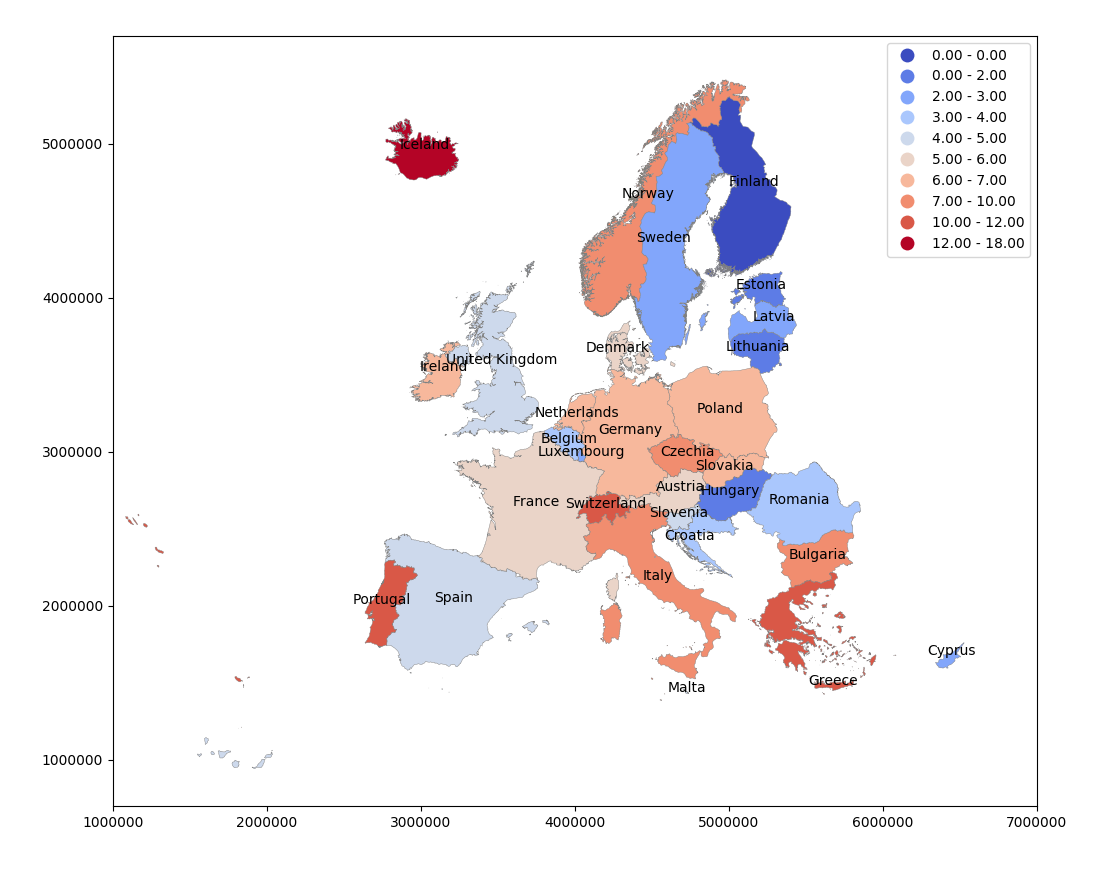
Refer to caption
Figure 1: Influence of various European countries on potato trade between 1973−20191973-2019. The influence of a country is measured by the number of its out-neighbors in the learnt game.

In this section, we performed a computational experiment on real world data to demonstrate the effectiveness of our method. We used our method to identify a set of European countries which have influenced potato trade within Europe between 1973−20191973-2019. The trading interactions among various countries can be modeled as a non-parametric strategic game among self-interested countries.

Our experiments were conducted on the publicly available potato trade data from https://ec.europa.eu/eurostat/web/agriculture/data/database. We extracted the potato trade data among n=31n=31 European countries between 19731973 to 20192019. Each training sample corresponds to a year, and thus, we had T=47T=47 samples for our experiments. The dataset contains the country-wise production volume of potato for 4747 years which we treated as the action xx of players. The dataset also contains country-wise trade prices of potato for 4747 years which we treated as payoff u~i​(x)\widetilde{u}_{i}(x) for each country. We chose r=16r=16 basis functions for the Fourier series expansion of each pairwise utility function to run our experiments. In particular, for each pairwise utility function u¯i​j​(xi,xj),∀i,j∈{1,…,n},i≠j\widebar{u}_{ij}(x_{i},x_{j}),\forall i,j\in\{1,\dots,n\},i\neq j, we chose the basis functions from the following set:

ψk(xi,xj)∈⋃l,m∈{1,2}{cos(2πlxi)cos(2πmxj),cos(2πlxi)sin(2πmxj),sin(2πlxi)cos(2πmxj),sin(2πlxi)sin(2πmxj)}\displaystyle\begin{split}\psi_{k}(x_{i},x_{j})\in\bigcup_{l,m\in\{1,2\}}&\{\cos(2\pi lx_{i})\cos(2\pi mx_{j}),\cos(2\pi lx_{i})\sin(2\pi mx_{j}),\sin(2\pi lx_{i})\cos(2\pi mx_{j}),\\ &\sin(2\pi lx_{i})\sin(2\pi mx_{j})\}\end{split} (94)

We computed the influence of the countries by first learning the global graphical game and then computing the number of out-neighbors for each country in the learnt game. The results are shown in Figure 1. We observe that many of the central and southern European countries along with Iceland and Portugal have had high influence in the European potato market .