Using gradient directions to get global convergence of Newton-type methods
Abstract
The renewed interest in Steepest Descent (SD) methods following the work of
Barzilai and Borwein [2] has driven us to consider a globalization strategy based on SD,
which is applicable to any line-search method.
In particular, we combine Newton-type directions
with scaled SD steps to have suitable descent directions.
Scaling the SD directions with a suitable step length makes
a significant difference with respect to similar globalization approaches,
in terms of both theoretical features and computational behavior. We apply our strategy to Newton’s method
and the BFGS method, with computational results that appear interesting
compared with the results of well-established globalization strategies devised ad hoc for those methods.
AMS subject classification: 65K05, 90C30, 49M15.
Keywords:
Newton-type methods, globalization strategies, steepest descent step.1 Introduction
We are concerned with the following optimization problem:
| (1) |
where is twice continuously differentiable. Hereafter and denote the gradient and the Hessian of , respectively.
A strictly monotone line-search method for solving (1) generates a sequence as follows:
| (2) |
where is a descent direction, is a step length and . For simplicity of notation, we define , and . The direction must be of strict descent, i.e.,
| (3) |
However, condition (3) alone does not ensure convergence, and must satisfy, e.g., the angle criterion
| (4) |
where the sequence is bounded away from 0, which means that the angle between the search direction and the Steepest Descent (SD) direction must be bounded away from the right angle.
The step length must usually satisfy the Armijo condition
| (5) |
or the Wolfe conditions, i.e., (5) and
| (6) |
We note that (5) forces a sufficient decrease in the objective function, while the curvature condition (6) prevents the method from taking too small steps, which is not guaranteed by condition (5) alone. This drawback can be avoided by choosing with a suitable backtracking procedure [25, page 37].
In a Newton-type (NT) method, the search direction is computed as the solution of the linear system
| (7) |
where is some symmetric matrix, possibly positive definite so that (3) automatically holds. With the choice , where is the identity matrix, the NT method reduces to the classical SD method, which is globally convergent with at most linear rate. Recently, several attempts have been made to get more efficient SD methods. In particular, starting from the seminal work by Barzilai and Borwein (BB) [2], it has been observed that appropriate choices of can, to some extent, remedy the slow convergence of the SD method, even for the solution of constrained problems by gradient projection strategies. This led to effective algorithms [6, 10, 12, 27, 28], which have been successfully used in several applications [1, 8, 9, 14, 31].
With the inclusion of second-order information through we expect a better rate of convergence. However, the search direction does not guarantee global convergence, even if is positive definite for each . An example is provided by the classical Newton’s method, where . If solves (1), with positive definite, and is Lipschitz continuous around , Newton’s method has local, but not global, convergence with quadratic rate [16]. However, a suitable reduction of the Newton step allows global convergence in the convex case (see, e.g., [24, page 34]). In the nonconvex case the Newton direction may not be a descent direction. Therefore, modifications of Newton’s method have been developed that replace by , where is a symmetric matrix such that is positive definite [22] and the solution of is a descent direction at . We will refer to these methods as Modified Newton’s (MN) methods. This approach can be extended to the general framework of Newton-type methods, in which, given an approximation of , one may consider a matrix such that is “sufficiently positive definite” and is not much larger than for some norm [15]. If the eigenvalues of are bounded away from zero independently of and the Armijo condition is satisfied by backtracking, then all limit points of the method using the directions obtained by solving (7) with are stationary for (1)[3, 23]. The most successful and well-established algorithms for the computation of are based on modified Cholesky factorizations of the matrix [15]. Another possibility is setting , where is a suitable constant, so that the search direction is
| (8) |
For quasi-Newton methods ad-hoc globalization strategies have been proposed which avoid matrix factorizations. Next, we briefly describe some of them for the BFGS method [16]. In this case
| (9) |
with solution of the system
| (10) |
where the matrix is updated by the formula
| (11) |
with and .
For convex optimization problems it can be shown that, under suitable hypotheses, the BFGS method with a line search satisfying the Wolfe conditions is globally convergent and locally superlinearly convergent [4]. For nonconvex functions Dai [7] showed with an example that the BFGS with Wolfe line search may fail. Later on Mascharenhas [20] showed that the BFGS method, as well as other methods in the Broyden class, may fail for nonconvex objective functions when an exact line search is used.
For nonconvex minimization problems Li and Fukushima [18] proposed a modified version of BFGS, called MBFGS, using an Armijio line search or a Wolfe one, and based on an update formula for the matrix in (10), which is equal to (11) with replaced by
| (12) |
where
| (13) |
This update formula guarantees that [18, Section 5]
and therefore is positive definite, provided is positive definite, thus ensuring that the descent condition holds. The update formula (13) was inspired by the MN method with search direction
| (14) |
where is a regularization parameter. The MBFGS method with Armijo or Wolfe line search is globally convergent even for nonconvex problems [18].
Later on, the same authors proposed the following BFGS formula with cautious update rule [19]:
| (15) |
where and are positive constants, and for which global convergence was proved without convexity assumptions.
In this paper we consider a globalization approach applicable to any Newton-type method. The basic idea consists of linearly combining the NT and SD directions. The goal is to bring the iterates sufficiently close to a solution through the globally convergent SD method, so that once the iterates are in the basin of attraction of the NT method, it can lead to faster convergence than SD. Although this approach is not new (see, e.g., [29, 30, 17] and [3, Section 1.4.4]) and much simpler than those based on trust regions and incomplete factorizations, it has been little utilized, likely because of little confidence in the SD method. Here we show that a hybrid strategy which combines SD and NT directions can give very interesting numerical results. In our opinion, a suitable scaling of the SD direction is a key issue in making this approach effective. We also find that, besides fostering global convergence, this strategy can be effective in speeding up NT methods.
This article is organized as follows. In Section 2 we present our globalization strategy, and how the coefficient governing the linear combination can be computed. Section 3 deals with the convergence of the resulting algorithm, in particular for Newton’s method. In Section 4 we discuss results of numerical experiments carried out with our algorithm using either Newton’s or the BFGS method, including a comparison with some benchmarks algorithms. We conclude in Section 5.
2 Globalization strategy
We propose a line-search method of the form (2), where is the NT direction if the angle criterion (4) is satisfied, otherwise
| (16) |
with and . A sketch of this method, which we call SD Globalized (SDG) line-search method, is provided in Algorithm 1.
Regarding the NT direction (7), which can be, e.g., a Newton, quasi-Newton or inexact Newton direction, we assume that it is well-scaled, so that we scale only the SD direction through . The search direction (16) is closely related to the one proposed by Shi in [29, 30], which is defined as
| (17) |
Notice that, unlike (17), the search direction (16) is invariant to the scaling of the objective function, as long as is invariant (e.g., when is a BB step length and ).
The next theorem shows how to compute values of guaranteeing that (16) satisfies (4). We note that the first part slightly generalizes Lemma 2.1 in [29].
Theorem 1
Let us consider any and , and assume that
| (18) |
with solution of system (7) where is any symmetric matrix not multiple of .
- i)
Let be the smallest root in of the polynomial
(19) where
If is defined according to (16) with , then
- ii)
- iii)
A lower bound for is provided by the value defined as
(21) where
(22)
Proof
We first prove that is well defined. Let us consider
which is a continuous function of . Note that is the cosine of the angle between the antigradient and the direction
which spans continuously the cone between , corresponding to , and the vector , corresponding to . From its definition it is clear that is a monotonically decreasing function in the interval . Since
has a unique zero in . The solutions of the equation
| (23) |
are the solutions of . By simple computations, it is easy to verify that the solutions of (23) are the roots of the polynomial (19). Now we observe that . To conclude the proof of item i) we need to analyze the two possible cases about the sign of
Item ii) of the theorem comes from the observation that is a monotonically decreasing function in , which implies that for all .
To prove item iii), we note that the search direction (16) satisfies (20) if and only if
| (24) |
Since
a sufficient condition for (24) to hold is that
| (25) |
This condition gives us a way to compute a lower bound for . By straightforward computations one can check that (25) is equivalent to
i.e.,
| (26) |
where and are defined in (22). We observe that (18) implies and comes from the definition of and . Therefore, we have that (26) holds if and only if . Item ii) implies .
Remark 1
Items i) and iii) of the previous theorem suggest two choices for the coefficient in (16), namely and . Note that is the largest value of such that the angle criterion (20) is satisfied. Moreover, by looking at the definition of in (22) we can easily find a relation between the “quality” of the NT direction and the value of . We can indeed write as
i.e., provides a measure of the violation of the angle criterion (20). If approaches , we have that tends to zero and tends to , allowing us to take a direction close to the NT one. Conversely, if approaches , the value of may increase, implying a decrease of and thus fostering the descent direction to be close to the SD direction.
Going back to the classical globalization strategies mentioned in the previous section, we note that the search direction
| (27) |
where , is based on the following quadratic approximation of at :
| (28) |
in which the role of is to guarantee that the model be “sufficiently” convex. Our approach is based on a different second-order model, namely
where
| (29) |
Even when is not positive definite, the choice of guarantees that (20) holds for . A simple computation shows that we only require convexity for the univariate function
| (30) |
which attains its minimum at . On the contrary, a globalization strategy like the one based on a shifted linear system of the form (8) forces the overall quadratic model (28) to be convex, potentially leading to a model insufficiently faithful to .
The directions (8) and (16) remind us of Trust Region (TR) methods [5]. These methods compute by minimizing a quadratic model of near ,
| (31) |
where is updated at each iteration to get a “good” approximation of in the ball with center and radius . The point is a minimizer of in this ball if and only if is a solution of the system
| (32) |
for a scalar such that . Therefore, we can regard direction (8) as a TR step. Direction (16) can be also related to the dogleg and the two-dimensional subspace minimization approaches, which provide approximate solutions to the TR subproblem (31) by making a search in the space spanned by the SD and Newton directions (see, e.g., [25]).
As already pointed out, unlike (17), the search direction (16) is invariant to the scaling of the objective function when is invariant. In order to clarify the relevance of this issue, we show a simple numerical example. We consider the so-called “Brown badly-scaled” function [21], defined as
| (33) |
We compare the performances of the line-search methods using as search directions respectively (17) and (16) (with set as the BB2 step length defined in [2, equation (5)]), on scaled versions of (33),
for different values of the scale factor . For both algorithms, is set as the Newton direction. Furthermore, we set for each and as stop condition. Table 1 contains the number of iterations (its) and function evaluations (evals) performed by the SDG method; as expected, when the search directions (17) are used, the performance of the line-search algorithm dramatically depends on the scale factor. On the other hand, the results in Table 1 confirm that the search directions computed using (16) are scale invariant. Notice that the Newton direction is scale invariant, whereas the gradient scales with , so that the larger the scale factor, the closer (17) is to the SD direction. This probably explains why in Table 1 we observe a progressive deterioration of the performance of the search direction (17) when moving from (close to the Newton direction) to (close to the SD direction). Finally, a comparison between the two search directions for demonstrates the importance of a suitable choice of in the hybrid strategy (note that in (17) it is always ).
3 Convergence
We now focus on the convergence properties of the SDG method. The theorems in this section are a slight modification of results presented by the authors in [11].
Theorem 2
Let and assume that is bounded away from . Then, for any , the limit points of the sequence generated by Algorithm 1 are stationary.
Proof
Let . At any iteration , Theorem 1 guarantees the existence of a coefficient for step 9 of Algorithm 1, therefore a direction satisfying can be found. Since the sequence is bounded from below by and is obtained by a backtracking technique to fulfill condition (5), the thesis follows from [3, Proposition 1.2.1].
The next theorem shows that the SDG method has quadratic convergence rate when the direction is the Newton direction. The proof is omitted because it is practically the same as the proof of Theorem 2 in [11].
Theorem 3
Let and let be generated by the SDG method where is the Newton direction. Let in (5) be such that and the sequence be nonincreasing with limit . Suppose also that there exists a limit point of where is positive definite and is Lipschitz continuous around . If is sufficiently small, then converges to with quadratic rate.
4 Computational experiments
We implemented two MATLAB versions of the SDG algorithm, using Newton’s method and the BFGS method, and compared them with the Modified Newton method using a modified Cholesky factorization [15] and with the CBFGS method [19], respectively. To better understand the effect of our globalization strategy, we also run Newton’s method, the BFGS method, and the SD one with the BB2 Barzilai-Borwein step length used in the numerical example at the end of Section 2.
In the SDG and pure SD methods, we set , if , and otherwise; here is the BB2 step length, and . We chose BB2 instead of other BB step lengths (see, e.g., [10]) because BB2 was more effective in preliminary numerical experiments. The Hessian approximations in SDG with BFGS, in BFGS and in CBFGS were initialized as explained in [25, page 143]. We applied a shrinking strategy for the selection of in (20): given and , at the -th iterate () we set if , and otherwise. To prevent the sequence from going toward zero, we set a threshold for equal to , where is the machine epsilon. It is worth noting that in none of the tests performed the value of reached the threshold. In all the algorithms, the Armijo backtracking line search with (see (5)) and quadratic interpolation [25, Section 3.5] was performed. The methods were stopped as soon as
| (34) |
with ; as a safeguard we also stopped the execution when a maximum number, , of 2000 iterations was achieved or the objective function appeared to get stuck, i.e.,
Algorithm 2 is a detailed version of Algorithm 1 that includes implementation details. By numerical experiments we found that the use of the pure SD direction with BB2 step length is computationally convenient when is not a descent direction (see lines 12-13). The notation SDG[NT,] highlights that the algorithm uses a selected NT method (e.g., Newton’s or BFGS) and as initial value of the sequence .
All the experiments were carried out using MATLAB R2018b. Comparisons were performed by using the performance profiles introduced in [13], which are briefly described next for completeness.
Let be a statistic corresponding to the solution of a test problem by an algorithm , and suppose that the smaller the statistic the better the algorithm. Furthermore, let be the smallest value attained on the test by one of the algorithms under analysis. The performance profile of the algorithm is defined as
where the ratio is set to if algorithm fails in solving . In other words, is the fraction of problems for which is within a factor of the smallest value . Thus is the percentage of problems for which is the best, while gives the percentage of problems that are successfully solved by .
The performance profiles considered in this work use as performance statistics the number of iterations and the number of function evaluations. We note that in Section 4.2.2, in comparing our SDG algorithm based on Newton’s method with an MN method, we do not consider the execution time because the MN implementation exploits a C code for the modified Cholesky factorization, called via a MATLAB mex file, while the Newton systems in the SDG algorithm are solved by the MATLAB function backslash. Thus, in this case a time comparison would be unfair. In all the other experiments the algorithms compared have about the same cost per iteration, therefore using the number of iterations as performance statistic appears sensible. Furthermore, the number of objective function evaluations is related to the number of line searches performed, and provides also information on the quality of the descent direction. Nevertheless, we use a performance profile based on the execution time at the end of Section 4.2.2, to further support some results.
To better show the effectiveness of the proposed strategy, we considered two sets of test problems, described in the following section.
4.1 Test problems
4.1.1 Nonconvex problems
We considered 36 problems available from https://people.sc.fsu.edu/˜jburkardt/m_src/test_opt/test_opt.html, including the unconstrained minimization problems from the Moré-Garbow-Hillstrom collection [21] and other problems. We set the problem size equal to 100 for all the problems where the dimension could be chosen by the user. For each problem we used 10 starting points, i.e., the point provided with the problem and the points , with , where , was a random number in , , and the values were logarithmically spaced in the interval . These choices resulted in a set of 360 nonconvex optimization problem instances.
4.1.2 Convex problems coming from machine learning
The second set of test problems consists in the minimization of convex functions arising from machine learning. In particular, given pairs , where and , we considered the problem of training a linear classifier by minimizing the function
| (35) |
where and .
1 - https://www.csie.ntu.edu.tw/˜cjlin/libsvmtools/datasets/,
2 - http://www.ics.uci.edu/˜mlearn/MLRepository.html,
3 - NAACCR Incidence - CiNA Public File, 1995-2015, North American Association of Central Cancer Registries,
4 - http://yann.lecun.com/exdb/mnist.
| name | points | features |
|---|---|---|
| a6a11footnotemark: 1 | 11220 | 123 |
| a7a11footnotemark: 1 | 16100 | 123 |
| a8a11footnotemark: 1 | 22696 | 123 |
| a9a11footnotemark: 1 | 32561 | 123 |
| adult22footnotemark: 2 | 48842 | 122 |
| cina33footnotemark: 3 | 16033 | 132 |
| cod-rna11footnotemark: 1 | 59535 | 8 |
| ijcnn111footnotemark: 1 | 49990 | 22 |
| mnist44footnotemark: 4 | 7603 | 100 |
| mushrooms11footnotemark: 1 | 8124 | 112 |
| phishing11footnotemark: 1 | 11055 | 68 |
| w6a11footnotemark: 1 | 17188 | 300 |
| w7a11footnotemark: 1 | 24692 | 300 |
| w8a11footnotemark: 1 | 49749 | 300 |
We considered 14 datasets, whose dimensions and sources are reported in Table 2. For each dataset we considered a 10-fold cross validation setting, thus obtaining 10 different training problems of the form (35) with approximately equal to 0.9 times the total number of points. For each problem we set , which is a choice usually found in literature. This produced a total of 140 instances for training our strategy. For this set of test problems we focused on the BFGS method.
4.2 Numerical results
4.2.1 Comparison on the choice of
First, we focused on the choice of in (16). Theorem 1 suggests and as two possible alternatives. Just to get a first picture, we considered the so-called “Gulf research and developement” function [21], defined as
with starting point . We ran SDG[Newton,0.5] with and computed also at each iteration. The values of and are shown in the top plot in Figure 1, for the iterations in which the Newton step was rejected as a search direction. For the same iterations, in the bottom plot we depicted the values of for in (16), computed with , and (the last one corresponds to the pure Newton’s method). This example suggests that the difference between and is negligible, especially when close to the solution. Conversely, the angle between (computed with either or ) and is non-negligible, especially far from the solution.
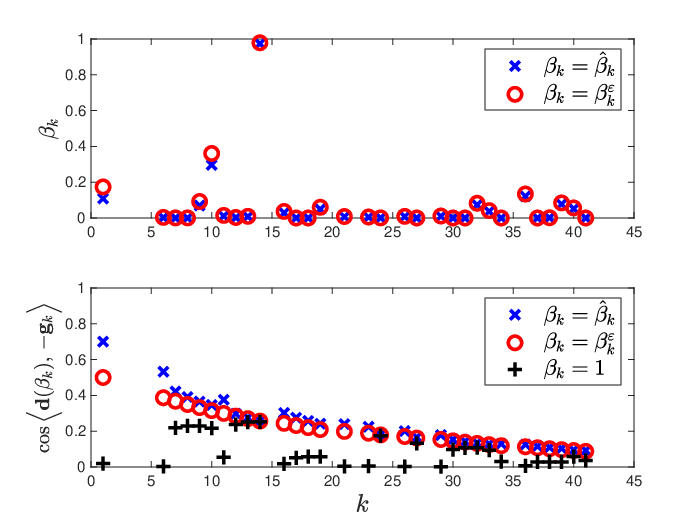
Then we ran two versions of SDG[Newton,0.5], with and , on the solution of the 360 nonconvex problem instances previously described, looking for experimental evidence about the choice of . Since the problems are nonconvex, different algorithms may reach different local minima starting from the same point. We noted that, out of the 360 considered problem instances, SDG went to the smallest local minimum 267 times with , and 295 times with . To have a fair picture, we compared the two versions of SDG on the 202 instances where they reached equal solutions (two solutions were considered equal if they coincided up to the third significant digit). The performance profiles reported in Figure 2 show a comparison in terms of number of iterations (left) and number of objective function evaluations (right), and suggest that is preferable to . If we had to venture a guess, based on our experience, we would say that far from the solution can be significantly smaller then , and this increases the SD component in (16). Far from the solution, the SD direction with a suitable step length like BB2 can even be more effective than Newton’s method in decreasing the objective function, and this might explain, to some extent, the results in Figure 2.


We also compared SDG[BFGS,0.5] with and on the first set of test problems. In this case, the two versions of SDG computed the same solution on 148 problem instances. As shown by the performance profiles in Figure 3, the implementation with slightly outperformed the one with .


A similar analysis was carried out for the convex problems from machine learning, comparing the versions SDG[BFGS,0.5] with the two different values of . Again, seems to provide the best results, in terms of both number of iterations and number of function evaluations, as shown in Figure 4. Therefore, we decided to set in the remaining numerical experiments.


4.2.2 Comparison with other globalization strategies
To perform a comparison with other globalization strategies, we ran, on the nonconvex problems, the SDG[Newton,0.5] method and an MN method based on the modified Cholesky factorization GMW-II [15] (see https://github.com/hrfang/mchol). For completeness, we also ran Newton’s method.
We found that Newton’s method with line search stopped without satisfying criterion (34) for 168 out of 360 problem instances. Conversely, MN failed only on 10 instances, whereas SDG[Newton,0.5] was always able to satisfy (34) within 2000 iterations. Figure 5 summarizes the results of the comparison between SDG[Newton,0.5] and the Modified Newton’s method for the 134 problem instances in which the methods obtained the same solution. The profiles show that our algorithm required less function evaluations, although it was slightly less efficient in terms of iterations.


We also compared SDG[BFGS,0.5] with CBFGS using (see (15)) and with BFGS. The performance profiles in Figure 6 show how SDG[BFGS,0.5] compares with CBFGS and BFGS in the solution of the 221 problem instances in which the algorithms get the same solution. Note that CBFGS and BFGS overlap extensively. In other words, BFGS does not seem to really need a globalization strategy, and the cautious update rule (15) is likely to reduce to the standard BFGS update rule almost always. Figure 6 also shows that our globalization strategy can slightly improve the performance of the BFGS method.


With the aim of better understanding the behavior of SDG[BFGS,0.5], in Figure 7 we plotted the sequence for two representative instances of nonconvex problems. We set when the BFGS direction was accepted (see lines 7-8 of Algorithm 2), and when the SD direction scaled by the BB2 step length was selected (see lines 12-13 of Algorithm 2).

In the top plot, concerning a very easy problem (the Goldstein-Price polynomial), we see that the method practically switches from SD to BFGS at the third iteration. The bottom plot, concerning the extended Rosenbrock parabolic valley function, shows that in the very first iterations it is likely that is close to 0, and the SD component is dominating the search direction (16). As the number of iterations increases, the SD component in (16) becomes smaller and smaller, and eventually the method reduces to BFGS.
Concerning the convex problems, we considered BFGS only, i.e., we compared SDG[BFGS,0.5], CBFGS and BFGS. Figure 8 confirms the trend already observed in the nonconvex case: the CBFGS and BFGS methods behave the same way, and SDG[BFGS,0.5] outperforms both of them.


The results in the convex case suggest that a suitable linear combination of an NT direction with the SD one can have a beneficial effect in speeding up the convergence, in addition to providing global convergence. To further investigate this issue, we also made computational experiments with SDG[BFGS,0.9] on the convex test problems. Of course, the choice favors the SD component in the search direction, and we cannot suggest it as a safe choice in general. However, the comparison with SDG[BFGS,0.5] in Figure 9 shows that for the selected problems SDG[BFGS, 0.9] is more efficient than SDG[BFGS,0.5],and hence than the standard BFGS.


Finally, the performance profiles in Figure 10 show that SDG[BFGS,0.9] generally outperforms the SD method with BB2 step length. This suggests that the good behavior of SDG[BFGS,0.9] does not depend only on the use of SD directions with effective step lengths, but also on the efficient combination of these directions with BFGS ones. This is confirmed by Figure 11, where SDG[BFGS,0.9], BFGS and the SD method with BB2 step length are compared in terms of execution time, showing that the proposed algorithm is more efficient than the others.
5 Conclusions
We proposed a globalization strategy to be used with any NT method, which is based on a linear combination of the NT and SD search directions. Our approach, which generalizes the one proposed in [29, 30], looks easier and more flexible than globalization strategies which have been devised ad hoc for specific methods [15, 19]. We believe that a key issue in our strategy is to take the SD direction with a suitable step length. The reason is twofold: first, from the theoretical point of view, it allows us to have search directions that are invariant to the scaling of the objective function; second, it allows us to inject in the globalized method the proven effectiveness of gradient methods based on particular step-length rules [10]. Our computational experiments suggest that the use of a line search along a suitable linear combination of NT and SD directions can improve numerical performance with respect to the NT method, in addition to providing global convergence. In particular, the SD component with the BB2 step length showed a beneficial effect especially when far from the solution.
Acknowledgments
This work was supported by GNCS-INdAM, Italy, and by the V:ALERE Program of the University of Campania “L. Vanvitelli” under the VAIN-HOPES Project.
References
- [1] L. Antonelli, V. De Simone, and D. di Serafino, On the application of the spectral projected gradient method in image segmentation, Journal of Mathematical Imaging and Vision, 54 (2016), pp. 106–116.
- [2] J. Barzilai and J. M. Borwein, Two-point step size gradient methods, IMA Journal of Numerical Analysis, 8 (1988), pp. 141–148.
- [3] D. P. Bertsekas, Nonlinear Programming, Athena Scientific, second ed., 1999.
- [4] R. H. Byrd, J. Nocedal, and Y.-X. Yuan, Global convergence of a class of Quasi-Newton methods on convex problems, SIAM Journal on Numerical Analysis, 24 (1987), pp. 1171–1190.
- [5] A. R. Conn, N. I. M. Gould, and P. L. Toint, Trust-region methods, MPS-SIAM Series on Optimization, SIAM, 2000.
- [6] S. Crisci, V. Ruggiero, and L. Zanni, Steplength selection in gradient projection methods for box-constrained quadratic programs, Applied Mathematics and Computation, 356 (2019), pp. 312–327.
- [7] Y.-H. Dai, Convergence properties of the BFGS algoritm, SIAM Journal on Optimization, 13 (2002), pp. 693–701.
- [8] R. De Asmundis, D. di Serafino, and G. Landi, On the regularizing behavior of the SDA and SDC gradient methods in the solution of linear ill-posed problems, Journal of Computational and Applied Mathematics, 302 (2016), pp. 81–93.
- [9] D. di Serafino, G. Landi, and M. Viola, ACQUIRE: an inexact iteratively reweighted norm approach for TV-based Poisson image restoration, Applied Mathematics and Computation, 364 (2020), p. 124678.
- [10] D. di Serafino, V. Ruggiero, G. Toraldo, and L. Zanni, On the steplength selection in gradient methods for unconstrained optimization, Applied Mathematics and Computation, 318 (2018), pp. 176–195.
- [11] D. di Serafino, G. Toraldo, and M. Viola, A gradient-based globalization strategy for the Newton method, in Numerical Computations: Theory and Algorithms. NUMTA 2019, Y. D. Sergeyev and D. E. Kvasov, eds., vol. 11973 of Lecture Notes in Computer Science, Springer, 2020, pp. 177–185.
- [12] D. di Serafino, G. Toraldo, M. Viola, and J. Barlow, A two-phase gradient method for quadratic programming problems with a single linear constraint and bounds on the variables, SIAM Journal on Optimization, 28 (2018), pp. 2809–2838.
- [13] E. D. Dolan and J. J. Moré, Benchmarking optimization software with performance profiles, Mathematical Programming, Series B, 91 (2002), pp. 201–213.
- [14] Z. Dostál, G. Toraldo, M. Viola, and O. Vlach, Proportionality-based gradient methods with applications in contact mechanics, in High Performance Computing in Science and Engineering. HPCSE 2017, T. Kozubek, M. Čermák, P. Tichý, R. Blaheta, J. Šístek, D. Lukáš, and J. Jaroš, eds., vol. 11087 of Lecture Notes in Computer Science, Springer, 2018, pp. 47–58.
- [15] H. Fang and D. P. O’Leary, Modified Cholesky algorithms: a catalog with new approaches, Mathematical Programming, 115 (2008), pp. 319–349.
- [16] R. Fletcher, Practical methods of optimization, John Wiley & Sons, second ed., 2000.
- [17] L. Han and M. Neumann, Combining quasi-Newton and Cauchy directions, International Journal of Applied Mathematics, 12 (2003), pp. 167–191.
- [18] D.-H. Li and M. Fukushima, A modified BFGS method and its global convergence in nonconvex minimization, Journal of Computational and Applied Mathematics, 129 (2001), pp. 15–35.
- [19] , On the global convergence of the BFGS method for nonconvex unconstrained optimization problems, SIAM Journal on Optimization, 11 (2001), pp. 1054–1064.
- [20] W. F. Mascarenhas, The BFGS method with exact line searches fails for non-convex objective functions, Mathematical Programming, Series B, 99 (2004), pp. 49–61.
- [21] J. J. Moré, B. S. Garbow, and K. E. Hillstrom, Testing unconstrained optimization software, ACM Transactions on Mathematical Software, 7 (1981), pp. 17–41.
- [22] J. J. Moré and D. C. Sorensen, Newton’s method, in Studies in Numerical Analysis, G. Golub, ed., The Mathematical Association of America, Providence, RI, 1984, pp. 29–82.
- [23] W. Murray, Newton-type methods, in Wiley Encyclopedia of Operations Research and Management Science, Wiley, 2011.
- [24] Y. Nesterov, Introductory lectures on convex optimization. A basic course, vol. 87 of Applied Optimization, Springer Science+Business Media, 2004.
- [25] J. Nocedal and S. J. Wright, Numerical Optimization, Springer Series in Operations Research and Financial Engineering, Springer, second ed., 2006.
- [26] E. Polak, Optimization. Algorithms and consistent approximations, vol. 124 of Applied Mathematical Sciences, Springer, 1997.
- [27] F. Porta, M. Prato, and L. Zanni, A new steplength selection for scaled gradient methods with application to image deblurring, Journal of Scientific Computing, 65 (2015), pp. 895–919.
- [28] L. Pospíšil and Z. Dostál, The projected Barzilai–Borwein method with fall-back for strictly convex QCQP problems with separable constraints, Mathematics and Computers in Simulation, 145 (2018), pp. 79–89.
- [29] Y. Shi, A globalization procedure for solving nonlinear systems of equations, Numerical Algorithms, 12 (1996), pp. 273–286.
- [30] , Globally convergent algorithms for unconstrained optimization, Computational Optimization and Applications, 16 (2000), pp. 295–308.
- [31] R. Zanella, P. Boccacci, L. Zanni, and M. Bertero, Efficient gradient projection methods for edge-preserving removal of Poisson noise, Inverse Problems, 25 (2009), p. 045010.