跳到论文正文
W Papers独立论文阅读器 arXiv:2004.00915 论文正文 计算阅读时间 · 0%
引用这篇论文根据当前论文元数据生成,正式投稿前建议核对。


License: CC BY 4.0
arXiv:2004.00915v1 [eess.SY] 02 Apr 2020

Safe Reinforcement Learning via Projection on a Safe Set: How to Achieve Optimality?

Sebastien Gros    Mario Zanon    Alberto Bemporad Address: Norwegian University of Technology, NTNU Address: IMT School for Advanced Studies Lucca
Abstract

For all its successes, Reinforcement Learning (RL) still struggles to deliver formal guarantees on the closed-loop behavior of the learned policy. Among other things, guaranteeing the safety of RL with respect to safety-critical systems is a very active research topic. Some recent contributions propose to rely on projections of the inputs delivered by the learned policy into a safe set, ensuring that the system safety is never jeopardized. Unfortunately, it is unclear whether this operation can be performed without disrupting the learning process. This paper addresses this issue. The problem is analysed in the context of QQ-learning and policy gradient techniques. We show that the projection approach is generally disruptive in the context of QQ-learning though a simple alternative solves the issue, while simple corrections can be used in the context of policy gradient methods in order to ensure that the policy gradients are unbiased. The proposed results extend to safe projections based on robust MPC techniques.

keywords
Safe Reinforcement Learning, safe projection, robust MPC

1 Introduction

Reinforcement Learning (RL) is a tool for tackling optimal control from data. RL methods seek to increase the closed-loop performance of the control policy deployed on the system as observations are collected. RL methods often rely on Deep Neural Networks (DNN) to carry the policy approximation 𝝅𝜽\boldsymbol{\mathrm{\pi}}_{\boldsymbol{\mathrm{\theta}}}. Control policies based on DNNs provide limited opportunities for formal verifications of the resulting closed-loop behavior, and for imposing hard constraints on the evolution of the state of the real system. The development of safe RL methods is currently an open field of research (J. Garcia 2013).

In order to tackle safety issues in RL, it has been recently proposed, see (Wabersich et al. 2019) and references therein, to use projections of the inputs delivered by the RL policy 𝝅𝜽\boldsymbol{\mathrm{\pi}}_{\boldsymbol{\mathrm{\theta}}} into safe sets, which is known by construction to ensure the safety of the system. The construction of the safe set can, e.g., rely on specific knowledge of the system, or robust model predictive control techniques. The projection then operates as a safeguard that prevents RL from taking unsafe decisions, and adopts the safe decision that is the closest to the RL policy when RL is unsafe.

In this paper, we investigate the interaction between these safe policy projections and the learning process deployed by RL. We show that because the projection modifies the policy developed via RL, it can disrupt the learning process performed such that the learned policy can be suboptimal. The problem occurs both in the context of QQ-learning and policy gradient approaches using actor-critic methods. We then propose simple techniques to alleviate the problem. In the context of QQ-learning, we show that the projection technique in general jeopardizes optimality, as it is the projection of a (possibly) optimal policy on a set, and that the problem is best alleviated by relying on a direct minimization of the QQ function learned by RL, under the safety constraint that the inputs must belong to the safety set, as proposed in (Zanon and Gros 2019). In the context of the deterministic policy gradient approaches, we show that, in order to prevent the projections to bias the policy gradient estimations, the actor-critic method must be corrected with a correction which is simple to deploy. In the context of stochastic policy gradient methods, we show that the actor-critic must be constructed in a particular way to prevent the projection from biasing the policy gradient estimations. We finally show that these results extend to the case of a projection performed via robust Model Predictive Control (MPC) techniques.

The paper is structured as follows. Section 2 provides some background material. Section 3 details the projection approach in the context of QQ-learning, and proposes an approach to address the resulting difficulties. Section 4 details the projection approach for policy gradient methods, both deterministic and stochastic, and proposes simple actor-critic formulations that prevent the projection from biasing the policy gradient estimations. Section 5 extends the results to the case in which the projection is performed via robust MPC. Section 6 proposes a simple simulation example using robust linear MPC in the stochastic policy gradient case, and Section 7 provides conclusions.

2 Background

In the following, we will consider that the dynamics of the real system are possibly stochastic, evolving on continuous state-input spaces. We will furthermore consider stochastic policies π\pi, taking the form of conditional probability densities π⁡[𝐮|𝐱]:ℝm×ℝn→ℝ+,{\pi}\left[\boldsymbol{\mathrm{u}}\,|\,\boldsymbol{\mathrm{x}}\right]\,:\,\mathbb{R}^{m}\times\mathbb{R}^{n}\rightarrow\mathbb{R}_{+}, denoting the probability density of selecting a given input 𝐮\boldsymbol{\mathrm{u}} when the system is in a given state 𝐱\boldsymbol{\mathrm{x}}. We will also consider deterministic policies 𝝅⁡(𝐱):ℝn→ℝm\boldsymbol{\mathrm{\pi}}\left(\boldsymbol{\mathrm{x}}\right)\,:\,\mathbb{R}^{n}\rightarrow\mathbb{R}^{m} delivering 𝐮\boldsymbol{\mathrm{u}} as a function of 𝐱\boldsymbol{\mathrm{x}}. For a given stage cost L⁡(𝐱,𝐮)∈ℝn×ℝm→ℝL(\boldsymbol{\mathrm{x}},\boldsymbol{\mathrm{u}})\in\mathbb{R}^{n}\times\mathbb{R}^{m}\rightarrow\mathbb{R} and a discount factor γ∈[0,1]\gamma\in[0,1], the performance of a policy π\pi is assessed via the total discounted expected cost

J(π)=𝔼π[∑k=0∞γkL(𝐱k,𝐮k)|𝐮k∼π[⋅|𝐱k]],\displaystyle J(\pi)=\mathbb{E}_{{\pi}}\left[\left.\sum_{k=0}^{\infty}\,\gamma^{k}L(\boldsymbol{\mathrm{x}}_{k},\boldsymbol{\mathrm{u}}_{k})\,\right|\,\boldsymbol{\mathrm{u}}_{k}\sim\pi\left[\,\cdot\,|\,\boldsymbol{\mathrm{x}}_{k}\right]\,\right], (1)

where 𝔼π\mathbb{E}_{{\pi}} is the expected value of the closed-loop trajectories under policy π\pi, including the initial conditions 𝐱0\boldsymbol{\mathrm{x}}_{0}.

In the deterministic policy case, the policy in (1) takes the form of a Dirac distribution centered at 𝝅\boldsymbol{\mathrm{\pi}}. The optimal policy associated to the state transition, the stage cost LL and the discount factor γ\gamma is deterministic and given by

𝝅⋆=arg​min𝝅⁡J⁡(𝝅).\displaystyle\boldsymbol{\mathrm{\pi}}_{\star}=\mathrm{arg}\min_{\boldsymbol{\mathrm{\pi}}}\,J(\boldsymbol{\mathrm{\pi}}). (2)

Reinforcement Learning seeks to find the parameters 𝜽\boldsymbol{\mathrm{\theta}} such that the parametrized policies 𝝅𝜽\boldsymbol{\mathrm{\pi}}_{\boldsymbol{\mathrm{\theta}}} or π𝜽\pi_{\boldsymbol{\mathrm{\theta}}} approximate closely 𝝅⋆\boldsymbol{\mathrm{\pi}}_{\star}, using observed state transitions. QQ-learning methods build the optimal policy approximation indirectly, as the minimizer (Sutton and Barto 2018):

𝝅𝜽​(𝐱)=arg​min𝐮​Q𝜽​(𝐱,𝐮),\displaystyle{\boldsymbol{\mathrm{\pi}}}_{\boldsymbol{\mathrm{\theta}}}\left(\boldsymbol{\mathrm{x}}\right)=\mathrm{arg}\min_{\boldsymbol{\mathrm{u}}}Q_{\boldsymbol{\mathrm{\theta}}}\left(\boldsymbol{\mathrm{x}},\boldsymbol{\mathrm{u}}\right), (3)

where Q𝜽Q_{\boldsymbol{\mathrm{\theta}}} is an approximation of the true optimal action value function Q⋆Q_{\star}, solution of the Bellman equations (Bertsekas 2007):

V⋆​(𝐱)\displaystyle V_{\star}\left(\boldsymbol{\mathrm{x}}\right) =min𝐮⁡Q⋆​(𝐱,𝐮),\displaystyle=\min_{\boldsymbol{\mathrm{u}}}Q_{\star}\left(\boldsymbol{\mathrm{x}},\boldsymbol{\mathrm{u}}\right), (4a)
Q⋆​(𝐱,𝐮)\displaystyle Q_{\star}\left(\boldsymbol{\mathrm{x}},\boldsymbol{\mathrm{u}}\right) =L(𝐱,𝐮)+γ𝔼[V⋆(𝐱+)|𝐱,𝐮].\displaystyle=L(\boldsymbol{\mathrm{x}},\boldsymbol{\mathrm{u}})+\gamma\mathbb{E}\left[V_{\star}(\boldsymbol{\mathrm{x}}_{+})\,|\,\boldsymbol{\mathrm{x}},\,\boldsymbol{\mathrm{u}}\right]. (4b)

The approximation Q𝜽≈Q⋆Q_{\boldsymbol{\mathrm{\theta}}}\approx Q_{\star} is built using Temporal-Difference or Monte-Carlo techniques.

In contrast, policy gradient techniques manipulate directly the policy parameters according to the policy gradients ∇𝜽J\nabla_{\boldsymbol{\mathrm{\theta}}}J (Sutton et al. 1999). Actor-critic techniques evaluate the policy gradient resulting from a stochastic policy as (Sutton et al. 1999)

∇𝜽J​(π𝜽)=𝔼⁡[∇𝜽​log​π𝜽​[𝐮|𝐱]​Aπ𝜽​(𝐱,𝐮)],\displaystyle\nabla_{\boldsymbol{\mathrm{\theta}}}J(\pi_{\boldsymbol{\mathrm{\theta}}})=\mathbb{E}\left[\nabla_{\boldsymbol{\mathrm{\theta}}}\log\pi_{\boldsymbol{\mathrm{\theta}}}[\boldsymbol{\mathrm{u}}\,|\,\boldsymbol{\mathrm{x}}]A_{\pi_{\boldsymbol{\mathrm{\theta}}}}\left(\boldsymbol{\mathrm{x}},\boldsymbol{\mathrm{u}}\right)\right], (5)

where Aπ𝜽A_{\pi_{\boldsymbol{\mathrm{\theta}}}} is the advantage function associated to the policy π𝜽\pi_{\boldsymbol{\mathrm{\theta}}}, defined as

Aπ𝜽​(𝐱,𝐮)\displaystyle A_{\pi_{\boldsymbol{\mathrm{\theta}}}}\left(\boldsymbol{\mathrm{x}},\boldsymbol{\mathrm{u}}\right) =Qπ𝜽​(𝐱,𝐮)−Vπ𝜽​(𝐱),\displaystyle=Q_{\pi_{\boldsymbol{\mathrm{\theta}}}}\left(\boldsymbol{\mathrm{x}},\boldsymbol{\mathrm{u}}\right)-V_{\pi_{\boldsymbol{\mathrm{\theta}}}}\left(\boldsymbol{\mathrm{x}}\right), (6)

and where

Vπ𝜽​(𝐱)\displaystyle V_{\pi_{\boldsymbol{\mathrm{\theta}}}}\left(\boldsymbol{\mathrm{x}}\right) =𝔼[L(𝐱,𝐮)+γVπ𝜽(𝐱+)|𝐱,𝐮],\displaystyle=\mathbb{E}\left[L(\boldsymbol{\mathrm{x}},\boldsymbol{\mathrm{u}})+\gamma V_{\pi_{\boldsymbol{\mathrm{\theta}}}}(\boldsymbol{\mathrm{x}}_{+})\,|\,\boldsymbol{\mathrm{x}},\,\boldsymbol{\mathrm{u}}\right], (7a)
Qπ𝜽​(𝐱,𝐮)\displaystyle Q_{\pi_{\boldsymbol{\mathrm{\theta}}}}\left(\boldsymbol{\mathrm{x}},\boldsymbol{\mathrm{u}}\right) =L(𝐱,𝐮)+γ𝔼[Vπ𝜽(𝐱+)|𝐱,𝐮],\displaystyle=L(\boldsymbol{\mathrm{x}},\boldsymbol{\mathrm{u}})+\gamma\mathbb{E}\left[V_{\pi_{\boldsymbol{\mathrm{\theta}}}}(\boldsymbol{\mathrm{x}}_{+})\,|\,\boldsymbol{\mathrm{x}},\,\boldsymbol{\mathrm{u}}\right], (7b)

are the value and action-value functions associated to π𝜽\pi_{\boldsymbol{\mathrm{\theta}}}.

Similarly, the policy gradient ∇𝜽J​(𝝅𝜽)\nabla_{\boldsymbol{\mathrm{\theta}}}J(\boldsymbol{\mathrm{\pi}}_{\boldsymbol{\mathrm{\theta}}}) associated to a deterministic policy 𝝅𝜽\boldsymbol{\mathrm{\pi}}_{\boldsymbol{\mathrm{\theta}}} reads as (Silver et al. 2014)

∇𝜽J​(𝝅𝜽)=𝔼⁡[∇𝜽𝝅𝜽​(𝐱)​∇𝐮A𝝅𝜽​(𝐱,𝝅𝜽​(𝐱))],\displaystyle\nabla_{\boldsymbol{\mathrm{\theta}}}J(\boldsymbol{\mathrm{\pi}}_{\boldsymbol{\mathrm{\theta}}})=\mathbb{E}\left[\nabla_{\boldsymbol{\mathrm{\theta}}}\boldsymbol{\mathrm{\pi}}_{\boldsymbol{\mathrm{\theta}}}(\boldsymbol{\mathrm{x}})\nabla_{\boldsymbol{\mathrm{u}}}A_{\boldsymbol{\mathrm{\pi}}_{\boldsymbol{\mathrm{\theta}}}}\left(\boldsymbol{\mathrm{x}},\boldsymbol{\mathrm{\pi}}_{\boldsymbol{\mathrm{\theta}}}(\boldsymbol{\mathrm{x}})\right)\right], (8)

where the advantage function A𝝅𝜽A_{\boldsymbol{\mathrm{\pi}}_{\boldsymbol{\mathrm{\theta}}}} is defined by (6)-(7) taken over a Dirac-like policy density corresponding to a deterministic policy. The advantage functions Aπ𝜽A_{\pi_{\boldsymbol{\mathrm{\theta}}}} and A𝝅𝜽A_{\boldsymbol{\mathrm{\pi}}_{\boldsymbol{\mathrm{\theta}}}} can be estimated using Temporal-Difference or Monte-Carlo techniques.

In the context of Reinforcement-Learning, enforcing the safety of the inputs generated by a policy is not trivial (J. Garcia 2013). Indeed, for safety-critical systems, discovering unsafe inputs from experiments is overly costly, and is typically rather done in extensive simulation campaigns. As an alternative, recent publications have proposed to approach the safety problem underlying RL by adding a safety layer to the RL process, which serves as a safeguard to the policy, see (Wabersich et al. 2019) and references therein. We detail that approach next.

2.1 Safe Policy

In this paper, we consider Reinforcement Learning subject to safety limitations. More specifically, we will consider constraints:

𝐡⁡(𝐱,𝐮)≤0\displaystyle\boldsymbol{\mathrm{h}}\left(\boldsymbol{\mathrm{x}},\boldsymbol{\mathrm{u}}\right)\leq 0 (9)

that must be respected at all time in order for the system safety to be ensured. Moreover, we will consider a (possibly) state-dependent safe set 𝕊⁡(𝐱)\mathbb{S}\left(\boldsymbol{\mathrm{x}}\right) such that

𝐮k∈𝕊⁡(𝐱k),∀k,\displaystyle\boldsymbol{\mathrm{u}}_{k}\in\mathbb{S}\left(\boldsymbol{\mathrm{x}}_{k}\right),\qquad\forall\,k, (10)

entails that (9) is satisfied at all times. We ought to stress here the difference between (9) and 𝕊⁡(𝐱)\mathbb{S}\left(\boldsymbol{\mathrm{x}}\right). Satisfying (9) at time kk entails that the system is safe at that time kk, while 𝕊\mathbb{S} is such that enforcing (10) at time kk entails that the system safety can be guaranteed at all time in the future. In the following, we will assume that 𝕊\mathbb{S} can be described via inequality constraints on 𝐬\boldsymbol{\mathrm{s}}, typically different than 𝐡\boldsymbol{\mathrm{h}}:

𝕊⁡(𝐱)={𝐮|𝐬⁡(𝐱,𝐮)≤0}.\displaystyle\mathbb{S}\left(\boldsymbol{\mathrm{x}}\right)=\left\{\,\boldsymbol{\mathrm{u}}\,\,\,|\,\,\,\boldsymbol{\mathrm{s}}\left(\boldsymbol{\mathrm{x}},\boldsymbol{\mathrm{u}}\right)\leq 0\right\}. (11)

Set 𝕊⁡(𝐱)\mathbb{S}\left(\boldsymbol{\mathrm{x}}\right) can be complex and non-convex. Let us additionally label 𝕏\mathbb{X} the set of states 𝐱\boldsymbol{\mathrm{x}} such that 𝕊⁡(𝐱)\mathbb{S}\left(\boldsymbol{\mathrm{x}}\right) is non-empty, and 𝕎={𝐱,𝐮|𝐬(𝐱,𝐮)≤0}\mathbb{W}=\left\{\,\boldsymbol{\mathrm{x}},\boldsymbol{\mathrm{u}}\,\,\,|\,\,\,\boldsymbol{\mathrm{s}}\left(\boldsymbol{\mathrm{x}},\boldsymbol{\mathrm{u}}\right)\leq 0\right\}. In some applications, the safe set 𝕊\mathbb{S} can be computed explicitly using reachability analysis, but that can be prohibitively difficult in general. Inner convex approximations can then be needed. An approach based on an implicit representation has been the object of recent publications (Zanon and Gros 2019; Gros and Zanon 2020).

Assuming that a safe set 𝕊\mathbb{S} is available, a natural approach to ensure the feasibility of a policy 𝝅𝜽{\boldsymbol{\mathrm{\pi}}}_{\boldsymbol{\mathrm{\theta}}} learned via Reinforcement Learning techniques is to perform a projection into the safe set 𝕊\mathbb{S}, i.e., to solve online the problem:

𝝅𝜽⟂​(𝐱)=arg​min𝐮\displaystyle\boldsymbol{\mathrm{\pi}}_{\boldsymbol{\mathrm{\theta}}}^{\perp}\left(\boldsymbol{\mathrm{x}}\right)=\mathrm{arg}\min_{\boldsymbol{\mathrm{u}}} 12​‖𝐮−𝝅𝜽​(𝐱)‖2\displaystyle\quad\frac{1}{2}\|\boldsymbol{\mathrm{u}}-{\boldsymbol{\mathrm{\pi}}}_{\boldsymbol{\mathrm{\theta}}}\left(\boldsymbol{\mathrm{x}}\right)\|^{2}\ (12a)
s.t.\displaystyle\mathrm{s.t.} 𝐬⁡(𝐱,𝐮)≤0,\displaystyle\quad\boldsymbol{\mathrm{s}}\left(\boldsymbol{\mathrm{x}},\boldsymbol{\mathrm{u}}\right)\leq 0, (12b)

hence seeking the closest safe input to the RL policy 𝝅𝜽{\boldsymbol{\mathrm{\pi}}}_{\boldsymbol{\mathrm{\theta}}} under the Euclidian norm ∥⋅∥\|\cdot\|. While (12) imposes safety by construction, the optimality of the projected policy 𝝅𝜽⟂\boldsymbol{\mathrm{\pi}}^{\perp}_{\boldsymbol{\mathrm{\theta}}} is, in general, not guaranteed if 𝝅𝜽{\boldsymbol{\mathrm{\pi}}}_{\boldsymbol{\mathrm{\theta}}} is obtained via RL techniques that disregard the fact that the projection operation (12) takes place. The resulting optimality loss is arguably problem-dependent, and not investigated here. In this paper, we will focus on how (12) can be combined with RL such that optimality of 𝝅𝜽⟂\boldsymbol{\mathrm{\pi}}^{\perp}_{\boldsymbol{\mathrm{\theta}}} is achieved.

3 Safe QQ-learning via projection

In this section we consider the deployment of the QQ-learning technique under the safety limitation (11). The minimization in (4a) is then restricted to 𝕊⁡(𝐱)\mathbb{S}\left(\boldsymbol{\mathrm{x}}\right). In the context of QQ-learning, one seeks to adjust the parameters 𝜽\boldsymbol{\mathrm{\theta}} supporting the function approximation Q𝜽Q_{\boldsymbol{\mathrm{\theta}}} such that Q𝜽≈Q⋆Q_{\boldsymbol{\mathrm{\theta}}}\approx Q_{\star} is achieved in some sense. The parameters are typically adjusted using Temporal-Difference (TD) or Monte-Carlo techniques, aimed at (approximately) solving the least-squares problem

𝜽∗=arg​min𝜽⁡𝔼⁡[(Q⋆−Q𝜽)2].\displaystyle\boldsymbol{\mathrm{\theta}}^{*}=\mathrm{arg}\min_{\boldsymbol{\mathrm{\theta}}}\mathbb{E}\left[\left(Q_{\star}-Q_{\boldsymbol{\mathrm{\theta}}}\right)^{2}\right]. (13)

In a safe-learning context, the expected value in (13) is restricted to the safe state-input set 𝕎\mathbb{W}, such that Q𝜽≈Q⋆Q_{\boldsymbol{\mathrm{\theta}}}\approx Q_{\star} may only hold in 𝕎\mathbb{W}. The RL policy 𝝅𝜽{\boldsymbol{\mathrm{\pi}}}_{\boldsymbol{\mathrm{\theta}}} is then selected according to (3). Let us then investigate the effect of applying the projection (12) on the policy obtained from (3). To that end, let us introduce a trivial but useful result.

Lemma 1

Assume that Q𝛉=Q⋆Q_{\boldsymbol{\mathrm{\theta}}}=Q_{\star} holds over 𝕎\mathbb{W}. Then the optimal policy under the safety requirement (10)-(11) is provided by:

𝝅⋆safe​(𝐱)=arg​min𝐮\displaystyle\boldsymbol{\mathrm{\pi}}_{\star}^{\mathrm{safe}}\left(\boldsymbol{\mathrm{x}}\right)=\mathrm{arg}\min_{\boldsymbol{\mathrm{u}}} Q𝜽​(𝐱,𝐮)\displaystyle\quad Q_{\boldsymbol{\mathrm{\theta}}}\left(\boldsymbol{\mathrm{x}},\boldsymbol{\mathrm{u}}\right) (14a)
s.t.\displaystyle\mathrm{s.t.} 𝐬⁡(𝐱,𝐮)≤0,\displaystyle\quad\boldsymbol{\mathrm{s}}\left(\boldsymbol{\mathrm{x}},\boldsymbol{\mathrm{u}}\right)\leq 0, (14b)
{pf}

By contradiction. Let us assume there is a safe policy 𝝅~safe\tilde{\boldsymbol{\mathrm{\pi}}}_{\mathrm{safe}} that achieves better closed-loop performance than 𝝅⋆safe​(𝐱)\boldsymbol{\mathrm{\pi}}_{\star}^{\mathrm{safe}}\left(\boldsymbol{\mathrm{x}}\right) on 𝕏\mathbb{X}. Because 𝝅~safe\tilde{\boldsymbol{\mathrm{\pi}}}_{\mathrm{safe}} is safe, it follows that

𝝅~safe​(𝐱)∈𝕊⁡(𝐱),∀𝐱∈𝕏.\displaystyle\tilde{\boldsymbol{\mathrm{\pi}}}_{\mathrm{safe}}\left(\boldsymbol{\mathrm{x}}\right)\in\mathbb{S}\left(\boldsymbol{\mathrm{x}}\right),\qquad\forall\boldsymbol{\mathrm{x}}\in\mathbb{X}. (15)

If 𝝅~safe\tilde{\boldsymbol{\mathrm{\pi}}}_{\mathrm{safe}} achieves better closed-loop performance than 𝝅⋆safe​(𝐱)\boldsymbol{\mathrm{\pi}}_{\star}^{\mathrm{safe}}\left(\boldsymbol{\mathrm{x}}\right), and since Q𝜽=Q⋆Q_{\boldsymbol{\mathrm{\theta}}}=Q_{\star} holds over 𝕎\mathbb{W}, then there is a 𝐱∈𝕏\boldsymbol{\mathrm{x}}\in\mathbb{X} such that:

Q⋆​(𝐱,𝝅~safe​(𝐱))<Q⋆​(𝐱,𝝅⋆safe​(𝐱)).\displaystyle Q_{\star}\left(\boldsymbol{\mathrm{x}},\tilde{\boldsymbol{\mathrm{\pi}}}_{\mathrm{safe}}\left(\boldsymbol{\mathrm{x}}\right)\right)<Q_{\star}\left(\boldsymbol{\mathrm{x}},\boldsymbol{\mathrm{\pi}}_{\star}^{\mathrm{safe}}\left(\boldsymbol{\mathrm{x}}\right)\right). (16)

However, since both 𝝅~safe\tilde{\boldsymbol{\mathrm{\pi}}}_{\mathrm{safe}} and 𝝅⋆safe​(𝐱)\boldsymbol{\mathrm{\pi}}_{\star}^{\mathrm{safe}}\left(\boldsymbol{\mathrm{x}}\right) are restricted to deliver inputs in 𝕊⁡(𝐱)\mathbb{S}\left(\boldsymbol{\mathrm{x}}\right), (16) is in contradiction with (14). ■\hfill\blacksquare

Remark 1

Note that because Q𝛉=Q⋆Q_{\boldsymbol{\mathrm{\theta}}}=Q_{\star} may not hold outside of 𝕎\mathbb{W}, Q𝛉Q_{\boldsymbol{\mathrm{\theta}}} may take its minimum outside of 𝕊⁡(𝐱)\mathbb{S}\left(\boldsymbol{\mathrm{x}}\right) for some states 𝐱∈𝕏\boldsymbol{\mathrm{x}}\in\mathbb{X}. As a result, constraint (14b) is required in order to generate a safe policy.

3.1 Projection Approach for QQ-Learning

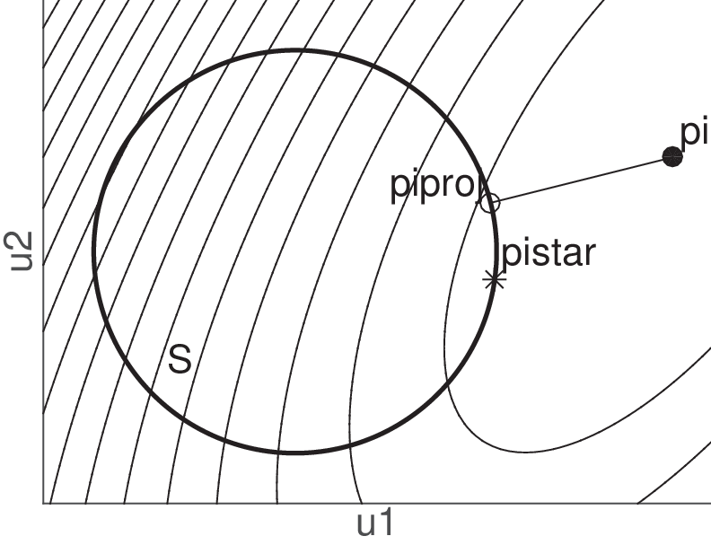
Consider the projection (12) of the policy (3) obtained via QQ-learning. We ought to first observe that if Q𝜽=Q⋆Q_{\boldsymbol{\mathrm{\theta}}}=Q_{\star} holds over 𝕎\mathbb{W}, the projected policy is optimal whenever the learned policy 𝝅𝜽∈𝕊⁡(𝐱){\boldsymbol{\mathrm{\pi}}}_{\boldsymbol{\mathrm{\theta}}}\in\mathbb{S}\left(\boldsymbol{\mathrm{x}}\right). Unfortunately, this observation does not necessarily extend to the situation where 𝝅𝜽​(𝐱)∉𝕊​(𝐱){\boldsymbol{\mathrm{\pi}}}_{\boldsymbol{\mathrm{\theta}}}\left(\boldsymbol{\mathrm{x}}\right)\notin\mathbb{S}\left(\boldsymbol{\mathrm{x}}\right). In order to support this observation, let us consider a trivial example displayed in Fig. 1. This shows that 𝝅𝜽⟂​(𝐱)=𝝅⋆safe​(𝐱){\boldsymbol{\mathrm{\pi}}}_{\boldsymbol{\mathrm{\theta}}}^{\perp}\left(\boldsymbol{\mathrm{x}}\right)=\boldsymbol{\mathrm{\pi}}_{\star}^{\mathrm{safe}}\left(\boldsymbol{\mathrm{x}}\right) does not hold in general.

Refer to caption
Figure 1: Illustration of the possible loss of optimality resulting from using the projection (12) in QQ-learning.

However, Lemma 1 readily delivers a way to alleviate this problem: assuming that a QQ-function approximation Q𝜽≈Q⋆Q_{\boldsymbol{\mathrm{\theta}}}\approx Q_{\star} over ℤ\mathbb{Z} has been learned, a safe policy can be devised from using 𝝅⋆safe​(𝐱)\boldsymbol{\mathrm{\pi}}_{\star}^{\mathrm{safe}}\left(\boldsymbol{\mathrm{x}}\right) obtained from (14) as opposed to a generic projection (12). One then must be careful to include the input restriction 𝐮∈𝕊⁡(𝐱)\boldsymbol{\mathrm{u}}\in\mathbb{S}\left(\boldsymbol{\mathrm{x}}\right) in the evaluation of the TD error underlying the QQ-learning. When using SARSA, no special care needs to be taken in the learning process, as (14) generates all inputs in 𝕊⁡(𝐱)\mathbb{S}\left(\boldsymbol{\mathrm{x}}\right). An approach to formulate (14) via robust MPC is presented in (Zanon and Gros 2019).

This section shows that the direct minimization (14) of the QQ function approximation under the safety constraints is arguably better suited than the two steps approach: (3) followed by (12). We ought to extend the discussion to the context of the policy gradient methods using actor-critic techniques. This discussion is more technical, and is the object of the next section.

4 Safe policy gradient via projection

Policy gradient methods are often preferred over QQ-learning because they alleviate the known issue that solving the least-squares problem (13) does not necessarily imply that one has found parameter 𝜽\boldsymbol{\mathrm{\theta}} that yields the best closed-loop performance of the policy (3). Indeed, policy gradient methods seek a direct minimization of the closed-loop cost (1) via gradient steps over (1), and therefore yield (at least locally) optimal policy parameters. Similarly to the discussion of Section 3, when deploying policy gradient techniques jointly with a projection on the safe set (12), the optimality of the resulting policy is unclear. As a matter of fact, we will show in this section that the learning process ought to be corrected in order for the estimation of the gradient of (1) to be unbiased. Subsection 4.1 will cover the deterministic policy gradient case, while subsection 4.2 will cover the stochastic policy gradient case.

4.1 Projected Policy and Deterministic Policy Gradient

In the context of deterministic policies, we will show next that a correction must be applied in the policy gradient computation to account for the safe projection (12). This correction is provided in the following Proposition.

Proposition 1

Consider the projection (12) where ∥⋅∥\|\cdot\| stands for the Euclidian norm, and assume that the constraints (12b) satisfy the Linear Constraint Qualification (LICQ) and strict Second-Order Sufficient Conditions (SOSC). The gradient of the projected policy 𝛑𝛉⟂{\boldsymbol{\mathrm{\pi}}}_{\boldsymbol{\mathrm{\theta}}}^{\perp} with respect to the policy parameters 𝛉\boldsymbol{\mathrm{\theta}} then reads as:

∇𝜽𝝅𝜽⟂​(𝐱)\displaystyle\nabla_{\boldsymbol{\mathrm{\theta}}}{\boldsymbol{\mathrm{\pi}}}_{\boldsymbol{\mathrm{\theta}}}^{\perp}\left(\boldsymbol{\mathrm{x}}\right) =∇𝜽𝝅𝜽​(𝐱)​M​(𝐱),\displaystyle=\nabla_{\boldsymbol{\mathrm{\theta}}}{\boldsymbol{\mathrm{\pi}}}_{\boldsymbol{\mathrm{\theta}}}\left(\boldsymbol{\mathrm{x}}\right)M\left(\boldsymbol{\mathrm{x}}\right), (17a)
M⁡(𝐱)\displaystyle M\left(\boldsymbol{\mathrm{x}}\right) =𝒩​(𝒩⊤​H​𝒩)−1​𝒩⊤,\displaystyle=\mathcal{N}\left(\mathcal{N}^{\top}H\mathcal{N}\right)^{-1}\mathcal{N}^{\top}, (17b)

where 𝒩∈ℝm×n𝔸\mathcal{N}\in\mathbb{R}^{m\times n_{\mathbb{A}}} is a state-dependent orthonormal null space to the gradient of the strictly active constraints, i.e.:

∇𝐮𝐬𝔸​(𝐱,𝝅𝜽⟂​(𝐱))⊤​𝒩​(𝐱)=0,𝒩​(𝐱)⊤​𝒩​(𝐱)=I,\displaystyle\nabla_{\boldsymbol{\mathrm{u}}}\boldsymbol{\mathrm{s}}_{\mathbb{A}}\left(\boldsymbol{\mathrm{x}},{\boldsymbol{\mathrm{\pi}}}_{\boldsymbol{\mathrm{\theta}}}^{\perp}\left(\boldsymbol{\mathrm{x}}\right)\right)^{\top}\mathcal{N}\left(\boldsymbol{\mathrm{x}}\right)=0,\quad\mathcal{N}\left(\boldsymbol{\mathrm{x}}\right)^{\top}\mathcal{N}\left(\boldsymbol{\mathrm{x}}\right)=I, (18)

with 𝔸\mathbb{A} gathering the set of strictly active constraints 𝐬\boldsymbol{\mathrm{s}}, and HH is the Hessian associated to (12).

{pf}

The solution to (12) satisfies the KKT conditions:

𝐫=[∇𝐮ℒ​(𝐱,𝐮,𝝁)diag⁡(𝝁𝔸)​𝐬𝔸​(𝐱,𝐮)]\displaystyle\boldsymbol{\mathrm{r}}=\left[\begin{array}[]{c}\nabla_{\boldsymbol{\mathrm{u}}}\mathcal{L}\left(\boldsymbol{\mathrm{x}},\boldsymbol{\mathrm{u}},\boldsymbol{\mathrm{\mu}}\right)\\ \mathrm{diag}(\boldsymbol{\mathrm{\mu}}_{\mathbb{A}})\boldsymbol{\mathrm{s}}_{\mathbb{A}}\left(\boldsymbol{\mathrm{x}},\boldsymbol{\mathrm{u}}\right)\end{array}\right] =0,\displaystyle=0,

where ℒ=12​‖𝐮−𝝅𝜽​(𝐱)‖2+𝝁⊤​𝐬​(𝐱,𝐮)\mathcal{L}=\frac{1}{2}\|\boldsymbol{\mathrm{u}}-{\boldsymbol{\mathrm{\pi}}}_{\boldsymbol{\mathrm{\theta}}}\left(\boldsymbol{\mathrm{x}}\right)\|^{2}+\boldsymbol{\mathrm{\mu}}^{\top}\boldsymbol{\mathrm{s}}\left(\boldsymbol{\mathrm{x}},\boldsymbol{\mathrm{u}}\right). The Implicit Function Theorem guarantees that if LICQ and SOSC hold, the gradient of the projected policy reads as:

[H∇𝐮𝐬𝔸∇𝐮𝐬𝔸⊤𝟘]​[∂𝐮/∂𝜽∂𝝁𝔸/∂𝜽]=−[∇𝐮​𝜽ℒ⊤𝟎].\displaystyle\left[\begin{array}[]{cc}H&\nabla_{\boldsymbol{\mathrm{u}}}\boldsymbol{\mathrm{s}}_{\mathbb{A}}\\ \nabla_{\boldsymbol{\mathrm{u}}}\boldsymbol{\mathrm{s}}_{\mathbb{A}}^{\top}&\mathbb{0}\end{array}\right]\left[\begin{array}[]{c}\partial\boldsymbol{\mathrm{u}}/\partial\boldsymbol{\mathrm{\theta}}\\ \partial\boldsymbol{\mathrm{\mu}}_{\mathbb{A}}/\partial\boldsymbol{\mathrm{\theta}}\end{array}\right]=-\left[\begin{array}[]{c}\nabla_{\boldsymbol{\mathrm{u}}\boldsymbol{\mathrm{\theta}}}\mathcal{L}^{\top}\\ \boldsymbol{\mathrm{0}}\end{array}\right].

We then observe that ∇𝐮𝐬𝔸⊤​∂𝐮/∂𝜽=0\nabla_{\boldsymbol{\mathrm{u}}}\boldsymbol{\mathrm{s}}_{\mathbb{A}}^{\top}\partial\boldsymbol{\mathrm{u}}/\partial\boldsymbol{\mathrm{\theta}}=0 entails that

∇𝜽𝝅𝜽⟂​(𝐱)⊤=∂𝐮∂𝜽=𝒩​𝐧,\displaystyle\nabla_{\boldsymbol{\mathrm{\theta}}}{\boldsymbol{\mathrm{\pi}}}_{\boldsymbol{\mathrm{\theta}}}^{\perp}\left(\boldsymbol{\mathrm{x}}\right)^{\top}=\frac{\partial\boldsymbol{\mathrm{u}}}{\partial\boldsymbol{\mathrm{\theta}}}=\mathcal{N}\boldsymbol{\mathrm{n}}, (27)

for some vector 𝐧\boldsymbol{\mathrm{n}}. We further observe that:

𝒩⊤​(H​∂𝐮∂𝜽+∇𝐮𝐬𝔸​∂𝝁𝔸∂𝜽)\displaystyle\mathcal{N}^{\top}\left(H\frac{\partial\boldsymbol{\mathrm{u}}}{\partial\boldsymbol{\mathrm{\theta}}}+\nabla_{\boldsymbol{\mathrm{u}}}\boldsymbol{\mathrm{s}}_{\mathbb{A}}\frac{\partial\boldsymbol{\mathrm{\mu}}_{\mathbb{A}}}{\partial\boldsymbol{\mathrm{\theta}}}\right) =−𝒩⊤​∇𝐮​𝜽ℒ⊤\displaystyle=-\mathcal{N}^{\top}\nabla_{\boldsymbol{\mathrm{u}}\boldsymbol{\mathrm{\theta}}}\mathcal{L}^{\top}

follows from (4.1), such that, using (18) and (27) we get

𝒩⊤​H​𝒩​𝐧\displaystyle\mathcal{N}^{\top}H\mathcal{N}\boldsymbol{\mathrm{n}} =−𝒩⊤​∇𝐮​𝜽ℒ⊤.\displaystyle=-\mathcal{N}^{\top}\nabla_{\boldsymbol{\mathrm{u}}\boldsymbol{\mathrm{\theta}}}\mathcal{L}^{\top}. (28)

Since we have

∇𝐮​𝜽ℒ=−∇𝜽𝝅𝜽,H=𝕀+∇𝐮2(𝝁𝔸⊤​𝐬𝔸),\displaystyle\nabla_{\boldsymbol{\mathrm{u}}\boldsymbol{\mathrm{\theta}}}\mathcal{L}=-\nabla_{\boldsymbol{\mathrm{\theta}}}{\boldsymbol{\mathrm{\pi}}}_{\boldsymbol{\mathrm{\theta}}},\quad H=\mathbb{I}+\nabla^{2}_{\boldsymbol{\mathrm{u}}}\left(\boldsymbol{\mathrm{\mu}}_{\mathbb{A}}^{\top}\boldsymbol{\mathrm{s}}_{\mathbb{A}}\right), (29)

this entails 𝐧=(𝒩⊤​H​𝒩)−1​𝒩⊤​∇𝜽𝝅𝜽⊤\boldsymbol{\mathrm{n}}=(\mathcal{N}^{\top}H\mathcal{N})^{-1}\mathcal{N}^{\top}\nabla_{\boldsymbol{\mathrm{\theta}}}{\boldsymbol{\mathrm{\pi}}}_{\boldsymbol{\mathrm{\theta}}}^{\top}.

■\blacksquare Hence the gradient of the projected policy is a form of projection of the gradient of the original policy 𝝅𝜽​(𝐱){\boldsymbol{\mathrm{\pi}}}_{\boldsymbol{\mathrm{\theta}}}\left(\boldsymbol{\mathrm{x}}\right) into the null-space of the safety constraints. We will define 𝒩⁡(𝐱)=Im×m\mathcal{N}\left(\boldsymbol{\mathrm{x}}\right)=I_{m\times m} for all 𝐱\boldsymbol{\mathrm{x}} for which all constraints are strictly inactive, and 𝒩⁡(𝐱)=0m×1\mathcal{N}\left(\boldsymbol{\mathrm{x}}\right)=0_{{m\times 1}} for all 𝐱\boldsymbol{\mathrm{x}} where the active constraints fully block the inputs. We observe that the set of states 𝐱\boldsymbol{\mathrm{x}} where some constraints are weakly active—such that the gradient of the policy is only defined in the sense of its sub-gradients—is of zero measure and can therefore be disregarded in the context discussed here. In the particular case of a safety set 𝕊\mathbb{S} described as a polytope, such that the constraints 𝐬\boldsymbol{\mathrm{s}} are affine, H=𝕀H=\mathbb{I} holds and matrix MM simplifies to M=𝒩​𝒩⊤M=\mathcal{N}\mathcal{N}^{\top}.

We can then form the Corollary to Proposition 1 providing a correct policy gradient evaluation.

Corollary 1

Let us assume that (12) fulfills LICQ and SOSC. Then the policy gradient associated to the safe policy 𝛑𝛉⟂{\boldsymbol{\mathrm{\pi}}}^{\perp}_{\boldsymbol{\mathrm{\theta}}} reads as:

∇𝜽J​(𝝅𝜽⟂)\displaystyle\nabla_{\boldsymbol{\mathrm{\theta}}}J\left({\boldsymbol{\mathrm{\pi}}}^{\perp}_{\boldsymbol{\mathrm{\theta}}}\right) =𝔼⁡[∇𝜽𝝅𝜽⟂​∇𝐮A𝝅𝜽⟂]\displaystyle=\mathbb{E}\left[\nabla_{\boldsymbol{\mathrm{\theta}}}{\boldsymbol{\mathrm{\pi}}}_{\boldsymbol{\mathrm{\theta}}}^{\perp}\nabla_{\boldsymbol{\mathrm{u}}}A_{\boldsymbol{\mathrm{\pi}}^{\perp}_{\boldsymbol{\mathrm{\theta}}}}\right] (30)
=𝔼⁡[∇𝜽𝝅𝜽​M​∇𝐮A𝝅𝜽⟂]\displaystyle\quad=\mathbb{E}\left[\nabla_{\boldsymbol{\mathrm{\theta}}}{\boldsymbol{\mathrm{\pi}}}_{\boldsymbol{\mathrm{\theta}}}M\nabla_{\boldsymbol{\mathrm{u}}}A_{\boldsymbol{\mathrm{\pi}}^{\perp}_{\boldsymbol{\mathrm{\theta}}}}\right]

where A𝛑𝛉⟂A_{{\boldsymbol{\mathrm{\pi}}}^{\perp}_{\boldsymbol{\mathrm{\theta}}}} is the advantage function associated to the projected policy 𝛑𝛉⟂{\boldsymbol{\mathrm{\pi}}}^{\perp}_{\boldsymbol{\mathrm{\theta}}}. All terms in (30) are evaluated at 𝐱,\boldsymbol{\mathrm{x}}, 𝐮=𝛑𝛉⟂​(𝐱)\boldsymbol{\mathrm{u}}={\boldsymbol{\mathrm{\pi}}}^{\perp}_{\boldsymbol{\mathrm{\theta}}}\left(\boldsymbol{\mathrm{x}}\right) with 𝐱\boldsymbol{\mathrm{x}} distributed according to the probability density of the states in closed-loop under policy 𝛑𝛉⟂{\boldsymbol{\mathrm{\pi}}}^{\perp}_{\boldsymbol{\mathrm{\theta}}}.

{pf}

We observe that for any 𝐱\boldsymbol{\mathrm{x}} such that no constraint is weakly active, the equality

∇𝜽𝝅𝜽⟂​∇𝐮A𝝅𝜽⟂=∇𝜽𝝅𝜽​M​∇𝐮A𝝅𝜽⟂\displaystyle\nabla_{\boldsymbol{\mathrm{\theta}}}{\boldsymbol{\mathrm{\pi}}}_{\boldsymbol{\mathrm{\theta}}}^{\perp}\nabla_{\boldsymbol{\mathrm{u}}}A_{{\boldsymbol{\mathrm{\pi}}}^{\perp}_{\boldsymbol{\mathrm{\theta}}}}=\nabla_{\boldsymbol{\mathrm{\theta}}}{\boldsymbol{\mathrm{\pi}}}_{\boldsymbol{\mathrm{\theta}}}M\nabla_{\boldsymbol{\mathrm{u}}}A_{{\boldsymbol{\mathrm{\pi}}}^{\perp}_{\boldsymbol{\mathrm{\theta}}}}

holds. If (12) fulfills the LICQ condition, the set of states where some constraints are weakly active is of zero-measure, such that the equality

∇𝜽J​(𝝅𝜽⟂)\displaystyle\nabla_{\boldsymbol{\mathrm{\theta}}}J\left({\boldsymbol{\mathrm{\pi}}}^{\perp}_{\boldsymbol{\mathrm{\theta}}}\right) =𝔼⁡[∇𝜽𝝅𝜽⟂​∇𝐮A𝝅𝜽⟂]=𝔼⁡[∇𝜽𝝅𝜽​M​∇𝐮A𝝅𝜽⟂]\displaystyle=\mathbb{E}\left[\nabla_{\boldsymbol{\mathrm{\theta}}}{\boldsymbol{\mathrm{\pi}}}_{\boldsymbol{\mathrm{\theta}}}^{\perp}\nabla_{\boldsymbol{\mathrm{u}}}A_{{\boldsymbol{\mathrm{\pi}}}^{\perp}_{\boldsymbol{\mathrm{\theta}}}}\right]=\mathbb{E}\left[\nabla_{\boldsymbol{\mathrm{\theta}}}{\boldsymbol{\mathrm{\pi}}}_{\boldsymbol{\mathrm{\theta}}}M\nabla_{\boldsymbol{\mathrm{u}}}A_{{\boldsymbol{\mathrm{\pi}}}^{\perp}_{\boldsymbol{\mathrm{\theta}}}}\right]

holds.

■\blacksquare

If deploying the projected policy approach (12) and an actor-critic method not accounting for the projection operation, the policy gradient will generally be such that:

∇𝜽J​(𝝅𝜽⟂)≠𝔼⁡[∇𝜽𝝅𝜽​∇𝐮A𝝅𝜽⟂],\displaystyle{\nabla_{\boldsymbol{\mathrm{\theta}}}J}\left({\boldsymbol{\mathrm{\pi}}}^{\perp}_{\boldsymbol{\mathrm{\theta}}}\right)\neq\mathbb{E}\left[\nabla_{\boldsymbol{\mathrm{\theta}}}{\boldsymbol{\mathrm{\pi}}}_{\boldsymbol{\mathrm{\theta}}}\nabla_{\boldsymbol{\mathrm{u}}}A_{{\boldsymbol{\mathrm{\pi}}}^{\perp}_{\boldsymbol{\mathrm{\theta}}}}\right], (31)

where the projection matrix M⁡(𝐱)M\left(\boldsymbol{\mathrm{x}}\right) is omitted. This omission will, in general, produce a biased policy gradient (31) if the policy projection is not accounted for in the RL method when computing the policy gradient. It is therefore recommended to form and use the projection matrix MM when computing the policy gradient.

It can be advantageous in some cases to adopt a stochastic policy gradient method instead of the deterministic one discussed in this section. In the stochastic policy gradient, the same question arises regarding the learning process being biased by the projection in the safe set. We discuss this case in the next subsection.

4.2 Projected Policy and Stochastic Policy Gradient

When using a stochastic policy gradient technique, the inputs are chosen as samples 𝐮s\boldsymbol{\mathrm{u}}_{\mathrm{s}} drawn from a parametrized conditional probability density representing the policy:

𝐮s∼π𝜽[⋅|𝐱].\displaystyle\boldsymbol{\mathrm{u}}_{\mathrm{s}}\sim\pi_{\boldsymbol{\mathrm{\theta}}}[\,\cdot\,|\,\boldsymbol{\mathrm{x}}\,]. (32)

The safe projection then ought to be performed over the samples 𝐮s\boldsymbol{\mathrm{u}}_{\mathrm{s}}, i.e.:

𝝅𝜽⟂​(𝐱,𝐮s)=arg​min𝐮\displaystyle\boldsymbol{\mathrm{\pi}}^{\perp}_{\boldsymbol{\mathrm{\theta}}}\left(\boldsymbol{\mathrm{x}},\boldsymbol{\mathrm{u}}_{\mathrm{s}}\right)=\mathrm{arg}\min_{\boldsymbol{\mathrm{u}}} 12​‖𝐮−𝐮s‖2\displaystyle\quad\frac{1}{2}\|\boldsymbol{\mathrm{u}}-\boldsymbol{\mathrm{u}}_{\mathrm{s}}\|^{2}\ (33a)
s.t.\displaystyle\mathrm{s.t.} 𝐬⁡(𝐱,𝐮)≤0.\displaystyle\quad\boldsymbol{\mathrm{s}}\left(\boldsymbol{\mathrm{x}},\boldsymbol{\mathrm{u}}\right)\leq 0. (33b)

The inputs generated by 𝝅𝜽⟂​(𝐱,𝐮s)\boldsymbol{\mathrm{\pi}}_{\boldsymbol{\mathrm{\theta}}}^{\perp}\left(\boldsymbol{\mathrm{x}},\boldsymbol{\mathrm{u}}_{\mathrm{s}}\right) are safe by construction. The resulting projected policy is itself stochastic, as it results from the nonlinear transformation (33) of the probability density π𝜽[⋅|𝐱]\pi_{\boldsymbol{\mathrm{\theta}}}[\,\cdot\,|\,\boldsymbol{\mathrm{x}}\,]. Let us label the probability density resulting from the projection of the stochastic policy π𝜽[⋅|𝐱]\pi_{\boldsymbol{\mathrm{\theta}}}[\,\cdot\,|\,\boldsymbol{\mathrm{x}}\,] via (33) as π𝜽⟂[⋅|𝐱]\pi_{\boldsymbol{\mathrm{\theta}}}^{\perp}[\,\cdot\,|\,\boldsymbol{\mathrm{x}}\,]. Unfortunately, since the projection operator defined by (33) is not injective, the density π𝜽⟂[⋅|𝐱]\pi^{\perp}_{\boldsymbol{\mathrm{\theta}}}[\,\cdot\,|\,\boldsymbol{\mathrm{x}}\,] can adopt a “Dirac-like” structure on the boundary ∂𝕊\partial\mathbb{S} of the safe set 𝕊\mathbb{S}, due to the fact that sets of inputs of dimension larger than one is projected onto a single point on ∂𝕊\partial\mathbb{S}. This issue is illustrated in Fig. 2.

Refer to caption
Figure 2: Illustration of the Dirac-like effect resulting from projecting a Normally distributed stochastic policy on a safe set, chosen as a circle here.

As a result, the score function of π𝜽⟂\pi^{\perp}_{\boldsymbol{\mathrm{\theta}}} is not trivially defined, and the construction of the policy gradient of π𝜽⟂\pi^{\perp}_{\boldsymbol{\mathrm{\theta}}} is not obvious. The following proposition shows that a trivial modification of the stochastic policy gradient allows one to circumvent this difficulty.

Proposition 2

The policy gradient associated to π𝛉⟂\pi^{\perp}_{\boldsymbol{\mathrm{\theta}}} is given by the actor-critic equation:

∇𝜽J​(π𝜽⟂)=𝔼⁡[∇𝜽​log​π𝜽​[𝐮s|𝐱]​Aπ𝜽⟂​(𝐱,𝐮)],\displaystyle{\nabla_{\boldsymbol{\mathrm{\theta}}}J}\left(\pi^{\perp}_{\boldsymbol{\mathrm{\theta}}}\right)=\mathbb{E}\left[\nabla_{\boldsymbol{\mathrm{\theta}}}\log\pi_{\boldsymbol{\mathrm{\theta}}}[\boldsymbol{\mathrm{u}}_{\mathrm{s}}|\boldsymbol{\mathrm{x}}]A_{\pi^{\perp}_{\boldsymbol{\mathrm{\theta}}}}(\boldsymbol{\mathrm{x}},\boldsymbol{\mathrm{u}})\right], (34)

where 𝐮=𝛑𝛉⟂​(𝐱,𝐮s)\boldsymbol{\mathrm{u}}=\boldsymbol{\mathrm{\pi}}_{\boldsymbol{\mathrm{\theta}}}^{\perp}\left(\boldsymbol{\mathrm{x}},\boldsymbol{\mathrm{u}}_{\mathrm{s}}\right) is the input obtained from (33) satisfying LICQ and SOSC, and the expected value operator 𝔼⁡[⋅]\mathbb{E}[\cdot] is taken over the state and input distribution obtained in closed-loop under the projected stochastic policy π𝛉⟂[⋅|𝐱]\pi^{\perp}_{\boldsymbol{\mathrm{\theta}}}[\,\cdot\,|\,\boldsymbol{\mathrm{x}}\,].

{pf}

In order to build a proof using simple arguments, let us consider the interior-point approximation of the projection problem (33):

𝝅τ​(𝐱,𝐮s)=arg​min𝐮​12​‖𝐮−𝐮s‖2−τ​∑ilog⁡(−𝐡i​(𝐱,𝐮)),\displaystyle\hskip-6.0pt\boldsymbol{\mathrm{\pi}}_{\tau}\hskip-1.0pt\left(\boldsymbol{\mathrm{x}},\boldsymbol{\mathrm{u}}_{\mathrm{s}}\right)\hskip-1.0pt=\hskip-1.0pt\mathrm{arg}\min_{\boldsymbol{\mathrm{u}}}\frac{1}{2}\|\boldsymbol{\mathrm{u}}-\boldsymbol{\mathrm{u}}_{\mathrm{s}}\|^{2}\hskip-1.0pt-\hskip-1.0pt\tau{\sum}_{i}\log\hskip-1.0pt\left(-\boldsymbol{\mathrm{h}}_{i}\hskip-1.0pt\left(\boldsymbol{\mathrm{x}},\boldsymbol{\mathrm{u}}\right)\right),\hskip-2.0pt (35)

such that ‖𝝅τ​(𝐱,𝐮s)−𝝅𝜽⟂​(𝐱,𝐮s)‖=O⁡(τ)\left\|\boldsymbol{\mathrm{\pi}}_{\tau}\left(\boldsymbol{\mathrm{x}},\boldsymbol{\mathrm{u}}_{\mathrm{s}}\right)-\boldsymbol{\mathrm{\pi}}^{\perp}_{\boldsymbol{\mathrm{\theta}}}\left(\boldsymbol{\mathrm{x}},\boldsymbol{\mathrm{u}}_{\mathrm{s}}\right)\right\|=O(\tau) holds. Let us define πτ[⋅|𝐱]\pi^{\tau}[\,\cdot\,|\,\boldsymbol{\mathrm{x}}\,] the density resulting from transforming π𝜽[⋅|𝐱]\pi_{\boldsymbol{\mathrm{\theta}}}[\,\cdot\,|\,\boldsymbol{\mathrm{x}}\,] via (35). If (33) satisfying LICQ and SOSC, then (35) is locally bijective in 𝐮s\boldsymbol{\mathrm{u}}_{\mathrm{s}}, and the score function associated to πτ\pi^{\tau} is well-defined. The associated policy gradient reads as:

∇𝜽J​(πτ)=𝔼⁡[∇𝜽​log​πτ​[𝐮|𝐱]​Aπτ​(𝐱,𝐮)],\displaystyle{\nabla_{\boldsymbol{\mathrm{\theta}}}J}\left(\pi^{\tau}\right)=\mathbb{E}\left[\nabla_{\boldsymbol{\mathrm{\theta}}}\log\pi^{\tau}[\boldsymbol{\mathrm{u}}|\boldsymbol{\mathrm{x}}]A_{\pi^{\tau}}(\boldsymbol{\mathrm{x}},\boldsymbol{\mathrm{u}})\right], (36)

where 𝐮=𝝅τ​(𝐱,𝐮s)\boldsymbol{\mathrm{u}}=\boldsymbol{\mathrm{\pi}}_{\tau}\left(\boldsymbol{\mathrm{x}},\boldsymbol{\mathrm{u}}_{\mathrm{s}}\right). Let us further define function 𝝅τ−1\boldsymbol{\mathrm{\pi}}_{\tau}^{-1} the local inverse of 𝝅τ\boldsymbol{\mathrm{\pi}}^{\tau} at 𝐮s\boldsymbol{\mathrm{u}}_{\mathrm{s}}, i.e.,

𝝅τ−1​(𝐱,𝝅τ​(𝐱,𝐮))=𝐮,\displaystyle\boldsymbol{\mathrm{\pi}}_{\tau}^{-1}\left(\boldsymbol{\mathrm{x}},\boldsymbol{\mathrm{\pi}}_{\tau}\left(\boldsymbol{\mathrm{x}},\boldsymbol{\mathrm{u}}\right)\right)=\boldsymbol{\mathrm{u}}, (37)

holds in a neighborhood of 𝐮s\boldsymbol{\mathrm{u}}_{\mathrm{s}}. The existence of (37) is guaranteed for τ>0\tau>0 if (33) satisfies LICQ and SOSC. We then observe that the transformation (35) of the density π𝜽\pi_{\boldsymbol{\mathrm{\theta}}} yields:

πτ​[𝐮|𝐱]\displaystyle\pi^{\tau}\left[\boldsymbol{\mathrm{u}}\,|\,\boldsymbol{\mathrm{x}}\right] =π⁡[𝝅τ−1​(𝐱,𝐮)|𝐱]​det(∂𝝅τ−1​(𝐱,𝐮)∂𝐮).\displaystyle=\pi\left[\,\boldsymbol{\mathrm{\pi}}_{\tau}^{-1}\left(\boldsymbol{\mathrm{x}},\boldsymbol{\mathrm{u}}\right)\,|\,\boldsymbol{\mathrm{x}}\,\right]\det\left(\frac{\partial\boldsymbol{\mathrm{\pi}}_{\tau}^{-1}\left(\boldsymbol{\mathrm{x}},\boldsymbol{\mathrm{u}}\right)}{\partial\boldsymbol{\mathrm{u}}}\right). (38)

For 𝐮s\boldsymbol{\mathrm{u}}_{\mathrm{s}} given, (35) is independent of 𝜽\boldsymbol{\mathrm{\theta}}, such that

∇𝜽det(∂𝝅τ−1​(𝐱,𝐮)∂𝐮)=0.\displaystyle\nabla_{\boldsymbol{\mathrm{\theta}}}\det\left(\frac{\partial\boldsymbol{\mathrm{\pi}}_{\tau}^{-1}\left(\boldsymbol{\mathrm{x}},\boldsymbol{\mathrm{u}}\right)}{\partial\boldsymbol{\mathrm{u}}}\right)=0. (39)

As a result, the score function of πτ\pi^{\tau} reads as:

∇𝜽​log​πτ​[𝐮|𝐱]\displaystyle\nabla_{\boldsymbol{\mathrm{\theta}}}\log\pi^{\tau}\left[\boldsymbol{\mathrm{u}}\,|\,\boldsymbol{\mathrm{x}}\right] =∇𝜽​log​π𝜽​[𝝅τ−1​(𝐱,𝐮)|𝐱]\displaystyle=\nabla_{\boldsymbol{\mathrm{\theta}}}\log\pi_{\boldsymbol{\mathrm{\theta}}}\left[\,\boldsymbol{\mathrm{\pi}}_{\tau}^{-1}\left(\boldsymbol{\mathrm{x}},\boldsymbol{\mathrm{u}}\right)\,|\,\boldsymbol{\mathrm{x}}\,\right]
=∇𝜽​log​π𝜽​[𝐮s|𝐱],\displaystyle=\nabla_{\boldsymbol{\mathrm{\theta}}}\log\pi_{\boldsymbol{\mathrm{\theta}}}\left[\,\boldsymbol{\mathrm{u}}_{\mathrm{s}}\,|\,\boldsymbol{\mathrm{x}}\,\right], (40)

where 𝐮s\boldsymbol{\mathrm{u}}_{\mathrm{s}} is the sample corresponding to 𝐮\boldsymbol{\mathrm{u}} obtained from (35). Combining (4.2) and (36), we observe that

∇𝜽J​(πτ)=𝔼⁡[∇𝜽​log​π𝜽​[𝐮s|𝐱]​Aπτ​(𝐱,𝝅τ​(𝐱,𝐮s))].\displaystyle{\nabla_{\boldsymbol{\mathrm{\theta}}}J}\left(\pi^{\tau}\right)=\mathbb{E}\left[\nabla_{\boldsymbol{\mathrm{\theta}}}\log\pi_{\boldsymbol{\mathrm{\theta}}}\left[\,\boldsymbol{\mathrm{u}}_{\mathrm{s}}\,|\,\boldsymbol{\mathrm{x}}\,\right]A_{\pi^{\tau}}(\boldsymbol{\mathrm{x}},\boldsymbol{\mathrm{\pi}}_{\tau}\left(\boldsymbol{\mathrm{x}},\boldsymbol{\mathrm{u}}_{\mathrm{s}}\right))\right].

The equivalence between (35) and (33) for τ→0\tau\rightarrow 0 implies that (34) holds.

■\blacksquare

Remark 2

Proposition 2 allows one to use the projection technique in the context of RL based on a stochastic policy approach together with an actor-critic technique, where the score function of the unprojected policy can be used in conjunction with the advantage function associated to the projected policy. The score function of the unprojected policy must then be evaluated on the unprojected sample, rather than on the projected input applied to the system.

As mentioned earlier, the construction of the constraints 𝐬\boldsymbol{\mathrm{s}} underlying the safe set 𝕊⁡(𝐱)\mathbb{S}\left(\boldsymbol{\mathrm{x}}\right) can be difficult. We extend next the proposed results to MPC-based techniques allowing one to build the safety constraints implicitly, via model predictive control techniques.

5 MPC-based projections

It is in general difficult to build the safe set 𝕊\mathbb{S} from condition (9). Indeed, an input 𝐮\boldsymbol{\mathrm{u}} applied at a given time kk can have lasting consequences and, while not endangering the system at time kk, jeopardize its safety in the future. In order to alleviate this problem, the safety constraints can be built implicitly via Model Predictive Control (MPC) techniques. In that context, let us consider

𝐗k​(𝐱,𝐮0,𝝅𝕊),k=0,…,∞\displaystyle\boldsymbol{\mathrm{X}}_{k}\left(\boldsymbol{\mathrm{x}},\boldsymbol{\mathrm{u}}_{0},\boldsymbol{\mathrm{\pi}}^{\mathbb{S}}\right),\quad k=0,\ldots,\infty (41)

an outer approximation of the trajectory dispersion of the real system starting from the initial conditions 𝐱\boldsymbol{\mathrm{x}}, hence 𝐗0​(𝐱,𝐮0,𝝅𝕊)=𝐱\boldsymbol{\mathrm{X}}_{0}\left(\boldsymbol{\mathrm{x}},\boldsymbol{\mathrm{u}}_{0},\boldsymbol{\mathrm{\pi}}^{\mathbb{S}}\right)=\boldsymbol{\mathrm{x}}, and subject to the input sequence 𝐮0,𝐮k=𝝅𝕊​(𝐱k)\boldsymbol{\mathrm{u}}_{0},\,\boldsymbol{\mathrm{u}}_{k}=\boldsymbol{\mathrm{\pi}}^{\mathbb{S}}\left(\boldsymbol{\mathrm{x}}_{k}\right), where 𝝅𝕊\boldsymbol{\mathrm{\pi}}^{\mathbb{S}} is an arbitrary policy. The safe set can then be described as an inner approximation:

𝕊⁡(𝐱)\displaystyle\mathbb{S}\left(\boldsymbol{\mathrm{x}}\right) ⊆{𝐮0|∃𝝅𝕊s.t.𝐡(𝐱k,𝝅𝕊(𝐱k))≤0\displaystyle\subseteq\left\{\,\boldsymbol{\mathrm{u}}_{0}\,\,\,|\,\,\,\exists\,\boldsymbol{\mathrm{\pi}}^{\mathbb{S}}\quad\mathrm{s.t.}\quad\boldsymbol{\mathrm{h}}\left(\boldsymbol{\mathrm{x}}_{k},\boldsymbol{\mathrm{\pi}}^{\mathbb{S}}(\boldsymbol{\mathrm{x}}_{k})\right)\leq 0\right.
∀𝐱k∈𝐗k(𝐱,𝐮0,𝝅𝕊),∀k>0},\displaystyle\hskip 50.00008pt\left.\forall\,\boldsymbol{\mathrm{x}}_{k}\in\boldsymbol{\mathrm{X}}_{k}\left(\boldsymbol{\mathrm{x}},\boldsymbol{\mathrm{u}}_{0},\boldsymbol{\mathrm{\pi}}^{\mathbb{S}}\right),\quad\forall\,k>0\right\}, (42)

which can then be used in (12) or (33). If MPC techniques are used, a generalization of the projection technique can be considered. In the deterministic policy case, one can then use the generic robust formulation:

(𝐮0,𝝅𝕊)​(𝐱0)=arg⁡min𝐮0,𝝅𝕊\displaystyle\hskip-4.0pt\left(\boldsymbol{\mathrm{u}}_{0},\boldsymbol{\mathrm{\pi}}^{\mathbb{S}}\right)\hskip-2.0pt\left(\boldsymbol{\mathrm{x}}_{0}\right)\hskip-1.0pt=\arg\min_{\boldsymbol{\mathrm{u}}_{0},\boldsymbol{\mathrm{\pi}}^{\mathbb{S}}} 12​‖𝐮0−𝝅𝜽​(𝐱0)‖2+ϕ⁡(𝝅𝕊,𝝅𝜽)\displaystyle\,\frac{1}{2}\|\boldsymbol{\mathrm{u}}_{0}\hskip-1.0pt-\hskip-1.0pt\boldsymbol{\mathrm{\pi}}_{\boldsymbol{\mathrm{\theta}}}\hskip-1.0pt\left(\boldsymbol{\mathrm{x}}_{0}\right)\hskip-1.0pt\|^{2}\hskip-1.0pt+\hskip-1.0pt\phi\left(\boldsymbol{\mathrm{\pi}}^{\mathbb{S}},\boldsymbol{\mathrm{\pi}}_{\boldsymbol{\mathrm{\theta}}}\right)\hskip 0.0pt (43a)
s.t.\displaystyle\mathrm{s.t.} 𝐡⁡(𝐱,𝐮0)≤0,\displaystyle\quad\boldsymbol{\mathrm{h}}\left(\boldsymbol{\mathrm{x}},\boldsymbol{\mathrm{u}}_{0}\right)\leq 0, (43b)
𝐡⁡(𝐱k,𝝅𝕊​(𝐱k))≤0,\displaystyle\quad\boldsymbol{\mathrm{h}}\left(\boldsymbol{\mathrm{x}}_{k},\boldsymbol{\mathrm{\pi}}^{\mathbb{S}}(\boldsymbol{\mathrm{x}}_{k})\right)\leq 0, (43c)
∀𝐱k∈𝐗k​(𝐱,𝐮0,𝝅𝕊),∀k>0.\displaystyle\quad\forall\,\boldsymbol{\mathrm{x}}_{k}\in\boldsymbol{\mathrm{X}}_{k}\left(\boldsymbol{\mathrm{x}},\boldsymbol{\mathrm{u}}_{0},\boldsymbol{\mathrm{\pi}}^{\mathbb{S}}\right),\,\,\forall\,k>0.

We can then select 𝝅𝜽⟂​(𝐱)=𝐮0​(𝐱)\boldsymbol{\mathrm{\pi}}_{\boldsymbol{\mathrm{\theta}}}^{\perp}\left(\boldsymbol{\mathrm{x}}\right)=\boldsymbol{\mathrm{u}}_{0}\left(\boldsymbol{\mathrm{x}}\right) as a safe control input. In the stochastic policy case, the equivalent formulation reads as:

(𝐮0,𝝅𝕊)​(𝐱0)=arg⁡min𝐮0,𝝅𝕊\displaystyle\left(\boldsymbol{\mathrm{u}}_{0},\boldsymbol{\mathrm{\pi}}^{\mathbb{S}}\right)\hskip-2.0pt\left(\boldsymbol{\mathrm{x}}_{0}\right)=\arg\min_{\boldsymbol{\mathrm{u}}_{0},\boldsymbol{\mathrm{\pi}}^{\mathbb{S}}} 12​‖𝐮0−𝐮s‖2+ϕ⁡(𝝅𝕊,π𝜽)\displaystyle\ \frac{1}{2}\|\boldsymbol{\mathrm{u}}_{0}-\boldsymbol{\mathrm{u}}_{\mathrm{s}}\|^{2}+\phi\left(\boldsymbol{\mathrm{\pi}}^{\mathbb{S}},\pi_{\boldsymbol{\mathrm{\theta}}}\right) (44a)
s.t.\displaystyle\mathrm{s.t.} (43b)−(43c),\displaystyle\ \eqref{eq:SafeRL:Constraint:0}-\eqref{eq:SafeRL:Constraint:1}, (44b)

where 𝐮s∼π𝜽[⋅|𝐱]\boldsymbol{\mathrm{u}}_{\mathrm{s}}\sim\pi_{\boldsymbol{\mathrm{\theta}}}[\,\cdot\,|\,\boldsymbol{\mathrm{x}}\,] is a sample drawn from the stochastic policy. The cost function ϕ\phi in (43) can be independent of 𝝅𝜽\boldsymbol{\mathrm{\pi}}_{\boldsymbol{\mathrm{\theta}}}, or, e.g., any metric in the functional space underlying the deterministic policies 𝝅𝜽\boldsymbol{\mathrm{\pi}}_{\boldsymbol{\mathrm{\theta}}} and 𝝅𝕊\boldsymbol{\mathrm{\pi}}^{\mathbb{S}}. A similar construction can be done for ϕ\phi in (44).

The following corollaries show that Propositions 1 and 2 hold in the context of (43) and (44) under some conditions.

Corollary 2

Proposition 1 holds for (43) with:

∇𝐮​𝜽ℒ\displaystyle\nabla_{\boldsymbol{\mathrm{u}}\boldsymbol{\mathrm{\theta}}}\mathcal{L} =−∇𝜽𝝅𝜽+∇𝐮​𝜽ρ𝜽​(𝐮0,𝐱),\displaystyle=-\nabla_{\boldsymbol{\mathrm{\theta}}}{\boldsymbol{\mathrm{\pi}}}_{\boldsymbol{\mathrm{\theta}}}+\nabla_{\boldsymbol{\mathrm{u}}\boldsymbol{\mathrm{\theta}}}\rho_{\boldsymbol{\mathrm{\theta}}}\left(\boldsymbol{\mathrm{u}}_{0},\boldsymbol{\mathrm{x}}\right), (45a)
H\displaystyle H =𝕀+∇𝐮02​ρ𝜽​(𝐮0,𝐱)+∇𝐮02(𝝁𝔸⊤​𝐬𝔸).\displaystyle=\mathbb{I}+\nabla^{2}_{\boldsymbol{\mathrm{u}}_{0}}\rho_{\boldsymbol{\mathrm{\theta}}}\left(\boldsymbol{\mathrm{u}}_{0},\boldsymbol{\mathrm{x}}\right)+\nabla^{2}_{\boldsymbol{\mathrm{u}}_{0}}\left(\boldsymbol{\mathrm{\mu}}_{\mathbb{A}}^{\top}\boldsymbol{\mathrm{s}}_{\mathbb{A}}\right). (45b)

where

ρ𝜽​(𝐮0,𝐱)=min𝝅𝕊\displaystyle\rho_{\boldsymbol{\mathrm{\theta}}}\left(\boldsymbol{\mathrm{u}}_{0},\boldsymbol{\mathrm{x}}\right)=\min_{\boldsymbol{\mathrm{\pi}}^{\mathbb{S}}} ϕ⁡(𝝅𝕊,𝝅𝜽)s.t.(43c),\displaystyle\quad\phi\left(\boldsymbol{\mathrm{\pi}}^{\mathbb{S}},\boldsymbol{\mathrm{\pi}}_{\boldsymbol{\mathrm{\theta}}}\right)\quad\mathrm{s.t.}\quad\eqref{eq:SafeRL:Constraint:1}, (46a)
{pf}

Problem (43) can be put in the form:

𝐮0=arg​min𝐮0\displaystyle\boldsymbol{\mathrm{u}}_{0}=\mathrm{arg}\min_{\boldsymbol{\mathrm{u}}_{0}} 12​‖𝐮0−𝝅𝜽​(𝐱)‖2+ρ𝜽​(𝐮0,𝐱)\displaystyle\ \ \frac{1}{2}\|\boldsymbol{\mathrm{u}}_{0}-\boldsymbol{\mathrm{\pi}}_{\boldsymbol{\mathrm{\theta}}}\left(\boldsymbol{\mathrm{x}}\right)\|^{2}+\rho_{\boldsymbol{\mathrm{\theta}}}\left(\boldsymbol{\mathrm{u}}_{0},\boldsymbol{\mathrm{x}}\right) (47a)
s.t.\displaystyle\mathrm{s.t.} 𝐬⁡(𝐱,𝐮0)≤0,\displaystyle\ \ \boldsymbol{\mathrm{s}}\left(\boldsymbol{\mathrm{x}},\boldsymbol{\mathrm{u}}_{0}\right)\leq 0, (47b)

One can then readily observe that Proposition 1 applies to (47), with (45).

■\blacksquare

Corollary 3

The results of Proposition 2 hold for (44) if function ϕ\phi is independent of 𝛉\boldsymbol{\mathrm{\theta}}.

{pf}

Problem (44) can be put in the form:

𝐮0=arg​min𝐮0\displaystyle\boldsymbol{\mathrm{u}}_{0}=\mathrm{arg}\min_{\boldsymbol{\mathrm{u}}_{0}} 12​‖𝐮0−𝐮s‖2+ρ𝜽​(𝐮0,𝐱)\displaystyle\ \ \frac{1}{2}\|\boldsymbol{\mathrm{u}}_{0}-\boldsymbol{\mathrm{u}}_{\mathrm{s}}\|^{2}+\rho_{\boldsymbol{\mathrm{\theta}}}\left(\boldsymbol{\mathrm{u}}_{0},\boldsymbol{\mathrm{x}}\right) (48a)
s.t.\displaystyle\mathrm{s.t.} 𝐬⁡(𝐱,𝐮0)≤0,\displaystyle\ \ \boldsymbol{\mathrm{s}}\left(\boldsymbol{\mathrm{x}},\boldsymbol{\mathrm{u}}_{0}\right)\leq 0, (48b)

where ρ𝜽\rho_{\boldsymbol{\mathrm{\theta}}} is based on ϕ⁡(𝝅𝕊,π𝜽)\phi\left(\boldsymbol{\mathrm{\pi}}^{\mathbb{S}},\pi_{\boldsymbol{\mathrm{\theta}}}\right). One can verify that Proposition 2 is independent of the choice of cost function in the projection as long as it is independent of 𝜽\boldsymbol{\mathrm{\theta}}, and holds as long as it satisfies LICQ/SOSC. As a result, if ϕ\phi is independent of 𝜽\boldsymbol{\mathrm{\theta}}, Proposition 2 readily applies to (48).

■\blacksquare If function ϕ\phi depends on 𝜽\boldsymbol{\mathrm{\theta}}, more elaborate techniques must be used, see (Gros and Zanon 2020).

6 Simulated Example

In this section, we present a simple example illustrating Corollary 3. Let us consider the dynamic system:

𝐱k+1=[cos⁡asin⁡a−sin⁡acos⁡a]​𝐱k+𝐮k+𝐧k,\displaystyle\boldsymbol{\mathrm{x}}_{k+1}=\left[\begin{array}[]{cc}\phantom{-}\cos a&\sin a\\ -\sin a&\cos a\end{array}\right]\boldsymbol{\mathrm{x}}_{k}+\boldsymbol{\mathrm{u}}_{k}+\boldsymbol{\mathrm{n}}_{k},

where a=20∘a=20^{\circ}, 𝐧k∈ℝ2\boldsymbol{\mathrm{n}}_{k}\in\mathbb{R}^{2} is truncated Normal centred of covariance Σ𝐧=0.1​I\Sigma_{\boldsymbol{\mathrm{n}}}=0.1\mathrm{I}, and restricted to a ball of radius 0.10.1, i.e., 𝐧k∈ℬ⁡(0,0.1)\boldsymbol{\mathrm{n}}_{k}\in\mathcal{B}\left(0,0.1\right). We consider a safety constraint:

𝐡⁡(𝐱)=𝐱⊤​𝐱−1≤0.\displaystyle\boldsymbol{\mathrm{h}}\left(\boldsymbol{\mathrm{x}}\right)=\boldsymbol{\mathrm{x}}^{\top}\boldsymbol{\mathrm{x}}-1\leq 0. (51)

We will use the baseline cost:

L⁡(𝐱,𝐮)=10−2​‖𝐱−𝐱ref‖2+‖𝐮−𝐮ref‖2.\displaystyle L\left(\boldsymbol{\mathrm{x}},\boldsymbol{\mathrm{u}}\right)=10^{-2}\|\boldsymbol{\mathrm{x}}-\boldsymbol{\mathrm{x}}_{\mathrm{ref}}\|^{2}+\|\boldsymbol{\mathrm{u}}-\boldsymbol{\mathrm{u}}_{\mathrm{ref}}\|^{2}. (52)

The MPC will be based on the noise-free model

𝐱¯k+1=1.1​[cos⁡a^sin⁡a^−sin⁡a^cos⁡a^]​𝐱¯k+𝐮k,\displaystyle\bar{\boldsymbol{\mathrm{x}}}_{k+1}=1.1\left[\begin{array}[]{cc}\phantom{-}\cos\hat{a}&\sin\hat{a}\\ -\sin\hat{a}&\cos\hat{a}\end{array}\right]\bar{\boldsymbol{\mathrm{x}}}_{k}+\boldsymbol{\mathrm{u}}_{k},

where a^=25∘\hat{a}=25^{\circ}, and the policy 𝝅𝕊\boldsymbol{\mathrm{\pi}}^{\mathbb{S}} will be selected as:

𝝅𝕊​(𝐱,𝐮)=𝐮−K𝕊​(𝐱−𝐱¯k),\displaystyle\boldsymbol{\mathrm{\pi}}^{\mathbb{S}}\left(\boldsymbol{\mathrm{x}},\boldsymbol{\mathrm{u}}\right)={\boldsymbol{\mathrm{u}}}-K^{\mathbb{S}}\left(\boldsymbol{\mathrm{x}}-\bar{\boldsymbol{\mathrm{x}}}_{k}\right), (55)

where K𝕊K^{\mathbb{S}} is the LQR corresponding to (6) for Q,R=IQ,R=\mathrm{I}. We can represent the dispersion set as a ball, i.e.,

𝐗k​(𝐱,𝐮0,𝝅𝕊)=ℬ⁡(𝐱¯k,rk)\displaystyle\boldsymbol{\mathrm{X}}_{k}\left(\boldsymbol{\mathrm{x}},\boldsymbol{\mathrm{u}}_{0},\boldsymbol{\mathrm{\pi}}^{\mathbb{S}}\right)=\mathcal{B}\left(\bar{\boldsymbol{\mathrm{x}}}_{k},r_{k}\right) (56)

of radius rk+1=‖A‖∞​rk+max𝐧∈ℬ⁡(0,0.1)⁡‖𝐧‖r_{k+1}=\|A\|_{\infty}r_{k}+\max_{\boldsymbol{\mathrm{n}}\in\mathcal{B}\left(0,0.1\right)}\|\boldsymbol{\mathrm{n}}\|, and r0=0r_{0}=0. We then build the robust MPC scheme:

𝐮0,…,N−1​(𝐱)=arg⁡min𝐮0,…,N−1\displaystyle\hskip-4.0pt\boldsymbol{\mathrm{u}}_{0,\ldots,N-1}(\boldsymbol{\mathrm{x}})=\arg\hskip-4.0pt\min_{\hskip-12.0pt\boldsymbol{\mathrm{u}}_{0,\ldots,N-1}} 12​‖𝐮0−𝐮s‖2+∑k=1N−1γk​L​(𝐱¯k,𝐮k)\displaystyle\,\frac{1}{2}\|\boldsymbol{\mathrm{u}}_{0}-\boldsymbol{\mathrm{u}}_{\mathrm{s}}\|^{2}\hskip-1.0pt+\hskip-1.0pt\sum_{k=1}^{N-1}\gamma^{k}L\left(\bar{\boldsymbol{\mathrm{x}}}_{k},\boldsymbol{\mathrm{u}}_{k}\right) (57a)
s.t.\displaystyle\mathrm{s.t.} (6),𝐱¯0=𝐱,𝐡⁡(𝐱k)≤0\displaystyle\ \eqref{eq:Model},\,\,\,\,\bar{\boldsymbol{\mathrm{x}}}_{0}=\boldsymbol{\mathrm{x}},\,\,\,\,\boldsymbol{\mathrm{h}}\left({\boldsymbol{\mathrm{x}}}_{k}\right)\leq 0 (57b)
∀𝐱k∈ℬ⁡(𝐱¯k,rk),∀k.\displaystyle\quad\forall{\boldsymbol{\mathrm{x}}}_{k}\in\mathcal{B}\left(\bar{\boldsymbol{\mathrm{x}}}_{k},r_{k}\right),\quad\forall k. (57c)

with γ=0.9\gamma=0.9, and use 𝝅𝜽⟂​(𝐱)=𝐮0​(𝐱)\boldsymbol{\mathrm{\pi}}^{\perp}_{\boldsymbol{\mathrm{\theta}}}\left(\boldsymbol{\mathrm{x}}\right)=\boldsymbol{\mathrm{u}}_{0}\left(\boldsymbol{\mathrm{x}}\right). We consider the stochastic policy π𝜽\pi_{\boldsymbol{\mathrm{\theta}}} delivering the samples 𝐮s\boldsymbol{\mathrm{u}}_{\mathrm{s}} as Normal, centred at 𝝅¯𝜽​(𝐱)\bar{\boldsymbol{\mathrm{\pi}}}_{\boldsymbol{\mathrm{\theta}}}\left(\boldsymbol{\mathrm{x}}\right), and of isotropic covariance σπ​I\sigma_{\pi}\mathrm{I}, where

𝝅¯𝜽​(𝐱)=𝐮^ref−K⁡(𝐱−𝐱^ref),\displaystyle\bar{\boldsymbol{\mathrm{\pi}}}_{\boldsymbol{\mathrm{\theta}}}\left(\boldsymbol{\mathrm{x}}\right)=\hat{\boldsymbol{\mathrm{u}}}_{\mathrm{ref}}-K\left(\boldsymbol{\mathrm{x}}-\hat{\boldsymbol{\mathrm{x}}}_{\mathrm{ref}}\right), (58)

and the policy parameters are 𝜽={𝐮^ref,𝐱^ref,K}\boldsymbol{\mathrm{\theta}}=\left\{\hat{\boldsymbol{\mathrm{u}}}_{\mathrm{ref}},\,\hat{\boldsymbol{\mathrm{x}}}_{\mathrm{ref}},\,K\right\}. A batch approach was used to compute the policy gradients, using (34), using 30 batches of duration 20, and LSTDV/LSTDQ techniques. The initial condition 𝐱0=[01]⊤\boldsymbol{\mathrm{x}}_{0}=\left[\begin{array}[]{cc}0&1\end{array}\right]^{\top} was used. The MPC horizon is N=10N=10. A linear compatible advantage function approximator was used, built upon a quadratic value function approximation. Fig. 4 displays the evolution of the policy parameters through the learning, Fig. 5 shows the evaluation of the closed-loop performance, and Fig. 3 shows the evolution of the system trajectories through the learning process.

Refer to caption
Refer to caption
Figure 3: Illustration of the input and state trajectories at the beginning (grey curves) and end (black curves) of the learning. The circles in the right graph display the state standard deviation. The markers show the evolution of the MPC references 𝐮^ref,𝐱^ref\hat{\boldsymbol{\mathrm{u}}}_{\mathrm{ref}},\,\hat{\boldsymbol{\mathrm{x}}}_{\mathrm{ref}}.
Refer to caption
Figure 4: Evaluation of the policy parameters 𝜽\boldsymbol{\mathrm{\theta}} associated to the feedback matrix KK in (58) over the learning
Refer to caption
Figure 5: Evaluation of the policy performance (1) over the learning, normed to 1.

7 Conclusion

In this paper, we discussed the projection approach as a method to enforce the safety of a policy learned via RL. We showed that the approach is detrimental in the context of QQ-learning, and that a direct minimization of the QQ function under the safety constraints is arguably more suited. We showed that in the context for deterministic policies, the actor-critic method needs a simple correction in order for the policy gradient estimation to be unbiased. Similarly, in the context of stochastic policies, the actor-critic needs to be constructed in a very specific way in order for the policy gradient estimations to be unbiased. We showed that the results extend to the case of a projection performed via Robust MPC.

References and Notes

  • Bertsekas (2007) Bertsekas, D. (2007). Dynamic Programming and Optimal Control, volume 2. Athena Scientific, 3rd edition.
  • Gros and Zanon (2020) Gros, S. and Zanon, M. (2020). Safe Reinforcement Learning Based on Robust MPC and Policy Gradient Methods. IEEE Transactions on Automatic Control (submitted).
  • J. Garcia (2013) J. Garcia, J.F. (2013). A comprehensive survey on safe reinforcement learning. Journal of Machine Learning Research, 16, 1437–1480.
  • Silver et al. (2014) Silver, D., Lever, G., Heess, N., Degris, T., Wierstra, D., and Riedmiller, M. (2014). Deterministic policy gradient algorithms. In Proceedings of the 31st International Conference on Machine Learning.
  • Sutton and Barto (2018) Sutton, R.S. and Barto, A.G. (2018). Reinforcement learning: An introduction. Second Edition. MIT press Cambridge.
  • Sutton et al. (1999) Sutton, R.S., McAllester, D., Singh, S., and Mansour, Y. (1999). Policy gradient methods for reinforcement learning with function approximation. In Proceedings of the 12th International Conference on Neural Information Processing Systems, NIPS’99, 1057–1063.
  • Wabersich et al. (2019) Wabersich, K., Hewing, L., Carron, A., and Zeilinger, M. (2019). Probabilistic model predictive safety certification for learning-based control. arXiv:1906.10417v1, 25 Jun 2019.
  • Zanon and Gros (2019) Zanon, M. and Gros (2019). Safe Reinforcement Learning Using Robust MPC. In Transaction on Automatic Control, (submitted)). Https://arxiv.org/abs/1906.04005.