Improving auditory attention decoding performance
of linear and non-linear methods using state-space modelThanks: This work was supported by the Deutsche Forschungsgemeinschaft (DFG, German Research Foundation) - Project ID 390895286 EXC 2177/1.

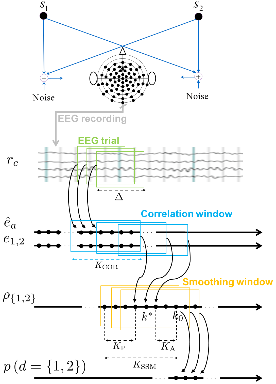
We consider an acoustic scenario comprising two competing speakers and background noise in a reverberant environment, where the ongoing EEG responses of a listener to these acoustic stimuli are recorded (See Fig. 1). The clean speech signal of speaker $1$ is denoted as $s_{1}\left[n\right]$, with $n$ the discrete time index, while the clean speech signal of speaker $2$ is denoted as $s_{2}\left[n\right]$. The envelopes of the clean speech signals of speaker $1$ and $2$ are denoted as $e_{1}\left[k\right]$ and $e_{2}\left[k\right]$, with $k$ the sub-sampled time index, respectively.

The reconstructed attended speech envelope from $C$-channel EEG recordings $r_{c}\left[k\right]$, with $c=1\ldots C$, using a trained spatio-temporal envelope estimator $F$ is given by

with

where $\Delta$ denotes the latency considered for modeling the attentional effect in the EEG responses to acoustic stimuli.

The Pearson correlation coefficients between the reconstructed attended envelope $\hat{e}_{a}\left[k\right]$ and the envelope of two speakers are given by

where $\hat{\mathbf{e}}_{a}\left[k\right]$ denotes the stacked vector of the reconstructed attended envelope corresponding to a correlation window of length $K_{\text{COR}}$, i.e.,

and $\mathbf{e}_{1}\left[k\right]$ and $\mathbf{e}_{2}\left[k\right]$ are defined similarly as in (5). Please note that in this paper we assume that the clean speech signal of speakers are available for obtaining the envelopes of speakers $e_{1}\left[k\right]$ and $e_{2}\left[k\right]$. However, since in practice only microphone signals containing a mixture of speakers and ambient noise are available, the clean speech signal of speakers needs to be appropriately estimated from microphone signals, e.g., by using the noise reduction and source separation algorithms proposed in [3, 10, 11, 2].

Suppose the attended envelope is reconstructed using a trained (linear or nonlinear) spatio-temporal estimator and the correlation coefficients of speakers are obtained. We aim at estimating the probability of attending to speaker $1$ or $2$ based on a state-space model using the past and the subsequent correlation coefficients (see Fig. 1). Let the attention state of the listener when attending to either speaker $1$ or $2$ be defined as a binary random variable, i.e.,

which follows a Bernoulli process. The probability of attending to speakers based on the state-space model is obtained as [12, 7]

with

, $c_{0}$ denoting the hyperparameter ensuring the stability of $z_{k}$, and $a_{0}$ and $b_{0}$ denoting the hyperparameters used to control the smoothing degree of the state-space model by tuning the variations of $z_{k}$ and $p\left(d_{k}=\left\{1,2\right\}\right)$. The autoregressive model in (8) implies that the (attention state) parameter $z_{k}$ at instance $k$ is predicted from $z_{k-1}$ at the instance $k-1$ with some uncertainty, which is modeled by the noise process $w\left(k\right)$. Please note that when $z_{k}$ varies from $-\infty$ to $\infty$, $p\left(d_{k}=1\right)$ monotonically varies from $0$ to $1$. To relate the correlation coefficients of speakers to the attention state, the probability of the absolute values of correlation coefficients given attending to either speaker $1$ or $2$ is modeled using a Log-Normal distribution, i.e.,

with $\boldsymbol{\alpha}_{a}$ denoting the parameter set of the attended Log-Normal distribution. The probability of the correlation coefficients given ignoring either speaker $1$ or $2$ is modeled as

with $\boldsymbol{\alpha}_{u}$ denoting the parameter set of the unattended Log-Normal distribution.

Let’s suppose we are at the instance $k=k_{0}$ (see Fig. 1) and aim to estimate the probability of attending to speakers $p\left(d_{k}=\left\{1,2\right\}\right)$ at the instance $k=k^{\ast}$ using the correlation coefficients obtained within a sliding smoothing window of length $K_{\text{SSM}}=K_{P}+K_{A}+1$, with $K_{P}$ and $K_{A}$ denoting the parameters determining the number of the correlation coefficient prior to and after the instance $k^{\ast}$, respectively. The parameters of the state-space model corresponding to the smoothing window are hence given as $\Omega=\left\{z_{k_{0}-K_{\text{SSM}}+1:k_{0}},\eta_{k_{0}-K_{\text{SSM}}+1:k_{0}},\boldsymbol{\alpha}_{a},\boldsymbol{\alpha}_{u}\right\}$. Theses parameters including $z_{k^{\ast}}$ are estimated from the correlation coefficients $\rho_{1,k_{0}-K_{\text{SSM}}+1:k_{0}}$ and $\rho_{2,k_{0}-K_{\text{SSM}}+1:k_{0}}$ obtained within the smoothing window using the Expectation Maximization (EM) estimation algorithm proposed in [12, 7]. Based on the estimated attention state parameter $z_{k^{\ast}}$, the probability of attending to speakers $p\left(d_{k^{\ast}}=\left\{1,2\right\}\right)$ are obtained. It is then decided that the listener attended to speaker 1 if $p\left(d_{k^{\ast}}=1\right)>p\left(d_{k^{\ast}}=2\right)$ or attended to speaker 2 otherwise. Please note that the estimated parameters $\Omega$ are also used for the initialization of parameters in the next smoothing window.

In the simulations (see Section 3), we will consider to use the state-space model with correlation coefficients generated either by the least-squares-based AAD method (see Section 2.3) or the neural-network-based AAD method (see Section 2.4).

The least-squares-based AAD method proposed in [4] aims at estimating the attended speech envelope from the EEG recordings using a trained linear spatio-temporal estimator. In the training step, the attended speaker is assumed to be known and an attended speech signal is used to train a linear estimator by minimizing the least-squares error between the attended speech envelope $e_{a}\left[k\right]$ and the reconstructed envelope $\hat{e}_{a}\left[k\right]$, i.e.,

with $\hat{e}_{a}\left[k\right]=F(\mathbf{r}\left[k\right])=\mathbf{g}^{T}\mathbf{r}\left[k\right]$, $\mathbf{D}$ denoting the derivative matrix [13] and $\beta$ denoting a regularization parameter. The linear estimator minimizing the regularized least-squares cost function in (13) is equal to

with the correlation matrix $\mathbf{Q}$ and the cross-correlation vector $\mathbf{q}$ given by

In the decoding step, the attended envelope $\hat{e}_{a}\left[k\right]$ is obtained using the (trained) linear estimator $\mathbf{g}$ in (14). Next, the correlation coefficients between the reconstructed attended envelope and the envelope of two speaker $\rho_{1,k}$ and $\rho_{2,k}$ are computed as in (4). Based on these correlation coefficients, it is then decided that the listener attended to speaker 1 if $\rho_{1,k}>\rho_{2,k}$ or attended to speaker 2 otherwise.

The neural-network-based AAD method aims at estimating the attended speech envelope from the EEG recordings using a trained non-linear spatio-temporal estimator. Similarly as in [8, 9], we consider a network $\mathcal{H}$ consisting of a hidden convolutional layer with hyperbolic tangent activation functions and one output layer with linear activation functions. In the training step, the network is trained to maximize the correlation between the attended speech envelope and the reconstructed envelope by minimizing the correlation cost function [8], i.e.,

A correlation cost function equal to $0$ corresponds to the maximum correlation between the attended speech envelope and the reconstructed envelope, i.e., $\rho\left(\mathbf{e}_{a}\left[k\right],\;\hat{\mathbf{e}}_{a}\left[k\right]\right)=1$, while a correlation cost function equal to $1$ corresponds to the minimum correlation. A correlation cost function larger than $1$ corresponds to a negative correlation.

In the decoding step, the attended envelope is obtained using the (trained) network $\mathcal{H}$, i.e., $\hat{e}_{a}\left[k\right]=F(\mathbf{r}\left[k\right])=\mathcal{H}(\mathbf{r}\left[k\right])$. Next, the correlation coefficients between the reconstructed attended envelope and the envelope of two speaker are computed $\rho_{1,k}$ and $\rho_{2,k}$ as in (4). Based on these correlation coefficients, it is then decided that the listener attended to speaker 1 if $\rho_{1,k}>\rho_{2,k}$ or attended to speaker 2 otherwise.

EEG responses were recorded for $18$ native German-speaking participants. Two German audio stories, uttered by two different male speakers, were simultaneously presented to the participants using insert earphones. The presented stimuli at both ears were generated by convolving the clean speech signals, i.e., the audio stories, with (non-individualized) binaural impulse responses from [14], and adding diffuse noise, generated according to [15]. The left and the right speaker were simulated at $\theta_{1}=-45^{\circ}$ and $\theta_{2}=45^{\circ}$. Eight different acoustic conditions were considered for the stimuli: one anechoic condition with no background noise, two reverberant conditions with a moderate and a large reverberation time (reverberation time $T_{60}=0.5$ s and $1$ s), two anechoic conditions with binaural input $\mathrm{SNRs}=9.0$ dB and $4.0$ dB, and three combinations of reverberation and noise. Among all participants, $8$ participants were instructed to attend to the left speaker, while $10$ participants were instructed to attend to the right speaker. Two participants were excluded from the analysis, one participant due to poor attentional performance and the other one due to a technical hardware problem. The EEG responses were recorded using $C=64$ channels at a sampling frequency of $500$ Hz, and referenced to the nose electrode. The EEG responses were re-referenced offline to a common average reference, band-pass filtered between $2$ Hz and $8$ Hz using a third-order Butterworth band-pass filter, and subsequently downsampled to $64$ Hz. The envelopes of the speech signals were obtained using a Hilbert transform, followed by low-pass filtering at $8$ Hz and downsampling to $64$ Hz.

For AAD training and testing, the EEG recordings for the different acoustic conditions were grouped together based on acoustic similarity, resulting in four experimental analysis conditions, i.e., anechoic, reverberant, anechoic-noisy, and reverberant-noisy, each of length $20$ minutes. To avoid using EEG recordings of the same experimental analysis condition for training and testing, the leave-one-condition-out approach was used, i.e., four combinations of three experimental analysis conditions without repetition were considered for training and the left condition for each combination was considered for testing. This resulted in four training conditions and four testing conditions.

For the least-squares-based AAD method, the latency parameter of the linear estimator in (3) was set to $\Delta=20$ (corresponding to $312$ ms), as found to be an appropriate choice for AAD [4, 16]. For training, the estimator in (14) and the regularization parameter $\beta$ of the estimator in (13) was determined using a k-fold cross-validation approach with $k=10$, each of length $6$ minutes. For testing, the EEG recordings were segmented into trials of length $5$ s with an overlap of $4.98$ s (corresponding to one sample shift). The correlation coefficients were computed using a correlation window of length $K_{\text{COR}}=5$ s with an overlap of $4.5$ s.

For the neural-network-based AAD method, the network $\mathcal{H}$ consisting of a convolutional hidden layer with a filter kernel size of 20 samples (corresponding to $312$ ms) was used. For training, the network was trained using a k-fold cross-validation approach with $k=10$, each of length $6$ minutes. The network was trained with the Nadam optimizer [17] using a batch size of 3840 samples (corresponding to $60$ seconds $\times$ $64$ channels), a learning rate of $0.002$, and $3000$ iterations. To avoid over-fitting, the dropout technique from [18] was used with a ratio of $0.25$, which corresponds to randomly setting $25\%$ of the hidden units to $0$. The network was implemented in Keras [19]. For testing, the correlation coefficients were obtained using the same correlation window setting as used for the least-squares-based AAD method.

For the state space model, the hyperparameters $c_{0}$ in (8) and $a_{0}$ and $b_{0}$ in (10) were set to $c_{0}=1$, $a_{0}=2.008$ and $b_{0}=0.2016$, similarly as in [7]. For testing, a sliding smoothing window of length $K_{\text{SSM}}=3$ with $K_{A}=1$, $K_{P}=1$ was used. For each testing condition, the parameter set of the attended Log-Normal distribution $\boldsymbol{\alpha}_{a}$ in (11) was initialized by fitting over correlation coefficients of the (oracle) attended speaker obtained during the first $15$ s and was then fixed. The parameter set of the unattended Log-Normal distribution $\boldsymbol{\alpha}_{u}$ in (12) was similarly initialized by fitting over correlation coefficients of the (oracle) unattended speaker. For testing, the parameters of the state-space model $\Omega$ corresponding to an smoothing window were estimated using the EM estimation algorithm with $20$ iterations.

The quality of correlation coefficients generated by either the least-squares-based AAD method or the neural-network-based AAD method was evaluated in terms of the attended correlation and the unattended correlation. The attended correlation was computed using the Pearson correlation between the reconstructed envelopes and the envelopes of the attended speaker, i.e., $\rho_{a,k}=\rho\left(\mathbf{e}_{a}\left[k\right],\;\hat{\mathbf{e}}_{a}\left[k\right]\right)$. The unattended correlation was computed between the reconstructed envelopes and the envelopes of the unattended speaker, i.e. $\rho_{u,k}=\rho\left(\mathbf{e}_{u}\left[k\right],\;\hat{\mathbf{e}}_{a}\left[k\right]\right)$,

The decoding performance was evaluated for several AAD methods, i.e., the least-squares-based AAD method (LS), the neural-network-based AAD method (NN), the state-space model using with the least-squares-based AAD method (LS-SSM) and the state-space model with the neural-network-based AAD method (NN-SSM). The decoding performance for the least-squares-based and the neural-network-based AAD method was computed as the percentage of correctly decoded $5$-second correlation windows. The decoding performance for the state-space model using either the least-squares-based or the neural-network-based AAD method was computed as the percentage of correctly decoded $5$-second smoothing windows.

References

- [1] J. O’Sullivan, Z. Chen, J. Herrero, G. M. McKhann, S. A. Sheth, A. D. Mehta, and N. Mesgarani, “Neural decoding of attentional selection in multi-speaker environments without access to clean sources,” Journal of Neural Engineering, vol. 14, no. 5, p. 56001, 2017.
- [2] S. Van Eyndhoven, T. Francart, and A. Bertrand, “EEG-informed attended speaker extraction from recorded speech mixtures with application in neuro-steered hearing prostheses,” IEEE Transactions on Biomedical Engineering, vol. 64, no. 5, pp. 1045–1056, 2017.
- [3] A. Aroudi and S. Doclo, “Cognitive-driven binaural beamforming using EEG-based auditory attention decoding,” IEEE Transactions on Audio, Speech, and Language Processing, in press.
- [4] J. A. O’Sullivan, A. J. Power, N. Mesgarani, S. Rajaram, J. J. Foxe, B. G. Shinn-Cunningham, M. Slaney, S. A. Shamma, and E. C. Lalor, “Attentional selection in a cocktail party environment can be decoded from single-trial EEG,” Cerebral Cortex, 2014.
- [5] D. D. Wong, S. A. Fuglsang, J. Hjortkjær, E. Ceolini, M. Slaney, and A. de Cheveigné, “A comparison of regularization methods in forward and backward models for auditory attention decoding,” Frontiers in Neuroscience, vol. 12, p. 531, 2018. [Online]. Available: https://www.frontiersin.org/article/10.3389/fnins.2018.00531
- [6] E. Alickovic, T. Lunner, F. Gustafsson, and L. Ljung, “A tutorial on auditory attention identification methods,” Frontiers in Neuroscience, vol. 13, p. 153, 2019.
- [7] S. Miran, S. Akram, A. Sheikhattar, J. Z. Simon, T. Zhang, and B. Babadi, “Real-time tracking of selective auditory attention from M/EEG: A Bayesian filtering approach,” Frontiers in Neuroscience, vol. 12, p. 262, 2018.
- [8] T. de Taillez, B. Kollmeier, and B. T. Meyer, “Machine learning for decoding listeners� attention from electroencephalography evoked by continuous speech,” European Journal of Neuroscience, Dec. 2018.
- [9] G. Ciccarelli, M. Nolan, J. Perricone, P. T. Calamia, S. Haro, J. O’Sullivan, N. Mesgarani, T. F. Quatieri, and C. J. Smalt, “Comparison of two-talker attention decoding from EEG with nonlinear neural networks and linear methods,” Scientific Reports, Nature, vol. 9, no. 11538, Aug. 2019.
- [10] A. Aroudi and S. Doclo, “Cognitive-driven binaural LCMV beamformer using EEG-based auditory attention decoding,” in Proc. IEEE International Conference on Acoustics, Speech and Signal Processing (ICASSP), Brighton, United Kingdom, May 2019, pp. 406–410.
- [11] C. Han, J. O’Sullivan, Y. Luo, J. Herrero, A. D. Mehta, and N. Mesgarani, “Speaker-independent auditory attention decoding without access to clean speech sources,” Science Advances, vol. 5, no. 5, 2019.
- [12] S. Akram, J. Z. Simon, and B. Babadi, “Dynamic estimation of the auditory temporal response function from MEG in competing-speaker environments,” IEEE Transactions on Biomedical Engineering, vol. 64, no. 8, pp. 1896–1905, 2017.
- [13] A. Aroudi and S. Doclo, “EEG-based auditory attention decoding using unprocessed binaural signals in reverberant and noisy conditions,” in Proc. Int. Conf. of the IEEE Engineering in Medicine and Biology Society (EMBC), Jeju, South Korea, 2017, pp. 484–488.
- [14] H. Kayser, S. D. Ewert, J. Anemüller, T. Rohdenburg, V. Hohmann, and B. Kollmeier, “Database of multichannel in-ear and behind-the-ear head-related and binaural room impulse responses,” EURASIP Journal on Advances in Signal Processing, vol. 2009, p. 6, 2009.
- [15] E. Habets, I. Cohen, and S. Gannot, “Generating nonstationary multisensor signals under a spatial coherence constraint,” Journal of the Acoustical Society of America, vol. 124, no. 5, pp. 2911–2917, Nov. 2008.
- [16] A. Aroudi, B. Mirkovic, M. De Vos, and S. Doclo, “Impact of different acoustic components on EEG-based auditory attention decoding in noisy and reverberant conditions,” IEEE Transactions on Neural Systems and Rehabilitation Engineering, vol. 27, no. 4, pp. 652–663, April 2019.
- [17] T. Dozat, “Incorporating nesterov momentum into adam,” in International Conference on Learning Representations (ICLR 2016 workshop), 2016.
- [18] N. Srivastava, G. Hinton, A. Krizhevsky, I. Sutskever, and R. Salakhutdinov, “Dropout: A simple way to prevent neural networks from overfitting,” Journal of Machine Learning Research, vol. 15, pp. 1929–1958, 2014.
- [19] F. Chollet et al., “Keras,” https://keras.io, 2015.
- [20] Y. Hochberg and A. C. Tamhane, Multiple Comparison Procedures. John Wiley and Sons, 1987.