3D Marchenko applications: Implementation and examplesSenai Cimatec, Av. Orlando Gomes 2845, Salvador, Bahia, 41650-010, Brazil

The implementation that is used in this paper makes use of a single compute kernel. By considering Equations (8) and (9), it can be seen that both of these equations make use of the same operation, namely a convolution of the reflection response or its time-reversal with either the downgoing or upgoing focusing function, followed by an application of the time window $\Theta$. It is more efficient to perform the convolution in the frequency domain, while the time window is applied in the time domain. We therefore consider these two operations separately in the kernel. Because the kernel is the same for both Equations (8) and (9), the equations can be written as a series expansion, similar to Equations (B-4) and (B-5) of Wapenaar et al., 2014b

	$\displaystyle-f_{1,k}^{-}({\bf x}_{R},{\bf x}_{A},-t)$	$\displaystyle=\sum_{i=0}^{k}N_{2i}({\bf x}_{A},{\bf x}_{R},t),$		(11)
	$\displaystyle f^{+}_{1,k+1}({\bf x}_{R},{\bf x}_{A},t)$	$\displaystyle=\sum_{i=0}^{k}N_{2i+1}({\bf x}_{A},{\bf x}_{R},t)+f_{1,d}^{+}({\bf x}_{R},{\bf x}_{A},t)=\sum_{i=-1}^{k}N_{2i+1}({\bf x}_{A},{\bf x}_{R},t),$		(12)

where

$\displaystyle N_{i}({\bf x}_{A},{\bf x}_{R},-t)$

$\displaystyle=-\Theta RN_{i-1}({\bf x}_{A},{\bf x}_{R},t),$

(13)

$\displaystyle RN_{i-1}({\bf x}_{A},{\bf x}_{R},\omega)$

$\displaystyle=\sum^{n_{S}}_{j=1}R({\bf x}_{R},{\bf x}_{S,j},\omega)N_{i-1}({\bf x}_{A},{\bf x}_{S,j},\omega)\frac{\Delta x_{1}\Delta x_{2}\Delta t}{n_{t}},$

(14)

$\displaystyle N_{-1}({\bf x}_{A},{\bf x}_{R},t)$

$\displaystyle=f_{1,d}^{+}({\bf x}_{R},{\bf x}_{A},t).$

(15)

Equation (14) is performed in the frequency domain and therefore the functions depend on the angular frequency $\omega$ instead of time. The data are transformed to the frequency domain using the Fourier transform and as a result, the convolution between the reflection response and $N_{i}$ becomes a simple multiplication. To account for the discrete Fourier transform, the data needs to be divided by the number of time samples $n_{t}$ and a scaling with the temporal sampling $\Delta t$ is required for the numerical time convolution. We have also replaced the integral over the source locations by a numerical approximation, namely a sum over the source positions, where ${\bf x}_{S,j}$ indicates the $j$-th source location of a total of $n_{S}$ source locations. Furthermore, for this approximation the data need to be scaled by the spatial sampling in the horizontal direction $x_{1}$ and $x_{2}$. $\Delta x_{1}$ and $\Delta x_{2}$ indicate the spatial sampling at ${\bf x}_{S,j}$ in horizontal direction $x_{1}$ and $x_{2}$, respectively and can be different. For the 2D implementation, $\Delta x_{2}$ can be dropped and the scaling only depends on one horizontal direction.

The basic algorithm that is described by Equations (8)-(14) is the same as was used in the 2D implementation by Thorbecke et al., 2017 and the implementation is very similar, as the only addition is the integration along the second horizontal direction. However, there are additional complications that come with the 3D extension.

First, $R({\bf x}_{R},{\bf x}_{S},\omega)$ has to be considered. The 3D reflection data must be pre-processed to comply with the assumptions made in the derivation of the Marchenko equations Wapenaar et al., 2014a. This processing has to at least include Brackenhoff et al., 2019b;

• •

  removal of free-surface multiples,

• •

  deconvolution with source wavelet,

• •

  crossline interpolation to avoid aliasing.

The removal of free-surface multiples and the deconvolution of the wavelet is beyond the scope of this paper, however, the crossline interpolation is a relevant topic as it relates to one of the most critical requirements of the reflection data, namely dense spatial sampling. Our implementation assumes that this requirement has been fulfilled, however, as a result the size of the reflection data will become very large. Loading the pre-processed reflection data from disk to memory is generally an inexpensive task in 2D, however, loading the full 3D reflection data matrix takes much longer and the storage space that is required for the data is much larger. To mitigate these problems a ZFP based compression algorithm is used (Lindstrom, 2014). The ZFP compression has been succesfully applied for the purpose of reducing the data size of seismic waveforms for waveform tomography with minimal errors (Lindstrom et al., 2016). Before the reflection data are compressed, they are transformed to the frequency domain, as the reflection data are only used in the frequency domain to circumvent the convolution, and only the data in the frequency-band of interest are compressed and stored to disk. Typically the lossless ZFP compression reduces the 3D data size by a factor of 4, which decreases the storage space of the data and the read-in time to memory. The program TWtransform (explained in appendix A.2) transforms uncompressed reflection time-data to the frequency domain, applies ZFP compression (based on tolerance) on a selected frequency range and writes the compressed data to disk. The data on disk contain a special compressed header that includes all location information present in the uncompressed Segy/SU headers that are needed in the 3D Marchenko program. The 3D Marchenko program has multiple options to read the reflection data, which can be done in the time-domain, frequency-domain, or compressed frequency-domain. In appendix A.1, the most important options and parameter settings of the 3D Marchenko program, marchenko3D, are explained in more detail.

Aside from the reflection data, the first estimation of the focusing function is also required, as dictated by Equation (15). To model this first arrival, a background velocity model is required. Using this model, the first arrival can be calculated using, for example, a finite-difference modeling code. In this paper, we make use of a 3D finite-difference modeling code fdelmodc3D that can be found in the OpenSource library by Thorbecke and Brackenhoff, 2019. While the calculation of a single first arrival is feasible using a finite-difference code, it is very computationally expensive to calculate it for a large amount of focal points in this way. Furthermore, storing all these wavefields separately would require a large amount of storage space. As an alternative to the finite-difference modeling, an Eikonal, or ray-based solver can be employed. Using this solver, the first arrival of multiple focal locations can be efficiently computed and stored on disk. We employ the Eikonal solver raytime3D from the OpenSource library to calculate these first arrivals. This code is based on the theory by Vidale, 1990 and aside from the calculation of the arrival time, it also estimates a geometric spreading factor of the wavefield, based on the concepts by Spetzler and Angelov, 2005. This amplitude estimation is important, as a uniform amplitude for all arrival times would cause significant artifacts in the result of the Marchenko method. This amplitude estimation is not exact and effects, such as transmission losses, are not taken into account, therefore there will be errors introduced in the amplitude of the estimated Green’s function. The first arrival times that are estimated, either through the finite-difference modeling code or the Eikonal solver, are also used to construct the time window $\Theta$.

When the reflection data, time window and the first arrival are available, they can be used to compute the the focusing functions through the use of Equations (8)-(14). When the iterative scheme has converged to a solution, the final estimations of the upgoing and downgoing focusing functions can be used in Equations (1) and (2) to compute the decomposed Green’s functions. The marchenko3D program has the same functionality as its 2D counterpart marchenko to run multiple focal locations simultaneously, which means that the 3D reflection data only have to be read from the disk once. This is especially useful in 3D as loading the 3D reflection data from disk takes up a significant portion of time compared to the computing time of the Marchenko method.

First, we consider the most basic application of the Marchenko method, namely, Green’s function retrieval for a point source. To generate the necessary first arrival, we model a point source at ${\bf x}_{A}=(0,0,1025)$m using an 11Hz Ricker wavelet and record the response at the surface of the medium. We separate the first arrival from the coda of the wavefield to obtain $G_{d}({\bf x}_{R},{\bf x}_{A},t)$. Instead of simply time-reversing this first arrival, we instead invert it to obtain the true $f^{+}_{1,d}({\bf x}_{R},{\bf x}_{A},t)$, which is shown in Figure 2(a). In the field, it is unlikely that we would be able to achieve this, as one would need to have the exact model available, however, here we wish to demonstrate that the method can theoretically retrieve accurate amplitudes. We use the marchenko3D code to retrieve the decomposed focusing functions and Green’s functions. We obtain the total focusing function $f_{2}({\bf x}_{A},{\bf x}_{R},t)$ and the total Green’s function $G({\bf x}_{R},{\bf x}_{A},t)$ using Equations (3) and (4), respectively and show these functions in Figure 2(b) and (c).

The convergence rate of the Marchenko method for a point source at ${\bf x}_{A}=(0,0,1025)$m is shown in Figure 3 as the solid red curve. This convergence rate is defined as the rate of the $L_{1}$ norm of the total energy in the update $N_{i}$ from Equation (13) to that of the $L_{1}$ norm of the total energy in the original update $N_{0}$. Note that a significant amount of iterations is required for convergence and that the convergence curve seems to flatten out instead of converging to zero. The low convergence rate has to do with the complexity of the model. Due to the fact that the model contains a large amount of reflectors and has a great variety of structures, the amount of iterations that are required is high. The maximum convergence is related to the aperture of the reflection response. The convergence to a relatively high energy level indicates that many limited-aperture artefacts are present in the update fields $N_{i}$. These limited-aperture effects are caused by the acquisition footprint, especially in the crossline direction. The complexity of the model causes scattering at large angles, which means that a larger aperture is required to properly capture all the scattered events. This is caused by the assumption of the Marchenko method that $\mathbb{S}_{0}$ extends infinitely in the horizontal directions, whereas in the field, it will always be limited.

To determine whether the retrieved Green’s function is accurate, we compare it to a reference Green’s function $G_{\rm ref}({\bf x}_{R},{\bf x}_{A},t)$. This Green’s function was obtained by modeling the source directly at ${\bf x}_{A}=(0,0,1025)$m and recording the response at the surface of the medium. It is shown in Figure 2(d). A visual inspection between the retrieved Green’s function and the reference Green’s function shows that the two wavefields appear to be similar, with a strong correlation between the arrival times and amplitudes of the events. The convergence to the correct solution is further supported by the decrease in energy per update, which can be interpreted from the solid red curve in Figure 3.

To make a more accurate comparison, we show a direct comparison between some of the traces of the two functions in Figure 4. The traces of the retrieved Green’s function are shown in black, while the traces of the reference Green’s function are shown in dashed red. Note that in this display, we apply a time gain of $t^{1.6}$ to boost the amplitude of the events at later times. When the traces are compared, it can be seen that the match is excellent. The traces in Figure 4(a), which have a fixed offset in the crossline $x_{2}$ direction of 500m, are nearly identical for the two functions. There is a very slight error before the first event, which is caused by the window, and at high offsets from the source position the quality of the retrieved Green’s function decreases slightly. This is because the events that have to be retrieved at this offset are not all captured by the recording aperture. This effect can be seen in Figure 4-(b), where the inline $x_{1}$ offset is fixed at 1500m. The errors are slightly larger here due to the fact that the entire panel is closer to the edge of the aperture. However, overall the match is still very strong and this demonstrates the capability of the Marchenko method to properly retrieve the Green’s function from surface reflection data.

The Green’s functions and focusing functions that are retrieved by using the Marchenko method can be employed for a variety of schemes. One of the most commonly used applications is imaging, where one aims to obtain the reflectivity of the subsurface in a region of interest. The reflectivity of the medium $\bar{R}_{\rm tar}({\bf x}_{B},{\bf x}_{A},t)$ at a target depth is related to the decomposed Green’s functions as (Amundsen, 2001; Wapenaar et al., 2014b)

$$G^{-,+}({\bf x}_{B},{\bf x}_{R},t)=\int_{\mathbb{S}_{A}}\int_{0}^{\infty}\bar{R}_{\rm tar}({\bf x}_{B},{\bf x}_{A},t-t^{\prime})G^{+,+}({\bf x}_{A},{\bf x}_{R},t^{\prime})\text{d}t^{\prime}\text{d}{\bf x}_{B},$$

(16)

where $\mathbb{S}_{A}$ is a surface inside the medium at the top of the target zone and the reciprocity relations $G^{-,+}({\bf x}_{B},{\bf x}_{R},t)=G^{-,+}({\bf x}_{R},{\bf x}_{B},t)$ and $G^{+,+}({\bf x}_{A},{\bf x}_{R},t)=G^{-,-}({\bf x}_{R},{\bf x}_{A},t)$ have been employed (Wapenaar, 2020). Through the use of a Multi-Dimensional Deconvolution (MDD) process, the reflectivity can be obtained from the decomposed Green’s functions that are obtained using the Marchenko method. By employing this process, the overburden above the target depth is removed and only interactions from the target zone below $\mathbb{S}_{A}$ are preserved. Furthermore, if there are any errors present in the amplitude of $f_{1,d}^{+}$, the same errors will be present in both $G^{-,+}$ and $G^{-,-}$, so these errors will be removed for the larger part by the MDD process. However, properly applying the MDD, especially for 3D recording setups, is very difficult and prone to errors (Staring et al., 2018). A more stable way of obtaining the reflectivity is through the use of the double-focusing method (van der Neut et al., 2018). Here, no MDD is applied, and the decomposed focusing function is used. The double-focusing method can be expressed as

$$R_{\rm tar}({\bf x}_{B},{\bf x}_{A},t)=\int_{\mathbb{S}_{0}}\int_{0}^{\infty}F^{+}({\bf x}_{R},{\bf x}_{B},t^{\prime})G^{-,+}({\bf x}_{R},{\bf x}_{A},t-t^{\prime})\text{d}t^{\prime}\text{d}{\bf x}_{R},$$

(17)

with

$$\partial_{t}F^{+}({\bf x}_{R},{\bf x}_{B},t)=-\frac{2}{\rho}\partial_{3}f_{1}^{+}({\bf x}_{R},{\bf x}_{B},t).$$

(18)

In Equation (17), $R_{\rm tar}({\bf x}_{B},{\bf x}_{A},t)=G^{-,+}({\bf x}_{B},{\bf x}_{A},t)$. Unlike the MDD approach, the double-focusing approach does not remove the overburden, but only redatums the sources and receivers from the surface of the medium to the target depth. Additionally, because there is no longer a deconvolution employed, the amplitude errors associated with $f_{1,d}^{+}$ are not removed. This means that we will not obtain the true amplitudes of the subsurface reflectors, however, we obtain the location of the reflectors, which means that we can retrieve an accurate structural image of the subsurface. The entire process is stable however, due to the fact that no deconvolution is employed. To obtain an image in a location inside the medium, without any influence of internal multiples, one can select the zero-time, zero-offset of the reflectivity in that location. This is defined as

$$r_{\rm im}({\bf x}_{B})=R_{\rm tar}({\bf x}_{B},{\bf x}_{B},t=0).$$

(19)

In this equation, the location of the virtual source and the virtual receiver coincides. For the imaging, only the first time sample is of interest. Hence, Equation (17) can be adjusted because the coda of the focusing function is meant to eliminate artifacts in the coda of the redatumed reflection response. Therefore, Equation (17) can be applied without the coda of the focusing function,

$$r_{\rm im}({\bf x}_{B})=R_{\rm tar}({\bf x}_{B},{\bf x}_{B},t=0)=\int_{\mathbb{S}_{0}}\int_{0}^{\infty}F_{d}^{+}({\bf x}_{R},{\bf x}_{B},t^{\prime})G^{-,+}({\bf x}_{R},{\bf x}_{B},-t^{\prime})\text{d}t^{\prime}\text{d}{\bf x}_{R},$$

(20)

with

$$\partial_{t}F_{d}^{+}({\bf x}_{R},{\bf x}_{B},t)=-\frac{2}{\rho}\partial_{3}f_{1,d}^{+}({\bf x}_{R},{\bf x}_{B},t).$$

(21)

In Equation (20), only the zero-time sample is retrieved, however, as stated before, the errors will be present in the coda of the redatumed reflection response and the zero time sample will be unaffected. The result can therefore also be used for the purpose of imaging without artifacts caused by internal multiples. Note that, similar to Equation (17), any errors in $f_{1,d}^{+}$ are not accounted for. The double-focusing method has been successfully employed for the purpose of imaging using 3D acquisitions in the field, for an example, see Staring and Wapenaar, 2020a.

To test the imaging potential of our marchenko3d program, we employ the double-focusing method. The required Green’s functions and focusing functions are obtained by the Marchenko method, however, we make three alterations to the approach that was used for the Green’s function retrieval. Firstly, instead of using the exact medium for estimating our first arrival, we apply a smoothing algorithm to create a background velocity model. Secondly, the first arrival is now modeled using a 3D Eikonal solver instead of using a finite-difference method. Finally, we no longer invert the first arrival, but simply take the time-reversal, as the changes to the modeling process of the first arrival will produce amplitude errors regardless. The changes in our approach are made to simulate field conditions and to keep the modeling time feasible. The Marchenko method needs to be performed for every location in the subsurface where an image is desired and therefore, the computational costs for producing an image are high.

Note that while the use of an Eikonal solver decreases the modeling time of the first arrival significantly, the use of finite-difference modeling would be a more accurate process, as an Eikonal solver does not represent the full physics of the wave equation. In media with strong velocity variations, the first arriving event may not be a purely propagating wavefield and may contain a refracted wave. The image obtained using an Eikonal solver will therefore be an approximation, however, it is computationally more feasible to apply the method like this in practice for a large amount of focal locations.

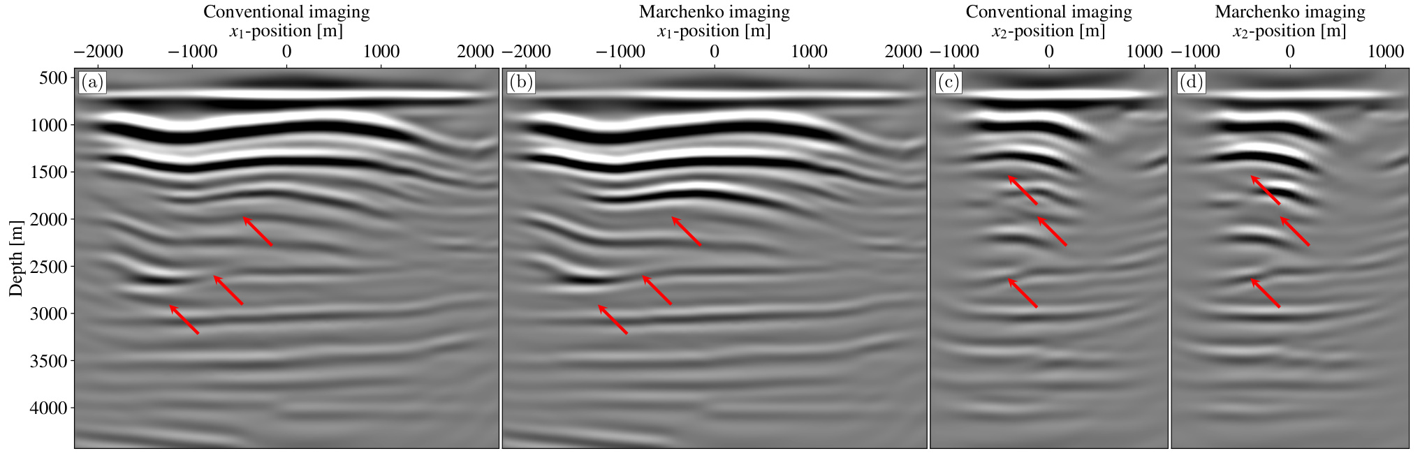
We obtain the image of two cross sections of the Overthrust model, one inline cross-section for a fixed $x_{2}$-offset of 0m and one crossline cross-section for a fixed $x_{1}$-offset of 0m. The two cross-sections intersect each other in their respective centers. The focal locations are placed along a depth range of 400 to 4400m with a sampling of 25m. The range of the focal points in the inline direction is from -2250 to 2250m, with a sampling of 25m and in the crossline direction the range is set from -1250 to 1250m with a sampling distance of 50m. Similar to the Green’s function retrieval, we perform 40 iterations for each focal point. After the focusing function and Green’s function for each focal location are obtained using the Marchenko method and Equations (1) and (2), they are used in Equation (17) to obtain the local reflectivity. The zero time sample is then extracted to obtain the reflectivity at that exact location, following Equation (19). For comparison, we also performed this approach using Equation (20) instead of (17), however, for the imaging result, there were no differences, as is expected from the theory. Figure 5(b) shows the reflectivity for each focal location for the inline direction and 5(d) shows the same for the crossline direction. Conventional images for the inline and crossline directions are shown in Figures 5(a) and 5(c), respectively. As can be seen from the figures, the subsurface is complex and hard to resolve. Due to the small frequency bandwidth, the resolution of the images is limited, however, there are still artifacts present caused by the internal multiples, as indicated by the red arrows. The Marchenko imaging attenuates these artifacts, which shows that even on complex 3D models, our marchenko3D code can produce good results. The downside is that the computational costs remain high, even if compressed reflection data are used. Imaging all the points in the inline direction for a single depth level takes around 19800 seconds or five and a half hours, running in parallel on 40 Intel E5-2560 cores with a clock speed of 2.3GHz on a node using 256GB of 2133MHz RAM. Imaging the entire 3D medium using this approach may therefore prove too demanding unless a very powerful computing machine is available. A potential solution could be the use of GPUs for the implementation of the Marchenko method, which has shown promise for 2D Marchenko applications, for example in Koehne et al., 2021

Due to the high computational costs of creating 3D images in the subsurface, it is hard to efficiently apply imaging in practice using virtual point sources. As an alternative to the standard Marchenko imaging, one can image an entire depth level at once instead of just a single point. This can be achieved through the use of virtual plane-wave sources instead of virtual point sources. The idea of combining plane-waves with the Marchenko method was first proposed by Meles et al., 2018, who applied the method with success in 2D settings. Here, we wish to implement the approach for 3D settings. The concept of the plane-wave method is that the focusing function no longer focuses to a single focal location in the subsurface, but rather to a focal depth. This gives a limited amount of information, due to the fact that only certain angles of the wavefield are considered. The plane-wave focusing functions $\tilde{f}^{\pm}_{1}({\bf x},{\bf p}_{A},t)$ are related to the focusing functions as

$$\tilde{f}^{\pm}_{1}({\bf x},{\bf p}_{A},t)=\int_{\mathbb{S}_{A}}f^{\pm}_{1}({\bf x},{\bf x}_{A},t-{\bf p}\cdot{\bf x}_{{\rm H},A}){\rm d}{\bf x}_{A},$$

(22)

where ${\bf x}_{{\rm H},A}=(x_{1,A}-x_{1,c},x_{2,A}-x_{2,c})$, ${\bf p}=(p_{1},p_{2})$ and ${\bf p}_{A}=({\bf p},x_{3,A})$. Here, $p_{1}={\rm sin}\alpha{\rm cos}\beta/c$ and $p_{2}={\rm sin}\alpha{\rm sin}\beta/c$ are the horizontal ray parameters, where $\alpha$ is the dip angle, $\beta$ is the azimuth angle and $c=c({\bf x})$ is the propagation velocity of the medium. $x_{1,c}$ and $x_{2,c}$ are the horizontal coordinates of the central location of the plane-wave source. By including these coordinates in the definition of ${\bf x}_{{\rm H},A}$, we ensure that the center of the plane-wave source always has an emission time of $t=0$. Equation (22) states that the plane-wave focusing function $\tilde{f}^{\pm}_{1}$ is the integral of the focusing functions ${f}_{1}^{\pm}$ over all possible focal points ${\bf x}_{A}$ at $\mathbb{S}_{A}$ for a certain dip and azimuth given by the ray parameters. As such, $\tilde{f}^{\pm}_{1}({\bf x},{\bf p}_{A},t)$ does not focus to a single location, but instead focuses as a dipping wave, dictated by ${\bf p}$, to a single depth level $x_{3,A}$. In case the ray parameters are zero, this wave is horizontal instead of dipping.

We also define the plane-wave Green’s functions $\tilde{G}^{-,\pm}({\bf x}_{R},{\bf p}_{A},t)$ which are related to the Green’s functions

$$\tilde{G}^{-,\pm}({\bf x}_{R},{\bf p}_{A},t)=\int_{\mathbb{S}_{A}}G^{-,\pm}({\bf x}_{R},{\bf x}_{A},t-{\bf p}\cdot{\bf x}_{{\rm H},A}){\rm d}{\bf x}_{A}.$$

(23)

The plane-wave Green’s functions behave similarly to the regular Green’s functions, however, instead of being the impulse response of a point source, the plane-wave Green’s functions are the response of a medium to a plane-wave source at $x_{3,A}$, which generates a dipping wave as dictated by the ray parameters.

The plane-wave versions of the focusing functions and the Green’s functions can be combined with the Equations (1) and (2) simply by applying the integration over all possible focal points for a set of ray parameters

	$\displaystyle\tilde{G}^{-,+}({\bf x}_{R},{\bf p}_{A}^{\prime},t)+\tilde{f}_{1}^{-}({\bf x}_{R},{\bf p}_{A}^{\prime},t)$	$\displaystyle=\int_{\mathbb{S}_{0}}\int_{0}^{\infty}R({\bf x}_{R},{\bf x}_{S},t^{\prime})\tilde{f}_{1}^{+}({\bf x}_{S},{\bf p}_{A}^{\prime},t-t^{\prime}){\rm d}t^{\prime}{\rm d}{\bf x}_{S},$		(24)
	$\displaystyle\tilde{G}^{-,-}({\bf x}_{R},{\bf p}_{A},-t)+\tilde{f}_{1}^{+}({\bf x}_{R},{\bf p}_{A}^{\prime},t)$	$\displaystyle=\int_{\mathbb{S}_{0}}\int_{-\infty}^{0}R({\bf x},{\bf x}_{S},-t^{\prime})\tilde{f}_{1}^{-}({\bf x}_{S},{\bf p}_{A}^{\prime},t-t^{\prime}){\rm d}t^{\prime}{\rm d}{\bf x}_{S}.$		(25)

In these equations, we define ${\bf p}_{A}^{\prime}=(-{\bf p},x_{3,A})$, which all plane-wave wavefields contain with the exception of $\tilde{G}^{-,-}({\bf x}_{R},{\bf p}_{A},-t)$. This is due to the fact that this particular wavefield is time-reversed in Equation (2). The change to plane-waves has not affected the reflection response, only the focusing functions and Green’s functions, which means that no changes to the reflection response have to be made. Similarly to the original equations, the Green’s functions in the system of Equations (24) and (25) can be suppressed through the use of a windowing function. The change to plane-waves does affect the causality relations however, especially because $\tilde{G}^{-,-}({\bf x}_{R},{\bf p}_{A},t)$ and $\tilde{G}^{-,+}({\bf x}_{R},{\bf p}_{A}^{\prime},t)$ are dipping at different angles. Hence, the time window needs to be adjusted so the dipping plane-waves are properly handled (Meles et al., 2020). These windows are defined as

$$\begin{split}\tilde{\Theta}=\tilde{\Theta}({\bf x}_{R},{\bf p}_{A},t)&=\theta(t-t_{a})-\theta(t-t_{b}),\\ t_{a}&=-\tilde{t}_{d}({\bf x}_{R},{\bf p}_{A})+\epsilon,\\ t_{b}&=\tilde{t}_{d}({\bf x}_{R},{\bf p}_{A}^{\prime})-\epsilon,\end{split}$$

(26)

where $\tilde{t}_{d}({\bf x}_{R},{\bf p}_{A}^{\prime})$ is the first possible arriving event of $\tilde{G}^{-,+}({\bf x}_{R},{\bf p}_{A}^{\prime},t)$ and $-\tilde{t}_{d}({\bf x}_{R},{\bf p}_{A})$ is the last arriving event of $\tilde{G}^{-,-}({\bf x}_{R},{\bf p}_{A},-t)$. As a result, the windowing function is no longer symmetrical in time, instead, the window has parallel planes. For a further derivation of this window, see Wapenaar et al., 2021. Applying this window to Equations (24) and (25) results in the plane-wave coupled Marchenko equations

	$\displaystyle\tilde{f}_{1}^{-}({\bf x}_{R},{\bf p}_{A}^{\prime},t)$	$\displaystyle=\tilde{\Theta}\int_{\mathbb{S}_{0}}\int_{0}^{\infty}R({\bf x}_{R},{\bf x}_{S},t^{\prime})\tilde{f}_{1}^{+}({\bf x}_{S},{\bf p}_{A}^{\prime},t-t^{\prime}){\rm d}t^{\prime}{\rm d}{\bf x}_{S},$		(27)
	$\displaystyle\tilde{f}_{1}^{+}({\bf x}_{R},{\bf p}_{A}^{\prime},t)-\tilde{f}_{1,d}^{+}({\bf x}_{R},{\bf p}_{A}^{\prime},t)$	$\displaystyle=\tilde{\Theta}\int_{\mathbb{S}_{0}}\int_{-\infty}^{0}R({\bf x}_{R},{\bf x}_{S},-t^{\prime})\tilde{f}_{1}^{-}({\bf x}_{S},{\bf p}_{A}^{\prime},t-t^{\prime}){\rm d}t^{\prime}{\rm d}{\bf x}_{S}.$		(28)

Note that Equations (27) and (28) have a very similar structure to Equations (6) and (7). They can therefore be solved with the same Marchenko method as was used for the point source focusing functions. The only things that have to be adjusted are the input and the windowing function. The first estimation of the focusing function can once again be estimated by using the direct arrival

$\displaystyle\tilde{f}_{1,0}^{+}({\bf x}_{R},{\bf p}_{A}^{\prime},t)=\tilde{f}^{+}_{1,d}({\bf x}_{R},{\bf p}_{A}^{\prime},t).$

(29)

However, because we cannot compute this first arrival directly, we have to model the direct arrival of the Green’s function and time-reverse it. The plane-wave is modeled by placing point sources along a horizontal plane in the medium of interest and emitting with a time delay, so that the emission time of a location along the horizontal plane is $\delta(t-{\bf p}\cdot{\bf x}_{{\rm H},A})$. By taking the direct arrival of the Green’s function, we obtain $\tilde{G}^{+}_{d}({\bf x}_{R},{\bf p}_{A},t)$, which we can then relate to the direct arrival of the focusing function as

$\displaystyle\tilde{f}^{+}_{1,d}({\bf x}_{R},{\bf p}_{A}^{\prime},t)$

$\displaystyle=\tilde{G}_{d}({\bf x}_{R},{\bf p}_{A},-t).$

(30)

Notice that according to Equation (30), the original ray parameters that were used to model the plane-wave source and obtain $\tilde{G}_{d}({\bf x}_{R},{\bf p}_{A},t)$ are the opposite of the ray parameters that are included in the first estimation of the focusing function $\tilde{f}^{+}_{1,d}({\bf x}_{R},{\bf p}_{A}^{\prime},t)$. Hence, when we use Equation (25) to obtain $\tilde{G}^{-,-}({\bf x}_{R},{\bf p}_{A},t)$, it is dipping according to the original ray parameters and when we use Equation (24) to obtain $\tilde{G}^{-,+}({\bf x}_{R},{\bf p}_{A}^{\prime},t)$ it is dipping according to the opposite of the original ray parameters.

We retrieve the Green’s function in the subsurface at a depth level of $x_{3}=1025$m. We use a plane-wave that is dipping in both the inline and the crossline direction as determined by ray parameters ${\bf p}=(80,40)\mu$s m^-1. Because the velocity of the medium varies at this depth, we cannot convert this to a single angle, however, the majority of this depth level corresponds to a velocity of 4500 m s^-1. Using this velocity we calculate a representative dip and azimuth angle, namely $\alpha=23.6^{\circ}$ and $\beta=26.6^{\circ}$. In order to obtain the full Green’s function, we run the Marchenko method twice, once using ${\bf p}$ to obtain $\tilde{G}^{-,-}({\bf x}_{R},{\bf p}_{A},t)$ and once using $-{\bf p}$ to obtain $\tilde{G}^{-,+}({\bf x}_{R},{\bf p}_{A},t)$ , and use these results in Equation (4). The initial estimation of the focusing function $\tilde{f}^{+}_{1,d}({\bf x}_{R},{\bf p}_{A}^{\prime},t)$, which we obtained in the exact model for accurate amplitudes, is shown in Figure 6(a), while the full focusing function $\tilde{f}_{2}({\bf p}_{A}^{\prime},{\bf x}_{R},t)$ is shown in (b). To construct this focusing function, we apply the plane-wave definition to Equation (3),

$$\tilde{f}_{2}({\bf p}_{A}^{\prime},{\bf x}_{R},t)=\tilde{f}_{1}^{+}({\bf x}_{R},{\bf p}_{A}^{\prime},t)-\tilde{f}_{1}^{-}({\bf x}_{R},{\bf p}_{A},-t).$$

(31)

The convergence of the Marchenko method using ${\bf p}$ is shown as the dashed blue curve in Figure 3. If $-{\bf p}$ is used, the graph is visually identical. Note that the method converges much faster if a plane-wave source is used instead of a point source, this is caused by the fact that only certain angles are covered by the dipping plane-wave, hence the amount of propagation directions that needs to be resolved is much lower. The full Green’s function $\tilde{G}({\bf x}_{R},{\bf p}_{A},t)$, which is obtained through the use of the two runs of the Marchenko method is shown in Figure 6(c).

We compare the retrieved Green’s function to a reference Green’s function $\tilde{G}_{\rm ref}({\bf x}_{R},{\bf p}_{A},t)$, that was directly modeled in the medium and is shown in Figure 6(d). Visually, the two Green’s functions appear to be very similar. There are some slight differences caused by curving events originating from the edges of the aperture. These are caused by the modeling of the plane-wave source as opposed to a point source. The amplitude along the wavefront is nearly constant for a plane-wave source, while for a point source it decreases near the edges. Therefore, the edge effects are more pronounced for the plane-wave sources. When the first arrival is isolated from the coda, these effects are largely removed, because they are present in the coda, hence the difference in the results.

To further investigate the accuracy of the retrieved Green’s function, we construct a similar figure as Figure 4, where we display traces of the two Green’s function next to each other. The result is shown in Figure 7. The accuracy has decreased in comparison with the standard point-source Green’s function retrieval, which is also a result from the plane-wave setup. The errors caused by placing the source near the edges contribute more to the final result than when point sources are used, hence the decrease in quality. Overall, the match is still very strong, for both the amplitude and the phase of the events.

We perform plane-wave imaging through the double-focusing method, similar to Equation (17). We apply the integral over all possible focal points, following Equations (22) and (23),

$$\tilde{R}_{\rm tar}({\bf x}_{B},{\bf p}_{A},t)=\int_{\mathbb{S}_{0}}\int_{0}^{\infty}F^{+}({\bf x}_{R},{\bf x}_{B},t^{\prime})\tilde{G}^{-,+}({\bf x}_{R},{\bf p}_{A},t-t^{\prime})\text{d}t^{\prime}\text{d}{\bf x}_{R}.$$

(32)

In Equation (32), $\tilde{G}^{-,+}$ and $\tilde{R}_{\rm tar}$ are both plane-wave responses, while $F^{+}$ still is the focusing function related to a focal point instead of a focal depth. We can use the redatumed receiver response to formulate an image condition for each location in the surface

$$\tilde{r}_{\rm im}({\bf x}_{B},{\bf p}_{A})=\tilde{R}_{\rm tar}({\bf x}_{B},{\bf p}_{A},t={\bf p}\cdot{\bf x}_{{\rm H},B}).$$

(33)

Here, $\tilde{r}_{\rm im}({\bf x}_{B},{\bf p}_{A})$ is the reflectivity in the subsurface at location ${\bf x}_{B}$ given a certain angle dictated by ${\bf p}_{A}$. The time sample that is selected from the redatumed receiver response is changed, depending on the angle of the incoming wave, which is required due to the time-delay associated with the angle of the wavefront. By choosing different values for ${\bf p}_{A}$, a reflection image can be obtained for various angles.

Note that in order to obtain the correct angle-dependent reflectivity, both $F^{+}({\bf x}_{R},{\bf x}_{B},t)$ and $\tilde{G}^{-,+}({\bf x}_{R},{\bf p}_{A},t)$ need to have accurate amplitudes. As we mentioned, this is hard to achieve using the Marchenko method in practice. As a result, we will not retrieve the true angle-dependent reflectivity of the subsurface, however, we can obtain a structural image of the subsurface related to specific ray parameters. In order to obtain the true angle-dependent reflectivity, Equation (32) can be rewritten as a deconvolutional process, similar to Equation (16), but this is beyond the scope of this paper, as we are interested in efficiently obtaining a structural image of the subsurface.

The procedure using Equation (32) has a notable disadvantage in that not only the plane-wave response needs to be obtained, but also the focusing function for each focal point in the subsurface, which means that the computational effort compared to using Equation (17) in fact increases. However, if we instead use an approach similar to Equation (20), we can avoid the computation of the full focusing function. We rewrite Equation (32) combined with (33) as

$$\tilde{r}_{\rm im}({\bf x}_{B},{\bf p}_{A})=\tilde{R}_{\rm tar}({\bf x}_{B},{\bf p}_{A},t={\bf p}\cdot{\bf x}_{{\rm H},B})=\int_{\mathbb{S}_{0}}\int_{0}^{\infty}F_{d}^{+}({\bf x}_{R},{\bf x}_{B},t^{\prime})\tilde{G}^{-,+}({\bf x}_{R},{\bf p}_{A},{\bf p}\cdot{\bf x}_{{\rm H},B}-t^{\prime})\text{d}t^{\prime}\text{d}{\bf x}_{R}.$$

(34)

We only model the first arrival for each point we want to image and do not need to apply the Marchenko method to obtain the full focusing function, saving considerable computational costs.

To demonstrate the results of the method, we apply Equation (33) to the Overthrust model. We retrieve a horizontal plane-wave, i.e. ${\bf p}=(0,0)$, and image the same section as we did in Figure 5(b). The first arrival for the plane-wave $\tilde{f}^{+}_{1,d}$ is obtained through the use of finite-difference modeling, while the first arrival $f^{+}_{1,d}$ that is used in Equation (21) and subsequently in Equation (34) is obtained using the Eikonal solver. The result is shown in Figure 8(e). For comparison, for the standard Marchenko image we perform the Marchenko method for 161 depths and 181 lateral positions, for a total of 29141 different points, while for the plane-wave imaging, we perform the Marchenko method only for the 161 depths. The computation times for all these depths using plane-wave sources is around five and a half hours, which is similar to the computational time of all focal points in the inline direction for a single depth when the standard Marchenko imaging is employed. Because the first arrivals that are used for the imaging step are all obtained using an Eikonal solver, the computational costs of retrieving these events are negligible compared to the computational costs of the Marchenko method. The image that is obtained using the horizontal plane-wave contains many similar reflectors as were seen in the standard Marchenko image in Figure 5(b). However, because we are only considering reflectivity that is related to certain ray parameters, the reflectors are not as well resolved as the standard Marchenko image.

We consider additional angles of reflectivity in order to resolve the events in the plane-wave image more clearly (Meles et al., 2018). These images are shown in Figure 8, for varying ray parameters. The ray parameter in the inline direction takes values of -80, 0 and 80$\mu$s m^-1 and the ray parameter in the crossline direction takes values of -40, 0 and 40$\mu$s m^-1. The central column shows the result when the inline ray parameter is zero and we can see that these panels contain the most energy. This indicates that a large amount of the reflectors have a small dipping angle in the inline direction. The deepest part of the image also contains less energy when the crossline ray parameter is negative rather than positive, which indicates that the reflectors at this depth are dipping positively in the crossline direction. The images constructed with a negative ray parameter in the inline direction contain considerably less energy than when the ray parameter is positive. The energy is mostly constrained to the shallow part of the image and the edges. Especially near the edges it is hard to determine whether this is caused by the edge of the aperture or by genuine reflector direction. The images that have a dip in the inline direction contain more energy and have reflectors at various depths and at distances away from the edge.

Figure 8 gives insight into the reflector dip of the subsurface. We combine these results together to create a single image, which is shown in Figure 9(a). For comparison, we plot the result of the standard Marchenko image in (b). Most of the major reflectors are present at the same locations and with similar reflector strength in both imaging results. The result of the standard Marchenko imaging is better resolved, because this approach takes into account all angles of reflections within the range that is measured by the aperture. While the result of the plane-wave images is of a lesser quality, the computational costs are significantly lower, even if several images associated with different ray parameters have to be retrieved. We repeat the retrieval for both the standard Marchenko approach and plane-wave Marchenko approach to retrieve the image in the crossline direction. The result for the plane-wave Marchenko image is shown in Figure 9(c) and for the standard Marchenko image in (d). From these images we can draw similar conclusions as we did from the images in the inline direction. The same events are resolved however, the resolution of the standard Marchenko image is higher than that of the plane-wave image. It should also be noted that the plane-wave image does not contain any of the artifacts that are present when conventional imaging is used, as the plane-wave Marchenko method still attenuates all the internal multiple artifacts.

References

- Aminzadeh et al., (1997) Aminzadeh, F., Brac, J., and Kunz, T. (1997). SEG/EAGE 3-D Salt and Overthrust models. SEG/EAGE 3-D modeling series, no. 1: Distribution CD of Salt and Overthrust models. SEG book series.
- Amundsen, (2001) Amundsen, L. (2001). Elimination of free-surface related multiples without need of the source wavelet. Geophysics, 66(1):327–341.
- Ayachit, (2015) Ayachit, U. (2015). The Paraview Guide: A Parallel Visualization Application. Kitware, Inc., Clifton Park, NY.
- Behura et al., (2014) Behura, J., Wapenaar, K., and Snieder, R. (2014). Autofocus imaging: Image reconstruction based on inverse scattering theory. Geophysics, 79(3):A19–A26.
- Brackenhoff, (2016) Brackenhoff, J. (2016). Rescaling of incorrect source strength using Marchenko redatuming. M.Sc. thesis, Delft University of Technology, Delft, Zuid-Holland, the Netherlands.
- (6) Brackenhoff, J., Thorbecke, J., and Wapenaar, K. (2019a). Monitoring induced distributed double-couple sources using Marchenko-based virtual receivers. Solid Earth, 10(4):1301–1319.
- (7) Brackenhoff, J., Thorbecke, J., and Wapenaar, K. (2019b). Virtual sources and receivers in the real Earth: Considerations for practical applications. Journal of Geophysical Research: Solid Earth, 124(11):11802–11821.
- Broggini and Snieder, (2012) Broggini, F. and Snieder, R. (2012). Connection of scattering principles: A visual and mathematical tour. European Journal of Physics, 33(3):593.
- (9) Broggini, F., Snieder, R., and Wapenaar, K. (2014a). Data-driven wavefield focusing and imaging with multidimensional deconvolution: Numerical examples for reflection data with internal multiples. Geophysics, 79(3):WA107–WA115.
- (10) Broggini, F., Wapenaar, K., van der Neut, J., and Snieder, R. (2014b). Data-driven Green’s function retrieval and application to imaging with multidimensional deconvolution. Journal of Geophysical Research: Solid Earth, 119(1):425–441.
- Cohen and Stockwell, (2001) Cohen, J. and Stockwell, J. J. (2001). CWP/SU: Seismic Unix Release No. 43R4: an open source software package for seismic research and processing. Center for Wave Phenomena, Colorado School of Mines.
- da Costa Filho et al., (2014) da Costa Filho, C. A., Ravasi, M., Curtis, A., and Meles, G. A. (2014). Elastodynamic Green’s function retrieval through single-sided Marchenko inverse scattering. Phys. Rev. E, 90:063201.
- da Costa Filho et al., (2018) da Costa Filho, C. A., Tant, K., Curtis, A., Mulholland, A., and Moran, C. M. (2018). Using laboratory experiments to develop and test new marchenko and imaging methods. In 89th annual meeting SEG, 2018, pages 4352–4356. Society of Exploration Geophysicists.
- Haindl et al., (2021) Haindl, C., Ravasi, M., and Broggini, F. (2021). Handling gaps in acquisition geometries — Improving Marchenko-based imaging using sparsity-promoting inversion and joint inversion of time-lapse data. Geophysics, 86(2):S143–S154.
- Koehne et al., (2021) Koehne, V., Santos, M., Santos, R., Barrera, D., Brackenhoff, J., and Thorbecke, J. (2021). A multi-GPU benchmark for 2D Marchenko Imaging. arXiv, 2106.04649:1–13.
- Lindstrom, (2014) Lindstrom, P. (2014). Fixed-rate compressed floating-point arrays. IEEE Transactions on Visualization and Computer Graphics, 20(12):2674–2683.
- Lindstrom et al., (2016) Lindstrom, P., Chen, P., and Lee, E.-J. (2016). Reducing disk storage of full-3D seismic waveform tomography (F3DT) through lossy online compression. Computers and Geosciences, 93:45–54.
- Lomas and Curtis, (2020) Lomas, A. and Curtis, A. (2020). Marchenko methods in a 3-D world. Geophysical Journal International, 220(1):296–307.
- Marchenko, (1955) Marchenko, V. A. (1955). On reconstruction of the potential energy from phases of the scattered waves. Dokl. Akad. Nauk SSSR, 104(5):695–698.
- Matias et al., (2018) Matias, M. M. A., da C. Pestana, R., and van der Neut, J. (2018). Marchenko imaging by unidimensional deconvolution. Geophysical Prospecting, 66(9):1653–1666.
- Meles et al., (2015) Meles, G. A., Löer, K., Ravasi, M., Curtis, A., and da Costa Filho, C. A. (2015). Internal multiple prediction and removal using Marchenko autofocusing and seismic interferometry. Geophysics, 80(1):A7–A11.
- Meles et al., (2018) Meles, G. A., Wapenaar, K., and Thorbecke, J. (2018). Virtual plane-wave imaging via Marchenko redatuming. Geophysical Journal International, 214(1):508–519.
- Meles et al., (2020) Meles, G. A., Zhang, L., Thorbecke, J., Wapenaar, K., and Slob, E. (2020). Data-driven retrieval of primary plane-wave responses. Geophysical Prospecting, 68(6):1834–1846.
- Pereira et al., (2019) Pereira, R., Ramzy, M., Griscenco, P., Huard, B., Huang, H., Cypriano, L., and Khalil, A. (2019). Internal multiple attenuation for OBN data with overburden/target separation. In 90th annual meeting SEG, 2019, pages 4520–4524. Society of Exploration Geophysicists.
- Ravasi, (2017) Ravasi, M. (2017). Rayleigh-Marchenko redatuming for target-oriented, true-amplitude imaging. Geophysics, 82(6):S439–S452.
- Ravasi and Vasconcelos, (2021) Ravasi, M. and Vasconcelos, I. (2021). An open-source framework for the implementation of large-scale integral operators with flexible, modern HPC solutions - Enabling 3D Marchenko imaging by least squares inversion. Geophysics, 0:1–74.
- Ravasi et al., (2016) Ravasi, M., Vasconcelos, I., Kritski, A., Curtis, A., da Costa Filho, C. A., and Meles, G. A. (2016). Target-oriented Marchenko imaging of a North Sea field. Geophysical Journal International, 205(1):99–104.
- Reinicke, (2020) Reinicke, C. (2020). Elastodynamic Marchenko inverse scattering. Ph.D. thesis, Delft University of Technology, Delft, Zuid-Holland, the Netherlands.
- Singh et al., (2015) Singh, S., Snieder, R., Behura, J., van der Neut, J., Wapenaar, K., and Slob, E. (2015). Marchenko imaging: Imaging with primaries, internal multiples, and free-surface multiples. Geophysics, 80(5):S165–S174.
- Slob and Wapenaar, (2017) Slob, E. and Wapenaar, K. (2017). Theory for Marchenko imaging of marine seismic data with free surface multiple elimination. In 79th EAGE Conference and Exhibition, 2017. European Association of Geoscientists & Engineers.
- Slob et al., (2014) Slob, E., Wapenaar, K., Broggini, F., and Snieder, R. (2014). Seismic reflector imaging using internal multiples with Marchenko-type equations. Geophysics, 79(2):S63–S76.
- Spetzler and Angelov, (2005) Spetzler, J. and Angelov, P. (2005). Ray perturbation theory for traveltime and amplitude attributes in 3D heterogeneous media with weak anisotropy. In 75th annual meeting SEG, 2005, pages 2366–2369. Society of Exploration Geophysicists.
- Staring et al., (2018) Staring, M., Pereira, R., Douma, H., van der Neut, J., and Wapenaar, K. (2018). Source-receiver Marchenko redatuming on field data using an adaptive double-focusing method. Geophysics, 83(6):1–48.
- Staring and Wapenaar, (2019) Staring, M. and Wapenaar, K. (2019). Interbed demultiple using Marchenko redatuming on 3D field data of the Santos Basin. In 16th International Congress of the Brazilian Geophysical Society, 2019. Brazilian Geophysical Society, SBGf.
- (35) Staring, M. and Wapenaar, K. (2020a). 3D Marchenko internal multiple attenuation on narrow azimuth streamer data of the Santos Basin, Brazil. Geophysical Prospecting, 68(6):1864–1877.
- (36) Staring, M. and Wapenaar, K. (2020b). Three-dimensional Marchenko internal multiple attenuation on narrow azimuth streamer data of the Santos basin, Brazil. Geophysical Prospecting, 68(6):1864–1877.
- Thorbecke and Brackenhoff, (2019) Thorbecke, J. and Brackenhoff, J. (2019). OpenSource: Code for geophysical 3D/2D Finite Difference modelling, Marchenko algorithms, 2D/3D x-w migration and utilities. https://doi.org/10.5281/zenodo.3374728.
- Thorbecke et al., (2017) Thorbecke, J., Slob, E., Brackenhoff, J., van der Neut, J., and Wapenaar, K. (2017). Implementation of the Marchenko method. Geophysics, 82(6):WB29–WB45.
- van der Neut et al., (2018) van der Neut, J., Brackenhoff, J., Staring, M., Zhang, L., de Ridder, S., Slob, E., and Wapenaar, K. (2018). Single- and double-sided Marchenko imaging conditions in acoustic media. IEEE Transactions on Computational Imaging, 4(1):160–171.
- (40) van der Neut, J., Thorbecke, J., Wapenaar, K., and Slob, E. (2015a). Inversion of the multidimensional Marchenko equation. In 77th EAGE Conference and Exhibition, 2015. European Association of Geoscientists & Engineers.
- (41) van der Neut, J., Vasconcelos, I., and Wapenaar, K. (2015b). On Green’s function retrieval by iterative substitution of the coupled Marchenko equations. Geophysical Journal International, 203(2):792–813.
- van der Neut and Wapenaar, (2016) van der Neut, J. and Wapenaar, K. (2016). Adaptive overburden elimination with the multidimensional Marchenko equation. Geophysics, 81(5):T265–T284.
- van Groenestijn and Verschuur, (2009) van Groenestijn, G. and Verschuur, D. (2009). Estimating primaries by sparse inversion and application to near-offset data reconstruction. Geophysics, 74(3):A23–A28.
- van IJsseldijk and Wapenaar, (2020) van IJsseldijk, J. and Wapenaar, K. (2020). Adaptation of the iterative Marchenko scheme for imperfectly sampled data. Geophysical Journal International, 224(1):326–336.
- Verschuur et al., (1992) Verschuur, D. J., Berkhout, A., and Wapenaar, C. (1992). Adaptive surface-related multiple elimination. Geophysics, 57(9):1166–1177.
- Vidale, (1990) Vidale, J. E. (1990). Finite difference calculation of traveltimes in three dimensions. Geophysics, 55(5):521–526.
- Wapenaar, (2014) Wapenaar, K. (2014). Single-sided Marchenko focusing of compressional and shear waves. Phys. Rev. E, 90:063202.
- Wapenaar, (2020) Wapenaar, K. (2020). Reciprocity and representation theorems for flux-and field-normalised decomposed wave fields. Advances in Mathematical Physics, 2020:9540135–9540150.
- Wapenaar et al., (2021) Wapenaar, K., Brackenhoff, J., Dukalski, M., Meles, G., Reinicke, C., Slob, E., Staring, M., Thorbecke, J., van der Neut, J., and Zhang, L. (2021). Marchenko redatuming, imaging and multiple elimination, and their mutual relations. Geophysics, 0:1–103.
- Wapenaar et al., (2013) Wapenaar, K., Broggini, F., Slob, E., and Snieder, R. (2013). Three-dimensional single-sided Marchenko inverse scattering, data-driven focusing, Green’s function retrieval, and their mutual relations. Physical Review Letters, 110:084301.
- (51) Wapenaar, K., Thorbecke, J., van der Neut, J., Broggini, F., Slob, E., and Snieder, R. (2014a). Green’s function retrieval from reflection data, in absence of a receiver at the virtual source position. The Journal of the Acoustical Society of America, 135(5):2847–2861.
- (52) Wapenaar, K., Thorbecke, J., van der Neut, J., Broggini, F., Slob, E., and Snieder, R. (2014b). Marchenko imaging. Geophysics, 79(3):WA39–WA57.
- Zhang and Staring, (2018) Zhang, L. and Staring, M. (2018). Marchenko scheme based internal multiple reflection elimination in acoustic wavefield. Journal of Applied Geophysics, 159:429 – 433.
- Zhou et al., (2019) Zhou, J., Zhang, W., Lei, T., Wang, D., and Li, J. (2019). Reconstructing the primaries of PP and PS waves by elastic Marchenko method. In 90th annual meeting SEG, 2019, pages 4700–4704. Society of Exploration Geophysicists.
Appendix A Input for marchenko3D and auxiliary programs
A.1 marchenko3D
The marchenko3D program has the following parameters and options:
MARCHENKO3D - Iterative Green’s function and focusing functions retrieval in 3D
marchenko3D file_tinv= file_shot= [optional parameters]
Required parameters:
First arrival input options:
file_tinv= ............... direct arrival from focal point: G_d
file_ray= ................ direct arrival from raytimes
Shot data input options:
file_shot= ............... Reflection response (time data): R(t)
file_shotw= .............. Reflection response (frequency data): R(w)
file_shotzfp= ............ Reflection response (frequency compressed data): zfp[R(w)]
Optional parameters:
INTEGRATION
ampest=0 ................. Estimate a scalar amplitude correction with depth (=1)
tap=0 .................... lateral taper focusing(1), shot(2) or both(3)
ntap=0 ................... number of taper points at boundaries
fmin=0 ................... minimum frequency in the Fourier transform
fmax=70 .................. maximum frequency in the Fourier transform
MARCHENKO ITERATIONS
niter=10 ................. number of iterations
MUTE-WINDOW
file_amp= ................ amplitudes for the raytime estimation
file_wav= ................ Wavelet applied to the raytime data
above=0 .................. mute above(1), around(0) or below(-1) the travel times of the first arrival
shift=12 ................. number of points above(positive) / below(negative) travel time for mute
hw=8 ..................... window in time samples to look for maximum in next trace
smooth=5 ................. number of points to smooth mute with cosine window
plane_wave=0 ............. enable plane-wave illumination function
src_anglex=0 ............. angle of the plane wave in the x-direction
src_angley=0 ............. angle of the plane wave in the y-direction
src_velox=0 .............. velocity of the plane wave in the x-direction
src_veloy=0 .............. velocity of the plane wave in the y-direction
REFLECTION RESPONSE CORRECTION
scale=2 .................. scale factor of R for summation of Ni with G_d (only for time shot data)
pad=0 .................... amount of samples to pad the reflection series
HOMOGENEOUS GREEN’S FUNCTION RETRIEVAL OPTIONS
file_homg= ............... output file with homogeneous Green’s function
The homogeneous Green’s function is computed if a filename is given
file_inp= ................ Input source function for the retrieval
scheme=0 ................. Scheme for the retrieval
.......................... scheme=0 Marchenko homogeneous Green’s function retrieval with G source
.......................... scheme=1 Marchenko homogeneous Green’s function retrieval with f2 source
.......................... scheme=2 Marchenko Green’s function retrieval with source depending on virtual
receiver location
.......................... scheme=3 Marchenko Green’s function retrieval with G source
.......................... scheme=4 Marchenko Green’s function retrieval with f2 source
.......................... scheme=5 Classical homogeneous Green’s function retrieval
.......................... scheme=6 Marchenko homogeneous Green’s function retrieval with multiple G sources
.......................... scheme=7 Marchenko Green’s function retrieval with multiple G sources
.......................... scheme=8 f1+ redatuming
.......................... scheme=9 f1- redatuming
.......................... scheme=10 2i IM(f1) redatuming
cp=1000.0 ................ Velocity of upper layer for certain operations
rho=1000.0 ............... Density of upper layer for certain operations
IMAGING
file_imag= ............... output file with image
The image is computed if a filename is given
OUTPUT DEFINITION
file_green= .............. output file with full Green function(s)
file_gplus= .............. output file with G+
file_gmin= ............... output file with G-
file_f1plus= ............. output file with f1+
file_f1min= .............. output file with f1-
file_f2= ................. output file with f2
file_ampscl= ............. output file with estimated amplitudes
file_iter= ............... output file with -Ni(-t) for each iteration
compact=0 ................ Write out homg and imag in compact format
.......................... WARNING! This write-out cannot be displayed with SU
zfp=0 .................... Write out the standard output in compressed zfp format
tolerance=1e-7 ........... accuracy of the zfp compression,
verbose=0 ................ silent option; >0 displays info
The input of the 3D Marchenko method is similar to the 2D implementation, requiring reflection data and the first arrival time from the focal point. However, due to the large size of 3D data, loading the reflection data from disk using the file_shot option can become time-consuming. To mitigate this problem, the 3D implementation gives two alternate options of loading the data from disk. The first is loading the shot data in the frequency domain using file_shotw. These data have been pre-transformed to the frequency domain, which avoids the Fourier transform that was required on the shot data in the time domain. Alternatively, the frequency domain data can be compressed using the ZFP algorithm (Lindstrom, 2014) before they are loaded from disk, to reduce the file size. The code requires one of these three data types as input, and the latter two options can be obtained using the TWtransform module.
The second required input, the first arrival time, can be passed to the code in two ways. The first is by loading a shot record using the file_tinv option. An alternative is using the arrival times that are calculated by a 3D Eikonal solver, an example of which is the raytime3D program that is part of the software distribution, based on the work by Vidale, 1990. The raytime3D program also computes a geometric spreading factor that can be used to estimate the amplitude of the first arrivals. This file can be read in using the file_amp option. To approximate seismic broadband data, a wavelet can be read into the code as well using file_wav. The file needs to contain a wavelet with no time shift and have the same temporal sampling as the reflection data. For both types of input for the first arrival, multiple focal points can be read in at the same time.
The number of iterations required for convergence depends on the reflectionstrengths and on the number of events in the model; a complex model will need more iterations. Typically the number of iterations is chosen between 8 and 20. Setting the verbose=2 option will compute the convergence of the algorithm by printing the energy of the iteration update relative to the initial value . The energy in the update term should become smaller in each iteration.
The marchenko3D program is capable of computing an image for the focal points and outputting them directly through use of the imaging3D module of the code. To do this, one can simply set the file_imag option and the code computes an image point for each given focal-point.
The program also contains an additional module called homogeneous3D, which is used for the purpose of retrieving the wavefield between two focal points in the subsurface. By setting the option file_homg to a correct path, the wavefield is computed according to the scheme set by the option scheme. Most of these schemes are explained in Brackenhoff et al., 2019a and Brackenhoff et al., 2019b. All of the schemes require that the module is given input data by the file_inp option. This input file needs to be sampled at the same positions as the data that are computed in the main marchenko3D program with the same sample length and distance. It is recommended to run the module for one focal position first before using it on a large amount of focal positions.
To compensate for the transmission losses, an approximate amplitude correction can be used (van der Neut et al., 2018). This estimation can be added to the results by setting the ampest option equal to 1. By using the file_ampscl option, the estimated amplitude corrections are written out for each focal point.
The code to produce examples of the Marchenko method on a flat layered model in this paper can be found in the directory marchenko3D/demo/marchenko3D/oneD. The README file in that directory explains in detail how to run the scripts. The SEG/EAGE Overthrust model by Aminzadeh et al., 1997 can be found on the SEG wiki at https://wiki.seg.org/wiki/SEG/EAGE_Salt_and_Overthrust_Models.
A.2 TWtransform
TWtransform - Transform data from uncompressed time domain to compressed frequency
domain
TWtransform file_in= file_out= [optional parameters]
file_in= ................. File containing the uncompressed time domain data
file_out= ................ Output for the (compressed) frequency domain data
verbose=1 ................ silent option; >0 displays info
fmin=0 ................... minimum frequency in the output
fmax=70 .................. maximum frequency in the output
mode=1 ................... sign of the frequency transform
zfp=0 .................... (=1) compress the transformed data using zfp
tolerance=1e-3 ........... accuracy of the zfp compression, smaller values
give more accuracy to the compressed data but
will decrease the compression rate
weight=2.0 ............... scaling of the reflection data
The TWtransform program is intended to reduce the file size of the reflection data and to limit the amount of time that is required for loading the reflection data. The program transforms the time data to the frequency domain, which already reduces the file size depending on the frequency range set by fmin and fmax. The file size can be further reduced by using the zfp option, which will compress the frequency data using the ZFP compression by Lindstrom, 2014, with an accuracy set by the input parameter tolerance. The program also puts a custom header on the data to further reduce the file size.