Edge manifold as a Lagrangian Coherent Structure in a high-dimensional state space
Abstract
Dissipative dynamical systems characterised by two basins of attraction are found in many physical systems, notably in hydrodynamics where laminar and turbulent regimes can coexist. The state space of such systems is structured around a dividing manifold called the edge, which separates trajectories attracted by the laminar state from those reaching the turbulent state. We apply here concepts and tools from Lagrangian data analysis to investigate this edge manifold. This approach is carried out in the state space of automous arbitrarily high-dimensional dissipative systems, in which the edge manifold is re-interpreted as a Lagrangian Coherent Structure (LCS). Two different diagnostics, finite-time Lyapunov exponents and Lagrangian Descriptors, are used and compared with respect to their ability to identify the edge and to their scalability. Their properties are illustrated on several low-order models of subcritical transition of increasing dimension and complexity, as well on well-resolved simulations of the Navier-Stokes equations in the case of plane Couette flow. They allow for a mapping of the global structure of both the state space and the edge manifold based on quantitative information. Both diagnostics can also be used to generate efficient bisection algorithms to approach asymptotic edge states, which outperform classical edge tracking.
I Introduction
Many deterministic physical systems can operate in two different regimes depending on initial conditions. This property calls naturally for a geometrical partition of the associated state space in terms of basins of attractions Nusse and Yorke 1996. The identification of the boundaries between basins is crucial for the cartography of the state space, for prediction, as well as for control. Besides such basin boundaries, being invariant sets of the system, also support their own specific dynamics. Some physical situations where the precise dynamics on the basin boundaries matter, include climate dynamics Lucarini and Bódai 2017, endothermic chemical reactions barriers Junginger and Hernandez 2016, synchronisation of phase oscillators Sieber et al. 2014, the instability of accretion disks Rincon et al. 2007, laser dynamics in modulated optical cavities Marquardt et al. 2006, magnetic reconnection Cassak et al. 2007, free fall of objects in a gravity field Nave Jr and Ross 2019, chaotic plasma devices Muñoz et al. 2012, drift-wave turbulence Chian et al. 2013 and many others. However the main illustration for the study of such a mixed state space comes from hydrodynamics, more particularly the century-old problem of transition from laminar to turbulence Reynolds 1883.
In the field of hydrodynamics, most incompressible viscous fluid flows near solid boundaries, can undergo transition to turbulence in a subcritical manner Schmid and Henningson 2001. The flow configurations of interest include the flow inside circular or rectangular pipes Eckhardt et al. 2007, between two plates in motion Daviaud et al. 1992, inside a rotor-stator Cros and Le Gal 2002 or the flow developing on a semi-infinite flat plate Kreilos et al. 2016a. The laminar state in the examples above is time-independent, characterised by spatial symmetries, and free of fluctuations, while the turbulent state is, depending on the level of modelling, arbitrarily complicated. For the parameters of interest here, the laminar state is linearly stable and coexists with the turbulent set. Some specific trajectories neither reach the laminar state nor the turbulent regime, and have been labelled edge trajectories Schneider and Eckhardt 2006. Based on computational attempts to identify edge trajectories, the set of such trajectories has been conjectured to be a differentiable manifold of codimension one in the state space, called either edge of chaos, laminar/turbulent boundary, boundary of turbulence or simply the edge Skufca et al. 2006; Schneider and Eckhardt 2008; Duguet et al. 2008. At high enough Reynolds numbers, trajectories in the turbulent state are sustained: both the turbulent and the laminar state are attractors of the system. As far as the Navier-Stokes equations are concerned, this bistable situation was first approached computationally in Itano and Toh 2001; Toh and Itano 2003 who used a simple bisection method to identify the invariant dynamics on the edge, corresponding to a travelling wave solution (a result revised later). The analysis of this orbit and of its instability yields useful information for the understanding of the turbulent dynamics itself, notably regarding bursting dynamics, interpreted as a homoclinic connection between the travelling wave on the edge and a more complicated turbulent-like regime Gibson et al. 2008.
 |
 |
The bistable case is however only an ideal case, because the edge simply coincides with the intersection of the closures of the two basins of attraction. Following Lebovitz 2012 we will refer to it as a strong edge. Ample experimental and numerical evidence has shown that for low enough Reynolds numbers, the turbulent regime is only transient. The notion of basin boundary becomes more fragile and incompatible with the temporally asymptotic notions of stability: the laminar state becomes formally the only attractor of the system. The notion of basin boundary is however routinely generalised to such leaky cases by focusing on the values of the lifetimes associated with each initial condition, at least if the time of residence in the immediate vicinity of turbulent set is long enough compared to the typical timescales to be specified. We will refer in a such case to a weak edge. As a result, if the turbulent dynamics is transiently chaotic Moehlis et al. 2004 the basin boundary can display a transversely fractal structure, as a consequence of the Lambda-lemma Alligood et al. 1996. edge trajectories remain smooth in all cases and stand out as trajectories with infinite lifetimes. Several algorithms have been constructed in order to approximate such accessible orbits Grebogi et al. 1987, all based on a maximisation of the lifetime Nusse and Yorke 1989; Sweet et al. 2001; Bollt 2005; Skufca et al. 2006; Schneider and Eckhardt 2008. In practice the algorithms do not differ much from the standard shooting method. Most importantly, they rely on quantitative criteria globally measured in the state space to distinguish whether a given trajectory has, at a given time, safely entered the basin of attraction of one of the two states. These criteria have so far taken the form of numerical bounds on a given scalar observable. For instance the kinetic energy of the departure from the laminar state is low when the laminar is approached and higher in the turbulent regime itself. Even bounds-based methods, for some flow cases like the Blasius boundary layer flow, have recently shown limitations for the tracking of edge trajectories beyond certain horizon times Beneitez et al. 2019. Also, even in the general cases the identification of relevant bounds for a well-chosen observable implies a very good knowledge of the system that is not always available. Moreover, the outcome of a classical bisection process is a list of Booleans: little information about neighbouring trajectories is saved apart from the “laminar” or “turbulent” label at large enough times. Critically, the very notion of edge is defined so far both by the algorithmic way to identify the edge and by the infinite-time notions of stability found in usual textbooks. A different paradigm, based on quantitative criteria, optimal quantities and on a finite-time framework, is hence necessary for a more transparent and universal characterisation of edge manifolds.
Beyond the Boolean bounds-based definition of the edge manifold itself, other important properties can be quantified. The long-time outcome of classical bisection itself reveals a third asymptotic regime, unstable by construction but specific to the dynamics within that invariant manifold. This asymptotic regime, the edge state is the relative attractor on the codimension one manifold. Depending on the flow case and the symmetries of the system (discrete and continuous), an equilibrium, a relative equilibrium (a travelling wave), a periodic orbit, a relative periodic orbit, a torus or even a chaotic attractor can be edge states. In each of these cases, the invariant manifold appears by definition as the set of initial conditions that converge in forward time to the edge state: defining the edge manifold as the stable manifold of the edge state. Complications do arise in some cases, seen in practice, where more than one distinct edge states exist for the same parameter values Duguet et al. 2008; Khapko et al. 2014. The edge can then be globally interpreted as the closure of the union of such stable manifolds.
A few specific parts of the edge manifold are also important: by assuming a given distance defined in the entire state space, the minimal seed is defined loosely as a state on the edge minimising the distance to the laminar state Duguet et al. 2013; Kerswell 2018. The notion of minimal seed (and the associated minimal distance) is useful in assessing the stability of the laminar state with respect to finite-amplitude disturbances. Recently, it was demonstrated that the edge state and the turbulent state often arise from the same saddle-node bifurcation followed by further bifurcations Kreilos and Eckhardt 2012. Even the leaky property of the turbulent state, when present, emerges in boundary crises involving the collision between the turbulent state and the edge manifold as parameters are varied Avila et al. 2013; Zammert and Eckhardt 2015. This makes the identification of edge states instrumental for the determination of the full, exact bifurcation diagram of the system.
Interpreting the edge manifold as a stable manifold of some object to be found suggests bridges to other areas of dynamical systems. Many different tools have been developed and analysed recently to identify the locally most repelling (resp. attracting) material surfaces. This forms the concept of Lagrangian Coherent Structure (LCS), where Lagrangian refers to the tracking of individual trajectories Haller 2015. LCSs correspond often in applications to stable (and unstable) manifolds of fixed points, as in Fig. 1(a). The original frame for which they have been developed is also inspired by hydrodynamics: it deals with the finite-time transport of fluid particles by known time-dependent fluid flows Haller and Yuan 2000; Peacock and Haller 2013. Other applications, for instance chemical reactions, have also been considered Junginger and Hernandez 2016. Mathematically yet, the class of systems under study is radically different: the dynamics are always conservative, there are no attractors, the trajectories can be computed in either forward or backward time, and the dimension of the state space (which coincides with the physical space) is very low, typically two. Besides, the system is in general non-autonomous due to the time dependence of the vector field. In most applications of Lagrangian concepts, the state space associated with Lagrangian tracers (governed by an equation ) and the physical space coincide. In the Eulerian point of view relevant to the transition problem, both spaces differ radically in their dimension.
Despite these differences, the goal of this article is to demonstrate that the toolbox developed over the years for the study of LCSs can be used for the investigation and the numerical identification of the edge manifold in transitional flows according to the analogy expressed in Fig. 1. It is in line with the point of view used first by Ref. Aldridge 2006 for multi-dimensional dissipative systems. Dissipative PDEs formally have a state space of infinite dimension (in practice their numerical discretization still yields a finite dimension of or more). The scalability property of the tools considered is hence crucial for the feasibility of the whole method. However we restrain the analysis to autonomous velocity fields, this being the generic situation in all the hydrodynamic models considered here. We focus in particular mainly on two distinct tools popular in the recent literature on LCS: finite-time Lyapunov exponents (FTLEs) Haller 2015 and Lagrangian Descriptors (LDs) Mancho et al. 2013; Mendoza et al. 2014. We give key examples of application of these tools in subcritical shear flow models of increasing complexity and dimensionality, following a hierarchy which ranges from a two-dimensional state space to infinite dimension in the incompressible Navier-Stokes equations. Using the presented framework we suggest and test the use of these new diagnostic to improve edge tracking algorithms.
II Definitions and LCS diagnostics
We consider here a general dynamical system defined on a forward-invariant subset , governed by
| (1) |
where is a sufficiently smooth vector field and . Let be the flow map
| (2) |
which maps an initial position at time to its position at time . Linearizing (1) around the trajectory reads
| (3) |
where is the linearized solution and is the Jacobian of the vector field . The deformation gradient corresponds to the fundamental solution matrix of the equation of variations so that
| (4) |
in the interval .
II.1 Finite-Time Lyapunov exponents
Finite-time Lyapunov exponents are a popular tool for the identification of LCS (cf. Ref. Haller 2015 and the references in Section 4.2). Let be the (positive definite) Cauchy-Green tensor
| (5) |
where represents the transpose. Let denote the eigenvalues of and its associated eigenvectors such that
| (6) |
and
where denotes the -norm. The maximum of all factors by which small perturbations vectors are stretched over the time interval around an initial condition is given by . The finite-time Lyapunov exponent of the system at position is given by
| (7) |
for . The ridges in the field of the largest FTLE at time (labelled simply ) can be used as a diagnostic of hyperbolic LCS Haller 2011; Haller 2015; Hadjighasem et al. 2017. Ref. Haller 2011 provides rigorous theorems that establish a precise connection between hyperbolic LCS and FTLE ridges when further conditions on the rate-of-strain tensor are satisfied along the ridges. The Cauchy-Green tensor has size , and its entries are usually computed using second-order centered finite-differences Haller 2015. Hyperbolic LCSs refer to attracting and repelling distinguished invariant manifolds Haller and Yuan 2000, with forward time FTLEs relevant for the identification of repelling LCS, and backward time FTLEs relevant for the identification of attracting LCS Haller and Sapsis 2011.
The computational cost of FTLEs following the above method increases rapidly with the state space dimension and is unavoidably costly for large dimensions. FTLEs can however be computed in arbitrarily high dimension using the recent algorithm based on Optimally Time-Dependent (OTD) modes, which are determined from a minimization principle Babaee and Sapsis 2016. Under generic conditions these OTD modes converge exponentially fast to the eigendirections of the Cauchy-Green tensor associated with the largest eigenvalues, i.e. the dominant finite-time Lyapunov exponents Babaee et al. 2017. In practice for the present LCS diagnostic, only the largest exponent needs to be computed, for which other methods are available.
II.2 Lagrangian Descriptors
Lagrangian Descriptors (LDs) are a more recent diagnostic for Lagrangian coherence which does not require a differentiation of the flow map with respect to the initial condition. This diagnostic was introduced in Mendoza and Mancho 2010; Mancho et al. 2013 and further developed in Lopesino et al. 2017. LDs are based on the integration of a given observable along trajectories. The original quantity of interest is
| (8) |
In Eq. (8), the observable is taken as
| (9) |
where the ’s are the components of the velocity field , and and are two parameters. We focus on the definition (8) used in the literature Naik and Wiggins 2019; Naik et al. 2019 although other alternative definitions have been suggested. It is convenient to split Eq. (8) into its forward and backwards contributions Junginger and Hernandez 2016; Naik and Wiggins 2019:
| (10) | ||||
| (11) |
Due to the dissipative nature of Eq. (1), numerical backwards integration is ruled out for stability issues and only can be considered here. Since our focus is on stable manifolds rather than unstable ones it is sufficient to focus on the computation of . LDs have been used to identify boundaries between qualitatively different dynamics, based on abrupt variations of . Alternatively, it is useful to quantify the abrupt changes of and thus to consider the Euclidian norm of its gradient
| (12) |
Many other diagnostics for LCS have been suggested, see Hadjighasem et al. 2017 for a recent comparative review. Alongside the diagnostics based on a scalar field, such as FTLEs and LDs, other approaches based on transfer operators or dynamic Laplace operators seek coherent structures by formulating rigorous mathematical coherence principles (see e.g. Allshouse and Peacock 2015; Hadjighasem et al. 2017). These diagnostics generally display limited scalability properties and are not considered here.
III LCS identification of the edge
In this section we demonstrate that the edge is highlighted as an LCS for several nonlinear models of increasing complexity, from two-dimensional models to thousands of degrees of freedom in the Navier-Stokes equations. We show that the edge can be effectively identified in state space even when its identification using global observables can be challenging.
III.1 Hierarchy of low-order shear flow models
The hierarchy of low-order models on which the LCS indicators are tested is based on a Galerkin truncation of the Navier-Stokes equations, in the spirit of the derivation of the Lorenz model Lorenz 1963. We assume that the bold vector represents the position in the physical space coordinates (which differ from the state space coordinates), that the velocity field is the stable base flow solution, i.e. a steady solution of the governing PDEs. Let be the perturbation velocity to the base flow, not to be confuse with the tangent field . At any time, each model assumes that can be written as
| (13) |
with the state space dimension and a basis of predetermined vector fields. The vector contains all the amplitudes . We consider that for all models, Eq. (1) can be written under the generic form
| (14) |
with , an linear operator and a quadratic form containing the nonlinear terms. As explained in Waleffe 1997, all models of subcritical transition consistent with the original PDEs are subject to two constraints: i) is a non-normal operator () with a stable eigenspectrum and ii) the nonlinear terms do not contribute to the change in energy, i.e. for all , where defines an inner product.
III.2 Dauchot-Manneville model (DM2D)
As an illustrative case, we consider the simple two-dimensional model introduced by Dauchot and Manneville Dauchot and Manneville 1997, henceforth referred to as DM2D. Although introduced originally in the context of hydrodynamic stability, its typical phase portrait (see Fig. 2) appears in many different applications, e.g. in chemistry for potential barriers Junginger and Hernandez 2016, in ecology for the competition of two species Strogatz 2001 or in mechanics for the free fall of objects Nave Jr and Ross 2019. There is no chaos in this model, only fixed points as attractors and one saddle point as edge state. The matrix and the vector terms read respectively
and are two negative parameters, so that the laminar state is linearly stable. The main control parameter is the discriminant , for which is the only fixed point if . Two additional fixed points and appear in a saddle-node bifurcation for , given by
| (15) | |||||
| (16) |
For the model is bistable: it features two well-defined basins of attraction. They are separated by a smooth edge manifold of the strong type. The saddle point is the edge state, whereas and are attractors interpreted as the laminar and turbulent state, respectively. Fig. 2 shows a phase portrait of the model for the parameters and .

Two LCS diagnostics, FTLEs and LDs, are applied to this model with a time horizon fixed to . For the FTLE field, a clear ridge is visible in Fig. 3(a). Fig. 3(d) shows the largest FTLE along part of – normalised to at the curvilinear abscissa = 0 –, indicating a smooth and uniform variation of the FTLE along the ridge.
 |
 |
 |
 |
As for the LDs, the contours of in Fig. 3(b) highlight a state space structure perfectly conform to the phase portrait of Fig. 2. There is a non-differentiable minimum of across , as in former applications of LDs to non-dissipative systems. Isocontours of its gradient norm happens to be convenient for plotting purposes (3(c)). is computed using centered finite differences:
| (17) |
where is a small variation along each state space direction. is shown in Fig. 3(c). The isolevels of highlight the dip of map in Fig. 3(b) as a singular feature that coincides with . The variations of and along the edge are quantified in Fig. 3(d). There is a non-smoooth minimum (actually a zero) of coinciding with the saddle fixed point . The non-smooth minimum shows a discontinuity at the same location for . The minimal seed does not show any distinctive feature along . The influence of has been well studied in Lopesino et al. 2017. It is mainly concerned with type of singularity. favours a linear behaviour for , however the ridge in remains. A 1D cut along the LD maps is shown in Fig. 10(a) and Fig. 11(b) for the discussion in Section IV.2. The ridge in the FTLE (or LD) maps becomes thinner with increasing horizon time . From each of these two diagnostics alone, the edge manifold is hence identified as a repelling LCS once the horizon time is long enough.
III.3 Lebovitz-Mariotti model (LM6D)
Increasing the complexity of the system to six dimensions and non-trivial attractors, we consider the model introduced in the work of Lebovitz and Mariotti Lebovitz and Mariotti 2013, from this point called LM6D. The model was originally suggested to illustrate concepts of complex boundaries and boundary collapse inspired by transient chaos in hydrodynamics Hof et al. 2006; Eckhardt et al. 2007. The derivation of the model is similar to that of Waleffe 1997 and the details of the derivation are introduced in Mariotti 2011. The matrix is such that and the vector reads
where , and are parameters of the model 11 1 The parameters , and are functions of the wavenumbers and , determined from the formulas in Mariotti 2011. The values of taken here are . The parameter is akin to the Reynolds number in fluid mechanics and chosen to be .
 |
 |
 |
 |
The choice of parameters for the present study shows a bistable system, and thus with a hard edge. The bifurcation diagram in Lebovitz and Mariotti 2013 shows that for the working parameters there is a stable laminar fixed point and a torus to be interpreted as the turbulent state. The edge manifold separates both basins and contains the lower branch solution originating from a saddle-node bifurcation. This solution is an unstable periodic orbit (UPO) and corresponds to the edge state. Typical trajectories of LM6D are shown in Fig. 4(d). The Figure shows a phase portrait using three variables , and . The three plotted trajectories are respectively below (purple), above (orange) and on , asymptoting to the UPO (blue) (we assume by default that the manifold is orientable).

The LCS diagnostics for LM6D are illustrated in an plane where the rest of the variables have initial values . The results are shown in Fig. 4(a),(b),(c) for both FTLEs and LDs for a common time horizon . A clear ridge is present, consistently with the trajectories approaching different attractors in Fig. 4(d). As for FTLEs, the area on the left of the ridge in Fig. 4(a),(c) is smoother due to the trajectories all approaching the same fixed point, while the right side displays oscillations depending on which part of the torus the trajectory has reached at the final time. In order to enhance the ridge in the FTLE map its gradient is shown in Fig. 5. The LD map is computed for and shows isovalues of in Fig. 4(b), where a ridge also emerges, further confirmed in Fig. 4(c). These results show that the edge manifold is again highlighted as a repelling LCS in a non-chaotic case when neither the edge state nor the turbulent attractor are fixed points. As we shall see in the next examples this generalisation meets its limits in the presence of chaos.
III.4 Moehlis-Faisst-Eckhardt model (MFE9D)

The next example in the model hierarchy is a nine-dimensional model suggested by Moehlis, Faisst and Eckhardt Moehlis et al. 2004, hereafter referred to as MFE9D. It possesses again a linearly stable laminar state , but unlike the models in Section III.2 and Section III.3 no turbulent-like attractor is present. Instead the turbulent state appears as a chaotic non-attracting set Eckhardt et al. 2007; Tél and Lai 2008, the systems posses therefore a weak edge. This model thus contains properties common to real subcritical fluid systems Schmiegel and Eckhardt 1997; Eckhardt et al. 2007. The parameter defining the state space in the MFE9D is the Reynolds number, set to in the current study. For the chosen set of parameters 22 2 The size of the domain is chosen to be and , fixing the wavenumbers of the Fourier modes of the model. the dynamics of the model is described in Moehlis et al. 2004, and the edge state corresponds to an UPO Skufca et al. 2006.
The LCS diagnostics are applied in MFE9D for a horizon time of . The results are shown in Fig. 6 using a projection on the plane defined by . The laminar state lies in the bottom left corner of the figure at .
For both LCS diagnostics two different regions, respectively smooth and speckled, emerge in Fig. 6. They correspond respectively to state space regions with two different behaviours, either uneventful relaminarisation or visiting the chaotic saddle.
The FTLE field is plotted in Fig. 6(a). It shows a sudden transition between the smooth and speckled regions both in terms of values reached and, unlike the results for the previous models, in terms of fluctuation level. No proper ridge of the FTLE emerges, however by plotting the norm of the gradient of the FTLE with respect to the variables , a ridge stands out in Fig. 6(b). The performances of the LDs are illustrated for in Fig. 6(c) using isovalues of the gradient norm . In this figure the ridge also stands out around smooth region and separating it from the speckled region. The existence of this sudden transition in the LCS diagnostics is highlighted in Fig. 6(d) by plotting them along a 1D cut of state space. Fig. 6(d) shows several abrupt changes of within the speckled region, however the edge can still be identified as the first abrupt change encountered when coming from the smooth side. Consequently, before using LDs to highlight the edge as an LCS some preliminary knowledge about the qualitative behaviour of the model is required. We attribute again the speckledness property to the presence of chaos in the turbulent basin. Strong visual analogies exist between the results from the LCS diagnostics and the lifetime plots in Skufca et al. 2006 for the same model.
III.5 Navier-Stokes equations: plane Couette flow (pCf)
 |
 |
Eventually we demonstrate the relevance of the previous Lagrangian diagnostics to highlight the edge manifold in a very high-dimensional system governed by the incompressible Navier-Stokes equations. Formally this system is of infinite dimension, however made finite-dimensional by the presence of physical viscosity and by the numerical discretisation. The resulting system is still of such huge dimension – here of order – that scalable methods are necessary for the diagnostics. We focus here on plane Couette flow (pCf), where a viscous fluid is sheared between two plates moving with opposite velocities in a direction called . pCf is parametrised by a non-dimensional Reynolds number proportional to the plate velocities. All the quantites are made non-dimensional with the half gap between the plates and the plate velocity , the Reynolds number is , with the kinematic viscosity. The Navier-Stokes equations for the perturbation velocity field to the laminar state , , read
| (18) |
and
| (19) |
where is the pressure field 33 3 Numerical simulation of the Couette system is performed using the well-tested in-house unsteady spectral code SIMSON Chevalier et al. 2007. Periodic boundary conditions are imposed in the and directions, while Dirichlet boundary conditions apply at the walls at 1. The resolution used is the same as in Kawahara and Kida 2001, where a very similar spectral decomposition is used.. pCf is the archetype of a subcritical system, where for all values of large enough, a turbulent state coexists with a linearly stable laminar state . The laminar state has a velocity field , where is the longitudinal unit vector, and a homogeneous pressure field. More precisely, we consider as in Ref. Kawahara and Kida 2001; Kawahara 2005 that the fluid particles move inside a numerical domain of dimensions (in units of ), made artificially periodic in both in-plane directions and and bounded in the wall-normal direction . The exact dynamics of the edge state depends on the parameters , , and . However there are robust common features to all of them: the presence of streamwise streaks (transverse spatial modulations of the streamwise velocity field, weakly modulated in the longitudinal direction, associated with longitudinal vortices). For the parameters under study (=400, ) the edge state is known and consists of a time-periodic flow field with period 85.5Kawahara and Kida 2001. Its spatial structure is illustrated in Fig. 7(a). The structure of its stable manifold, however, and of the edge manifold in general, is however poorly understood despite some recent progresses Kreilos and Eckhardt 2012; Chantry and Schneider 2014. For this parameters, as in the MFE9D model, the turbulent trajectories are supertransients Tél and Lai 2008 and there is no turbulent attractor.
An observable characterising the laminar-turbulent transition is is the streamwise vorticity squared averaged over the computational domain , where and is the volume of the computational domain. In order to identify the edge manifold as an LCS, we use an arbitrary point on the edge state as a reference. That state space point corresponds to a flow field in the three-dimensional physical space . We will use the perturbation velocity field notation for such a point. Note that is the perturbation to and the full velocity field is with =1 corresponding to the edge state. By tuning a real parameter , one expects a change in behaviour of both FTLEs and LDs at =1. In order to extend the definition (8) to the Navier-Stokes case, we first need to specify which projection system is used to define the corresponding high-dimensional state space. The choice is not unique. For simplicity we choose to rely on the values of the velocity at each discrete grid point, where the index (1,2,3) refers to the velocity component () and , where is the total number of grid points.
The expression for the Lagrangian Descriptor scalar valued along a trajectory is
| (20) |
where >0. Other physically meaningful formulations are possible, e.g. a velocity-vorticity formulation and/or a spectral Galerkin decomposition. If we denote by the state space coordinate along which the bisection is performed, the gradient of in that direction is given by . If is evaluated in a -dimensional region of the state space (with ), its partial derivatives need to be evaluated only along these directions, each direction being parametrised by a coordinate . The expression for becomes
| (21) |
is computed numerically using second order centered finite differences as in Eq. (17). In all simulations and =0.5.
The direct computation of all FTLEs using classical methods is indubitably out of reach in the present system because of the huge value of . The so-called reduced-order FTLEs can however be accessed as a by-product of the calculation of Optimally Time-Dependent (OTD) modes Babaee and Sapsis 2016. In this approach, a finite number of these time-dependent vectors can be evolved in time together with the main trajectory.

They have the property of spanning a reduced -dimensional space which approximates the tangent space, from which the finite-time exponents can be directly computed under mild conditions Babaee et al. 2017; Feppon and Lermusiaux 2019.

Although only the leading FTLE is of interest here, it is recommended to compute them with >1 to avoid spurious results linked with eigenvalue crossings Babaee et al. 2017. The present simulations involve OTD modes. The four corresponding initial conditions are the edge state point , and the three linear optimal perturbations (LOPs) computed for the wavenumbers =, and . For each wavenumber , the corresponding LOP is defined in Schmid and Henningson 2001 as the initial condition ( on the unit sphere maximising the energy gain , where
| (22) |
where is the usual -norm and is the propagator associated with the Navier–Stokes operator Schmid and Henningson 2001 linearised around , which is independent of . The value of used here is the one that gives the largest value of over all initial conditions. Interestingly the quantity can be interpreted as the leading FTLE at time over a time horizon around the fixed point at time , in the subspace spanned by the corresponding eigenvector Cossu et al. 2010. It is known that eigenvalue crossing can affect the resulting OTD subspace Babaee et al. 2017 and therefore the reduced-order FTLEs. In order to converge to the relevant subspace, the OTD modes are first evolved for time units along the edge trajectory and then used as an initial condition for the computation of the reduced-order FTLEs.
In Fig. 8 and 9 we show landscapes of the two indicators in a one-dimensional cut and in a two-dimensional slice of the state space, respectively. Fig. 8 displays the 1D landscape of LCS diagnostics as is varied, for a time horizon , for both the leading FTLE and . The FTLEs display a smooth behaviour for , where trajectories approach the laminar state, while for the landscape looks jagged in a way similar to the MFE9D in Fig. 6(d). The LD landscape also displays the same properties, however the values of in laminar basin are considerably lower than for FTLEs, resulting in a flatter landscape. In both cases the crossing of the edge manifold at =1 corresponds to a steep increase of the quantity plotted, this property being better visible in the case of . This steepness property has its analog in lifetimes studies in former works dedicated to chaotic saddles Bollt 2005; Skufca et al. 2006; Muñoz et al. 2012. The geometry of the state space can be further explored by considering a two-dimensional slice spanned by two perturbation fields and . These two fields are normalised so that . An initial perturbation to the laminar state can be defined as
| (23) |
where is interpreted as an amplitude. We chose , such that for the same subset of state space is explored as in 8(a). As for we chose the LOP corresponding to the wavenumbers . The velocity fields for the initial conditions are shown in Fig. 7. The resulting LCS diagnostics for are shown in Fig. 9. In each subfigure, two very different regions appear, separated by a smooth boundary. It has been monitored that the zone containing the laminar state corresponds to rapidly relaminarising trajectories, whereas the lighter zone on the other side of the boundary contains trajectories visiting the turbulent state. In other words, for both diagnostics the basin boundary is successfully identified in finite time. For both indicators, some ’holes’ appear inside the turbulent basin, characterised by low values typical of the laminar basin. No strong difference between FTLEs and LDs appears in the comparison between the two subfigures. These holes correspond to initial conditions which relaminarise after a turbulent transient shorter than . A qualitative comparison with lifetime maps as used in Skufca et al. 2006 and Kreilos and Eckhardt 2012 suggests again similar features.
IV Edge tracking revisited
The previous sections have demonstrated that LCS diagnostics are efficient to capture stable manifolds in their globality (the edge), we now show that these diagnostics can be adapted in order to identify the relative attractors sitting on them, i.e. edge states. In dissipative systems of interest, edge states are typically invariant sets of low dimension e.g. fixed points, limit cycles or low-dimensional chaotic sets. In the hydrodynamic literature, edge states have proven crucial to unfold bifurcation diagrams Kreilos and Eckhardt 2012; Avila et al. 2013, for dynamic control Kawahara 2005 and because of their role in turbulence nucleation Khapko et al. 2016; Kreilos et al. 2016b. Until now edge states have been routinely identified numerically using standard bisection methods coupled with prior knowledge of the location of the edge states Itano and Toh 2001; Skufca et al. 2006. The present section introduces a new class of bisection methods based on LCS diagnostics. We will contrast the related concepts of global vs. local bisection methods in terms of their ability to identify the edge state, their scalability and their associated computational cost.
IV.1 Global vs. local methods
The standard bisection method used for edge tracking relies on some preliminary knowledge of the part of state space where the edge state resides. A scalar observable (typically the perturbation kinetic energy) is chosen such that the edge state lies entirely in an interval whereas the other states (L and T for simplicity) lie outside it. Provided this constraint is met, the initial condition is adjusted recursively so that remains in for as large as possible. Such a method warrants that converges towards the edge state as . We label this first bisection method as global, since it uses information from the whole state space to define . It has proven useful in the presence of both a hard and a soft edge manifold.
Global methods can however fall short whenever no available global observable can elucidate on which side of the edge the different trajectories evolve Zammert and Eckhardt 2019; Beneitez et al. 2019, when one of the attractors undergoes a local bifurcation affecting the values of the bounds Canton et al. 2020 or simply when information on the bounds is not available.
As shown in the examples above, the LCS diagnostics are based on the knowledge of the tangent vector and the Cauchy-Green tensor, which are local in state space and rely only on a finite-time description. Since they are sufficient to highlight the edge manifold, we expect these diagnostics to yield revised local bisection methods by opposition to the global ones. The use of a local method for bisection offers the following advantages:
- •
No preliminary choice of observable is needed based on physical intuition
- •
No prior knowledge of bounds and is needed
- •
The approach to edge tracking is not binary, edge trajectories are labelled as optimisers of an LCS-based observable.
- •
The edge tracking has a predefined time horizon chosen as an intrinsic parameter. The values of are limited by numerical accuracy, however local edge tracking can be restarted from any location, making the algorithm iterative and eventually convergent.
- •
LCS-based methods allow for a quick identification of the regions of interest.
Although the distinction between local and global methods is pedagogically convenient, the designation “local method” needs however to be nuanced in practice: the shorter the time horizon the more local the approach. For larger values of , non-convergent trajectories are not bound to local neighbourhoods and can explore remote parts of the state space. The analysis of the LCS diagnostics in the previous section suggests long time horizons for a sharper idenfication of the edge.
IV.2 Comparison of different methods for edge tracking
LCS-based bisection relies as usual on the iterative process of straddling the edge trajectory locating the right initial condition along an arbitrary state space direction. Unlike with the classical bounds-based method, the revised edge trajectory emerges now as the optimiser of a given functional rather than from the difficultly quantifiable “neither laminar, nor turbulent” definition. For a given time horizon >0, FTLE-based bisection seeks the initial condition maximising . LD-based bisection seeks either the minimum of or the maximum of the gradient norm , depending on the dynamical nature of the edge state. The various examples in Section III point towards the following phenomenology: when the edge state is a fixed point it is sufficient to use minima of , however this criterion needs to be replaced by maxima of , which is computationally more costly, for any edge state dynamics of higher dimensionality. These different cases are contrasted in Fig. 10 where one-dimensional landscapes of are displayed. FTLE landscapes are shown for comparison in Fig. 11(b), 4(c) and 6(c).

The simplest case for the comparison of the different edge tracking methods is the two-dimensional Dauchot-Manneville model (DM2D), for which the edge state there has an analytical expression in Eq. (16). For the sake of generality, the LD-based edge tracking is not defined using but rather using its gradient , whereas the FTLE-based method is based on the estimation of the largest FTLE. The present methods rely, for the proof of concept, on simple algorithms to locate the maximum of the associated fields along an arbitrary one-dimensional line in state space (in practice the line was selected). The maximisation is always initiated on the “smooth” side, i.e. within the basin of attraction of .
The maximisation over the line of the LCS diagnostic ( or ) generates a sequence of new initial conditions , =0,1,2,… on the line . Convergence is satisfied if the sequence approaches asymptotically to some . Since the goal is to identify , a convergence distance , based on the minimal Euclidian distance along the resulting trajectory to , is preferred. It is defined as
| (24) |
where the minimum is taken over the time interval . The largest FTLE is computed using finite differences with . As for the Lagrangian Descriptors, the gradient is computed following Eq. (17) using .
Fig. 11(a) shows the minimum distance to the edge state for the classical, the FTLE-based and the LD-based edge tracking algorithms. In the classical edge tracking, >0 is the time it takes for a single trajectory closest to the edge to reach the bounds, and it varies from iteration to iteration. In the local edge tracking algorithms however, >0 is a prescribed time horizon. Fig. 11(a) shows that, for equivalent , the so-called local methods both require a lower value of compared to the classical method.
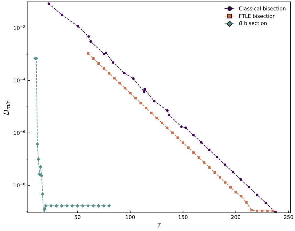
A direct mutual comparison of the local methods suggests that FTLE-based edge tracking requires time horizons one order of magnitude larger than the LD-based edge tracking to achieve equivalent . Fig. 11(a) also illustrates the bottom value reached by . This can be understood as follows: FTLEs, unlike LDs, do not display any ridge near hyperbolic saddle points if the dynamics is governed by a linear system Haller 2011; Lopesino et al. 2017. As a consequence, the trajectory in the neighbourhood of the saddle point must “feel” nonlinear effects for FTLEs to be able to identify the edge as a LCS. This implies that longer times are needed for the bisection based on FTLEs compared to that based on LDs. Similarly convergence is expected to be faster in the LD case, at least when the edge state corresponds to a fixed point. Longer times can be requested in cases with more complex attractors, although this demands a more systematic investigation.
The convergence properties of these two LCS-based edge tracking algorithms in higher dimension are expected to proceed along the same lines because of the strong scalability properties of the diagnostics themselves. In the case of LDs, the function is computed directly along the trajectories, without using the Jacobian operator . The function is hence trivially generalised to arbitrary dimension according to (8), as demonstrated in (20). The full computation of all FTLEs, on the other hand, becomes unfeasible in higher dimension since is of prohibitive size , as pointed out in Babaee et al. 2017. The computation of OTD modes, with , can however grant access to the leading FTLEs at a cost Babaee et al. 2017. For =1 this amounts to , the computation of the largest FTLE is hence based on a scalable algorithm as well.
V Conclusion, discussion and outlooks
Motivated by the physical problem of subcritical laminar-turbulent transition to turbulence in hydrodynamics, we have investigated the established notion of edge manifold which charts the state space into different basins of attraction Eckhardt et al. 2007. The main contribution of this study is the recognition of stable manifolds of edge states in autonomous systems of arbitrarily high dimensions as Lagrangian Coherent Structures (LCSs). The edge manifold divides the state space in the same way as a hyperbolic repelling Lagrangian Coherent Structure, and hence a direct relation between LCS and exact coherent states can be established. The same mathematical toolbox used to highlight an LCS can then be used to highlight the edge manifold, no matter how high the dimension of the underlying state space. The price to pay for this generalisation is that only forward-time operators can be considered, which prevents one from considering attracting LCS sets such as unstable manifolds. An illustration based on two LCS diagnostics, Finite-time Lyapunov exponents (FTLEs) Haller 2015 and forward-time Lagrangian Descriptors (LDs) Mancho et al. 2013, has revealed the edge manifold in several autonomous dynamical systems of increasing dimension and complexity. By order of dimension, these models are: i) a didactic bistable two-dimensional model with only fixed points Dauchot and Manneville 1997, ii) a bistable six-dimensional model where the edge state is an unstable periodic orbit and turbulence corresponds to a stable periodic orbit Mariotti 2011, iii) a nine-dimensional model where the edge state is a periodic orbit and turbulence is represented by a chaotic saddle Moehlis et al. 2004, and eventually iv) well-resolved Navier-Stokes simulations of a periodic cell of plane Couette flow, understood as a -dimensional dynamical system Kawahara 2005. For all these models both LCS diagnostics display steep variations at the location of the edge manifold, which can be monitored using a single scalar quantity. Our findings indicate that having some prior knowledge of the system is helpful to properly identify the edge as an LCS, and that LDs are particularly sensitive to this. Approaching a model with unknown dynamical characteristics should be done in the following way: (1) the LCS diagnostic should be applied for the parameter region of interest (2) regions on both sides of a ridge in the FTLE or the boundaries between smooth or speckled regions of should be systematically explored. After testing different values of , our exploration suggests that the edge manifold emerges already for but stands out more dramatically for longer time horizons, a feature worth a more quantitative study.
Furthermore the same toolbox allows, when it is unknown, to identify the edge state (the relative attractor on the edge manifold) using iterative bisection algorithms based on the LCS diagnostics, i.e. local measures in state space rather than global considerations as in previous works. The associated algorithms have been tested on the Dauchot-Manneville model in two dimensions using both FTLEs and LDs: both outperformed the classical approaches, with a strong advantage for the LD-based methods in cases where the edge state is a fixed, point both in terms of scalability and computational cost. However, edge states are generally not fixed points.
As pointed out in Hadjighasem et al. 2017 LDs, are not objective and their connection to LCS is unclear. This has lead to some controversy regarding the interpretation of the LD maps Ruiz-Herrera 2015; Ruiz-Herrera 2016; Lopesino et al. 2017. A hitherto unreported drawback of LDs, worth a more systematic characterisation, is that their ability to highlight the edge manifold depends on the dynamical nature of the invariant sets of the system. Consequently, their low computational cost comes with uncertainty about how to interpret the plots in an system where the nature of the attractors is unknown. The FTLEs represent a computationally more expensive tool. They have a solid mathematical background, are objective diagnostics Hadjighasem et al. 2017 and with additional constraints can be precisely connected to hyperbolic LCSs Haller 2015. Furthermore, they have a more direct interpretation in terms of material barriers.
The objectivity of the FTLEs makes them independent of the frame of reference, displaying the same values on the ridges and highlighting the edge as an LCS independently of the chosen frame. LDs are not objective and changing the frame of reference would imply a change in the values of the LD maps and even their nature. A relevant example is that of an edge state consisting of a travelling wave (TW) in physical space. Choosing a fixed frame of reference would yield a different result for the LD landscape than considering a frame moving with the velocity of the TW.
The present work paves the road for the design of effective local manifold tracking methods which do not rely on measurable global properties. The local edge tracking algorithms do not rely on a Boolean approach, but can be defined as optimisers of a scalar observable. We point out that the identification of local edge properties is not limited to bistable systems, and therefore as future work a revisit of manifold-tracking methods in different situations such as Lebovitz 2012; Zammert and Eckhardt 2019; Beneitez et al. 2019 using this new framework is strongly encouraged.
Acknowledgements.
Financial support by the Swedish Research Council (VR) grant no. 2016-03541 is gratefully acknowledged. The authors thank H. Babaee for sharing the codes from Ref. Babaee et al. 2017 and for useful discussions. The late B. Eckhardt as well as P. Negi are acknowledged for useful discussions. Computing time provided by the Swedish National Infrastructure for Computing (SNIC) is gratefully acknowledged. The open source projects Julia, Python, Matplotlib and ParaView have been used for this work.References
- Nusse and Yorke (1996) H. E. Nusse and J. A. Yorke, Basins of attraction, Science 271, 1376 (1996).
- Lucarini and Bódai (2017) V. Lucarini and T. Bódai, Edge states in the climate system: exploring global instabilities and critical transitions, Nonlinearity 30, R32 (2017).
- Junginger and Hernandez (2016) A. Junginger and R. Hernandez, Lagrangian Descriptors in dissipative systems, Phys. Chem. Chem. Phys. 18, 30282 (2016).
- Sieber et al. (2014) J. Sieber, O. Omel’chenko, and M. Wolfrum, Controlling unstable chaos: stabilizing chimera states by feedback, Phys. Rev. Lett. 112, 054102 (2014).
- Rincon et al. (2007) F. Rincon, G. Ogilvie, and M. Proctor, Self-sustaining nonlinear dynamo process in Keplerian shear flows, Phys. Rev. Lett. 98, 254502 (2007).
- Marquardt et al. (2006) F. Marquardt, J. Harris, and S. M. Girvin, Dynamical multistability induced by radiation pressure in high-finesse micromechanical optical cavities, Phys. Rev. Lett. 96, 103901 (2006).
- Cassak et al. (2007) P. Cassak, J. Drake, M. Shay, and B. Eckhardt, Onset of fast magnetic reconnection, Phys. Rev. Lett. 98, 215001 (2007).
- Nave Jr and Ross (2019) G. K. Nave Jr and S. D. Ross, Global phase space structures in a model of passive descent, Commun. Nonlinear Sci. 77, 54 (2019).
- Muñoz et al. (2012) P. R. Muñoz, J. J. Barroso, A. C.-L. Chian, and E. L. Rempel, Edge state and crisis in the Pierce diode, Chaos 22, 033120 (2012).
- Chian et al. (2013) A. C.-L. Chian, P. R. Muñoz, and E. L. Rempel, Edge of chaos and genesis of turbulence, Phys. Rev. E 88, 052910 (2013).
- Reynolds (1883) O. Reynolds, An experimental investigation of the circumstances which determine whether the motion of water shall be direct or sinuous, and of the law of resistance in parallel channels, P. R. Soc. London 35, 84 (1883).
- Schmid and Henningson (2001) P. J. Schmid and D. S. Henningson, Stability and Transition in Shear Flows (Springer, 2001).
- Eckhardt et al. (2007) B. Eckhardt, T. M. Schneider, B. Hof, and J. Westerweel, Turbulence transition in pipe flow, Annu. Rev. Fluid Mech. 39, 447 (2007).
- Daviaud et al. (1992) F. Daviaud, J. Hegseth, and P. Bergé, Subcritical transition to turbulence in plane Couette flow, Phys. Rev. Lett. 69, 2511 (1992).
- Cros and Le Gal (2002) A. Cros and P. Le Gal, Spatiotemporal intermittency in the torsional Couette flow between a rotating and a stationary disk, Phys. Fluids 14, 3755 (2002).
- Kreilos et al. (2016a) T. Kreilos, T. Khapko, P. Schlatter, Y. Duguet, D. S. Henningson, and B. Eckhardt, Bypass transition and spot nucleation in boundary layers, Phys. Rev. Fluids 1, 043602 (2016a).
- Schneider and Eckhardt (2006) T. M. Schneider and B. Eckhardt, Edge of chaos in pipe flow, Chaos 16, 041103 (2006).
- Skufca et al. (2006) J. D. Skufca, J. A. Yorke, and B. Eckhardt, Edge of Chaos in a Parallel Shear Flow, Phys. Rev. Lett. 96 (2006).
- Schneider and Eckhardt (2008) T. M. Schneider and B. Eckhardt, Edge states intermediate between laminar and turbulent dynamics in pipe flow, Philos. T. R. Soc. A 367, 577 (2008).
- Duguet et al. (2008) Y. Duguet, A. P. Willis, and R. R. Kerswell, Transition in pipe flow: the saddle structure on the boundary of turbulence, J. Fluid Mech. 613, 255 (2008).
- Itano and Toh (2001) T. Itano and S. Toh, The dynamics of bursting process in wall turbulence, J. Phys. Soc. Jpn 70, 703 (2001).
- Toh and Itano (2003) S. Toh and T. Itano, A periodic-like solution in channel flow, J. Fluid Mech. 481, 67 (2003).
- Gibson et al. (2008) J. F. Gibson, J. Halcrow, and P. Cvitanović, Visualizing the geometry of state space in plane Couette flow, J. Fluid Mech. 611, 107 (2008).
- Lebovitz (2012) N. R. Lebovitz, Boundary collapse in models of shear-flow transition, Commun. Nonlinear Sci. 17, 2095 (2012).
- Moehlis et al. (2004) J. Moehlis, H. Faisst, and B. Eckhardt, A low-dimensional model for turbulent shear flows, New J. Phys. 6 (2004).
- Alligood et al. (1996) K. T. Alligood, T. D. Sauer, and J. A. Yorke, Chaos (Springer, 1996).
- Grebogi et al. (1987) C. Grebogi, E. Ott, and J. A. Yorke, Basin boundary metamorphoses: changes in accessible boundary orbits, Nucl. Phys. B-Proc. Sup. 2, 281 (1987).
- Nusse and Yorke (1989) H. E. Nusse and J. A. Yorke, A procedure for finding numerical trajectories on chaotic saddles, Physica D 36, 137 (1989).
- Sweet et al. (2001) D. Sweet, H. E. Nusse, and J. A. Yorke, Stagger-and-step method: Detecting and computing chaotic saddles in higher dimensions, Phys. Rev. Lett. 86, 2261 (2001).
- Bollt (2005) E. M. Bollt, The path towards a longer life: On invariant sets and the escape time landscape, Int. J. Bifurcat. Chaos 15, 1615 (2005).
- Beneitez et al. (2019) M. Beneitez, Y. Duguet, P. Schlatter, and D. S. Henningson, Edge tracking in spatially developing boundary layer flows, J. Fluid Mech. 881, 164 (2019).
- Khapko et al. (2014) T. Khapko, Y. Duguet, T. Kreilos, P. Schlatter, B. Eckhardt, and D. S. Henningson, Complexity of localised coherent structures in a boundary-layer flow, Eur. Phys. J. E 37, 32 (2014).
- Duguet et al. (2013) Y. Duguet, A. Monokrousos, L. Brandt, and D. S. Henningson, Minimal transition thresholds in plane Couette flow, Phys. Fluids 25, 084103 (2013).
- Kerswell (2018) R. Kerswell, Nonlinear Nonmodal Stability Theory, Annu. Rev. Fluid Mech. 50, 319 (2018).
- Kreilos and Eckhardt (2012) T. Kreilos and B. Eckhardt, Periodic orbits near onset of chaos in plane Couette flow, Chaos 22, 047505 (2012).
- Avila et al. (2013) M. Avila, F. Mellibovsky, N. Roland, and B. Hof, Streamwise-localized solutions at the onset of turbulence in pipe flow, Phys. Rev. Lett. 110, 224502 (2013).
- Zammert and Eckhardt (2015) S. Zammert and B. Eckhardt, Crisis bifurcations in plane Poiseuille flow, Phys. Rev. E 91, 041003 (2015).
- Haller (2015) G. Haller, Lagrangian Coherent Structures, Annu. Rev. Fluid Mech. 47, 137 (2015).
- Haller and Yuan (2000) G. Haller and G. Yuan, Lagrangian coherent structures and mixing in two-dimensional turbulence, Physica D 147, 352 (2000).
- Peacock and Haller (2013) T. Peacock and G. Haller, Lagrangian coherent structures: The hidden skeleton of fluid flows, Phys. Today 66, 41 (2013).
- Aldridge (2006) B. Aldridge, Direct Lyapunov exponent analysis enables parametric study of transient signalling governing cell behaviour, IEE P. Syst. Biol. 153, 425 (2006).
- Mancho et al. (2013) A. M. Mancho, S. Wiggins, J. Curbelo, and C. Mendoza, Lagrangian descriptors: A method for revealing phase space structures of general time dependent dynamical systems, Commun. Nonlinear Sci. 18, 3530 (2013).
- Mendoza et al. (2014) C. Mendoza, A. Mancho, and S. Wiggins, Lagrangian descriptors and the assessment of the predictive capacity of oceanic data sets, Nonlin. Proc. Geoph. 21, 677 (2014).
- Haller (2011) G. Haller, A variational theory of hyperbolic Lagrangian Coherent Structures, Physica D 240, 574 (2011).
- Hadjighasem et al. (2017) A. Hadjighasem, M. Farazmand, D. Blazevski, G. Froyland, and G. Haller, A critical comparison of Lagrangian methods for coherent structure detection, Chaos 27, 053104 (2017).
- Haller and Sapsis (2011) G. Haller and T. Sapsis, Lagrangian coherent structures and the smallest finite-time Lyapunov exponent, Chaos 21, 023115 (2011).
- Babaee and Sapsis (2016) H. Babaee and T. P. Sapsis, A minimization principle for the description of modes associated with finite-time instabilities, P. R. Soc. A 472, 20150779 (2016).
- Babaee et al. (2017) H. Babaee, M. Farazmand, G. Haller, and T. P. Sapsis, Reduced-order description of transient instabilities and computation of finite-time Lyapunov exponents, Chaos 27, 063103 (2017).
- Mendoza and Mancho (2010) C. Mendoza and A. M. Mancho, Hidden geometry of ocean flows, Phys. Rev. Lett. 105, 038501 (2010).
- Lopesino et al. (2017) C. Lopesino, F. Balibrea-Iniesta, V. J. García-Garrido, S. Wiggins, and A. M. Mancho, A theoretical framework for Lagrangian Descriptors, Int. J. Bifurcat. Chaos 27, 1730001 (2017).
- Naik and Wiggins (2019) S. Naik and S. Wiggins, Finding normally hyperbolic invariant manifolds in two and three degrees of freedom with Hénon-Heiles-type potential, Phys. Rev. E 100, 022204 (2019).
- Naik et al. (2019) S. Naik, V. J. García-Garrido, and S. Wiggins, Finding NHIM: Identifying high dimensional phase space structures in reaction dynamics using Lagrangian descriptors, Commun. Nonlinear Sci. 79, 104907 (2019).
- Allshouse and Peacock (2015) M. R. Allshouse and T. Peacock, Lagrangian based methods for coherent structure detection, Chaos 25, 097617 (2015).
- Lorenz (1963) E. N. Lorenz, Deterministic Nonperiodic Flow, J. Atmos. Sci. 20, 130 (1963).
- Waleffe (1997) F. Waleffe, On a self-sustaining process in shear flows, Phys. Fluids 9, 883 (1997).
- Dauchot and Manneville (1997) O. Dauchot and P. Manneville, Local Versus Global Concepts in Hydrodynamic Stability Theory, J. Phys. II 7, 371 (1997).
- Strogatz (2001) S. Strogatz, Nonlinear Dynamics And Chaos: With Applications To Physics, Biology, Chemistry, And Engineering (Studies in Nonlinearity) (Westview Press, 2001).
- Lebovitz and Mariotti (2013) N. Lebovitz and G. Mariotti, Edges in models of shear flow, J. Fluid Mech. 721, 386 (2013).
- Hof et al. (2006) B. Hof, J. Westerweel, T. M. Schneider, and B. Eckhardt, Finite lifetime of turbulence in shear flows, Nature 443, 59 (2006).
- Mariotti (2011) G. Mariotti, A low dimensional model for shear turbulence in plane poiseuille flow: an example to understand the edge, In Proceedings of the Program in Geophysical Fluid Dynamics (2011).
- (61) The parameters , and are functions of the wavenumbers and , determined from the formulas in Mariotti 2011. The values of taken here are . The parameter is akin to the Reynolds number in fluid mechanics and chosen to be .
- Tél and Lai (2008) T. Tél and Y.-C. Lai, Chaotic transients in spatially extended systems, Phys. Rep. 460, 245 (2008).
- Schmiegel and Eckhardt (1997) A. Schmiegel and B. Eckhardt, Fractal stability border in plane Couette flow, Phys. Rev. Lett. 79, 5250 (1997).
- (64) The size of the domain is chosen to be and , fixing the wavenumbers of the Fourier modes of the model.
- Kawahara and Kida (2001) G. Kawahara and S. Kida, Periodic motion embedded in plane Couette turbulence: regeneration cycle and burst, J. Fluid Mech. 449, 291 (2001).
- (66) Numerical simulation of the Couette system is performed using the well-tested in-house unsteady spectral code SIMSON Chevalier et al. 2007. Periodic boundary conditions are imposed in the and directions, while Dirichlet boundary conditions apply at the walls at 1. The resolution used is the same as in Kawahara and Kida 2001, where a very similar spectral decomposition is used.
- Kawahara (2005) G. Kawahara, Laminarization of minimal plane Couette flow: going beyond the basin of attraction of turbulence, Phys. Fluids 17, 041702 (2005).
- Chantry and Schneider (2014) M. Chantry and T. M. Schneider, Studying edge geometry in transiently turbulent shear flows, J. Fluid Mech. 747, 506 (2014).
- Feppon and Lermusiaux (2019) F. Feppon and P. F. Lermusiaux, The extrinsic geometry of dynamical systems tracking nonlinear matrix projections, SIAM J. Matrix Anal. A. 40, 814 (2019).
- Cossu et al. (2010) C. Cossu, M. Chevalier, and D. S. Henningson, Secondary optimal growth and subcritical transition in the plane Poiseuille flow, in Seventh IUTAM Symposium on Laminar-Turbulent Transition (Springer, 2010) pp. 129–134.
- Khapko et al. (2016) T. Khapko, T. Kreilos, P. Schlatter, Y. Duguet, B. Eckhardt, and D. S. Henningson, Edge states as mediators of bypass transition in boundary-layer flows, J. Fluid Mech. 801, R2 (2016).
- Kreilos et al. (2016b) T. Kreilos, T. Khapko, P. Schlatter, Y. Duguet, D. S. Henningson, and B. Eckhardt, Bypass transition and spot nucleation in boundary layers, Phys. Rev. Fluids 1, 043602 (2016b).
- Zammert and Eckhardt (2019) S. Zammert and B. Eckhardt, Transition to turbulence when the Tollmien–Schlichting and bypass routes coexist, J. Fluid Mech. 880, R2 (2019).
- Canton et al. (2020) J. Canton, E. Rinaldi, R. Örlü, and P. Schlatter, Critical Point for Bifurcation Cascades and Featureless Turbulence, Phys. Rev. Lett. 124, 014501 (2020).
- Ruiz-Herrera (2015) A. Ruiz-Herrera, Some examples related to the method of Lagrangian descriptors, Chaos 25, 063112 (2015).
- Ruiz-Herrera (2016) A. Ruiz-Herrera, Performance of Lagrangian descriptors and their variants in incompressible flows, Chaos 26, 103116 (2016).
- Chevalier et al. (2007) M. Chevalier, P. Schlatter, A. Lundbladh, and D. S. Henningson, SIMSON - A pseudo-spectral solver for incompressible boundary layer flows, Tech. Rep. (KTH Royal Institute of Technology, 2007).