Local gravity test of unified models of inflation and dark energy
in $f(R)$ gravity

Mai Yashiki Email: g005wb@yamaguchi-u.ac.jp Affiliation: Graduate School of Sciences and Technology for Innovation, Yamaguchi University, Yamaguchi 753-8512, Japan Nobuyuki Sakai Email: nsakai@yamaguchi-u.ac.jp Affiliation: Graduate School of Sciences and Technology for Innovation, Yamaguchi University, Yamaguchi 753-8512, Japan Ryo Saito Email: rsaito@yamaguchi-u.ac.jp Affiliation: Graduate School of Sciences and Technology for Innovation, Yamaguchi University, Yamaguchi 753-8512, Japan

August 11, 2026

Abstract

We consider $f(R)$ gravity theories which unify $R^{n}$ inflation and dark energy models. First, from the final Planck data of the cosmic microwave background, we obtain a condition, $1.977<n<2.003$ . Next, under this constraint, we investigate local-gravity tests for three models. We find that the $R^{n}$ term can dominate over the dark energy term even at the Earth’s curvature scale, contrary to intuition; however, the $R^{n}$ term does not relax or tighten the constraints on the three models.

pacs

Valid PACS appear here

I Introduction

There have been growing evidences that the Universe experiences two accelerated expansion eras: inflation guth; sato; planck2018_X and the late-time acceleration 1a; 1a2; 1a3. However, in spite of many attempts, the origin(s) of both cosmic accelerations has/have not been identified yet.

Both for inflation and the late-time acceleration, models are classified into two categories: dark energy (DE) and modified gravity (MG). In the first approach, one introduces exotic matter components such as the cosmological constant or a scalar field, which is called DE for the late-time acceleration. If the exotic component has an equation of state with $w\equiv P/\rho<-1/3$ , it drives the accelerated expansion of the Universe. The other approach is to modify the theory of gravity from general relativity (GR) mog; mog2; mog3. A simple family of the modified gravity is $f(R)$ theories barrow; maeda, where the Ricci scalar $R$ in the Einstein-Hilbert action is replaced by a nonlinear function $f(R)$ . In $f(R)$ gravity, by choosing an appropriate function $f(R)$ , the expansion of the Universe is accelerated without introducing any exotic matter components.

An example of an inflationary model in $f(R)$ theories is the Starobinsky model $f(R)=R+\alpha R^{2}$ tomita; r^2. The Starobinsky model is known as the first inflationary model and its prediction gives a good fit to the Planck data for the spectral index $n_{s}$ and the tensor-to-scalar ratio $r$ inf_bestmodel; planck2018_X. On the other hand, it is known that some other forms of $f(R)$ can drive the late-time acceleration fr-DE; plmodel; fr-grav; AB-Do.

On this ground, it has been considered whether a single $f(R)$ model can describe both the early and late accelerated expansion eras in a unified way ABS; 0608008; unif_model; lalak. Such unified models should not only be viable as a model for the two accelerations but also satisfy a local-gravity test. In $f(R)$ theories, the law of gravity in a local system is modified as well as that on cosmological scales. In more words, there is an extra scalar degree of freedom with a universal coupling to matter, which is called scalaron r^2. Therefore, it mediates a fifth force and can violate local-gravity constraints. A possible resolution for this problem is given by the chameleon screening mechanism chameleon; chameleon2, which makes the range of the fifth force short in high-density regions and an $f(R)$ model compatible with the local-gravity constraints. In fact, for some $f(R)$ models of the late-time acceleration HuSawicki; StaDE, the chameleon screening mechanism is known to work without spoiling their success in cosmology.

In this paper we consider a class of $f(R)$ unified models:

f(R)=R+\alpha R^{n}+f_{\rm DE}(R)\,,

(1)

and give local-gravity constraints on three concrete models. In previous studies lalak; 0707.1941; 0710.1738; 0712.4017; 1012.2280 there have been several discussions related to this subject. Artymowski and Lalak lalak studied the model of $f_{\rm DE}(R)=-\beta R^{2-n}$ and claimed that their unified model is consistent with local-gravity tests due to the existence of $\alpha R^{n}$ term (hereafter, the $\alpha$ term), though they did not give any concrete analysis on the fifth force. One of our motivations is to verify their conclusion.

Nojiri et al. 0707.1941; 0712.4017; 1012.2280 studied some unified models where the inflation term approaches constant as $R$ goes to infinity, which is a different class of models from (1). Nojiri and Odintsov 0710.1738 also investigated a model of $f(R)=R+(\alpha R^{2n}-\beta R^{n})/(1+\gamma R^{n})$ . This model does not fall into the class (1) in a strict sense; however, their inflationary term approaches $\propto R^{n}$ as $R$ becomes large enough. In this sense our work is an extension of Ref. 0710.1738.

In the local-gravity analysis, we newly investigate two points: (i) how important the inflationary term can be and (ii) the full analysis of the fifth force taking into account the chameleon screening mechanism in the unified models. In the above models lalak; 0710.1738, the inflationary and DE terms are related and hence it is difficult to discuss how the inflationary term affects the local-gravity analysis. To avoid this subtlety, we consider three unified models where the model parameters in the inflationary and DE terms are independent. One may think intuitively that the inflationary term is negligible in local-gravity analysis. However, we find that the inflationary term can dominate over the DE term even at the Earth’s curvature scale, depending on model parameters. We therefore stress that the inflationary term should also be taken into account to estimate the fifth force and to give constraints models from local-gravity tests. Then, we give the full analysis of the fifth force in the unified models without dropping the inflationary term. The scalaron’s mass has been estimated in the literature but we also estimate the scalar charge, or the thin-shell parameter, of a gravitational object. To determine the scalar charge, one needs to know the global field profile of the scalaron from the inner region to the outer region of the object, where the curvature scale varies from the astrophysical scale to the cosmological scale. Therefore, both of the inflationary and DE terms can be relevant in this analysis.

The unified models should consistently describe the evolution of the Universe from inflation to the current accelerated expansion. Therefore, the model parameters in the inflationary term should be constrained from the inflationary era, i.e. the constraints from the primordial spectral index $n_{s}$ and the tensor-to-scalar ratio $r$ . Then, under this constraint, we analyze the chameleon screening mechanism with the inflationary term for the three unified models.

This paper is organized as follows. First, in Sec. II, we show basic equations of $f(R)$ theories used in this paper. In Sec. III, we introduce the unified models and their corresponding form in the Einstein frame. In Sec. IV, the inflationary constraints are derived for the unified models, which is extended from our previous paper my1st. In Sec. V, the local-gravity test is studied for the unified models. Finally, Sec. VI is devoted to the conclusion.

In the following, we set $8\pi G\equiv M_{\rm pl}^{-2}=1$ , where $G$ is the gravitational constant and $M_{\rm pl}$ is the reduced Planck mass.

II Basic equations

To begin with, let us briefly show some basic equations of a general $f(R)$ model used in this paper. (See, e.g., Ref. fr-grav for a more extensive review.)

The action of $f(R)$ gravity is given by

{\cal S}=\frac{1}{2}\int d^{4}x\sqrt{-g}f(R)+\int d^{4}x\sqrt{-g}{\cal L}_{\rm m}(g_{\mu\nu},\Phi_{\rm m}),

(2)

where ${\cal L}_{\rm m}$ is a matter Lagrangian density and a matter field $\Phi_{m}$ is assumed to minimally couple to the metric $g_{\mu\nu}$ .

Varying Eq. (2) with respect to $g_{\mu\nu}$ , we obtain

	$\displaystyle F(R)R_{\mu\nu}(g)$	$\displaystyle-$	$\displaystyle\frac{1}{2}f(R)g_{\mu\nu}-\nabla_{\mu}\nabla_{\nu}F(R)$		(3)
		$\displaystyle+$	$\displaystyle g_{\mu\nu}\Box F(R)=T^{({\rm m})}_{\mu\nu},$		(3)

where $F(R)\equiv{\rm d}f/{\rm d}R$ and $T^{({\rm m})}_{\mu\nu}$ is the energy-momentum tensor of the matter field. The trace of Eq. (3) gives

3\Box F+FR-2f=T^{({\rm m})},

(4)

where $T^{({\rm m})}\equiv g^{\mu\nu}T^{({\rm m})}_{\mu\nu}$ . This propagating degree of freedom $F$ corresponds to the scalaron, which is absent in general relativity because it corresponds to $F=1$ .

It is sometimes more intuitive to use the Einstein frame action as follows e-frame; e-frame2. The action (2) can be rewritten as

{\cal S}=\int d^{4}x\sqrt{-g}\left(\frac{1}{2}FR-U(F)\right)+\int d^{4}x{\cal L}_{\rm m}(g_{\mu\nu},\Phi_{\rm m}),

(5)

where $U(F)$ is defined by

U(F)=\frac{FR-f}{2}.

(6)

To obtain the action in the Einstein frame, we make the conformal transformation e-frame; maeda,

\tilde{g}_{\mu\nu}=Fg_{\mu\nu},

(7)

where a tilde denotes a quantity in the Einstein frame. Here, we introduce a scalar field $\phi$ by

\phi\equiv\sqrt{\frac{3}{2}}\ln{F}.

(8)

Using Eqs. (7) and (8), the action (5) can be rewritten as

\begin{split}{\cal S}_{\rm E}&=\int d^{4}x\sqrt{-\tilde{g}}\left[\frac{1}{2}\tilde{R}-\frac{1}{2}\tilde{g}^{\mu\nu}\partial_{\mu}\phi\partial_{\nu}\phi-V(\phi)\right]\\ &\qquad+\int d^{4}x{\cal L}_{\rm m}(F^{-1}(\phi)\tilde{g}_{\mu\nu},\Phi_{\rm m}),\end{split}

(9)

where $V(\phi)$ is the field potential in the Einstein frame:

V(\phi)=\frac{U}{F^{2}}=\frac{FR-f}{2F^{2}}.

(10)

In the Einstein frame, the scalar field equation is given by

\widetilde{\square}\phi=\frac{{\rm d}V_{\rm eff}}{{\rm d}\phi}\,,

(11)

where the effective potential is defined as

V_{\rm eff}(\phi)=V(\phi)+\rho^{*}e^{-\frac{\phi}{\sqrt{6}}}\,,

(12)

for a non-relativistic object chameleon. Here, $\rho^{*}$ is a conserved quantity in the Einstein frame, which is related to the energy density $\rho$ in the Jordan frame as $\rho^{*}=e^{-3\phi/\sqrt{6}}\rho$ . In relevant cases, the difference between these two densities is negligible because $\phi\ll 1$ . Therefore, we will omit the asterisk hereafter.

III $f(R)$ unified models

We consider a class of $f(R)$ unified models (1). The $f(R)$ models should satisfy viable conditions that tachyonic and ghost instabilities are absent. The conditions can be written in terms of $F$ as

F>0\\ \ ,\hskip 14.22636ptF_{,R}\equiv{\rm d}F/{\rm d}R>0\\ \ ,\hskip 14.22636pt{\rm for}\hskip 14.22636ptR\geq R_{0},

(13)

where $R_{0}$ is the present value of the Ricci scalar. (See, e.g., Ref. fr-grav for more details on these issues.)

We consider three types of the DE terms, $f_{\rm DE}(R)$ , as follows.

III.1 Model 1: Power-law DE model

First, we introduce the following unified model:

f(R)=R+\alpha R^{n}-\beta R^{p}\,,

(14)

with $n>1$ , $0<p<1$ and $\alpha,\beta>0$ . This model is an extension of the model proposed by Artymowski and Lalak lalak, $f(R)=R+\alpha R^{n}-\beta R^{2-n}$ . For $\alpha=0$ , this model corresponds to the power-law DE model fr-DE; plmodel, which satisfies the conditions (13).

In the model (14), the field potential in the Einstein frame (10) is read as

V(\phi)=\frac{e^{-\frac{4}{\sqrt{6}}\phi}}{2}\left[\alpha(n-1)R(\phi)^{n}+\beta(1-p)R(\phi)^{p}\right]\,.

(15)

Here, $R(\phi)$ is obtained by solving the equation,

e^{\frac{2}{\sqrt{6}}\phi}=F(R)=1+\alpha nR^{n-1}-\beta pR^{p-1}\,,

(16)

which is regular when the stability conditions (13) are satisfied.

The first derivative of the field potential is

	$\displaystyle V_{,\phi}$	$\displaystyle\equiv\frac{{\rm d}V}{{\rm d}\phi}=-\frac{FR-2f}{\sqrt{6}F^{2}}$
		$\displaystyle=\frac{e^{-\frac{4}{\sqrt{6}}\phi}R}{\sqrt{6}}\left[1+\alpha(2-n)R^{n-1}-\beta(2-p)R^{p-1}\right]\,.$		(17)

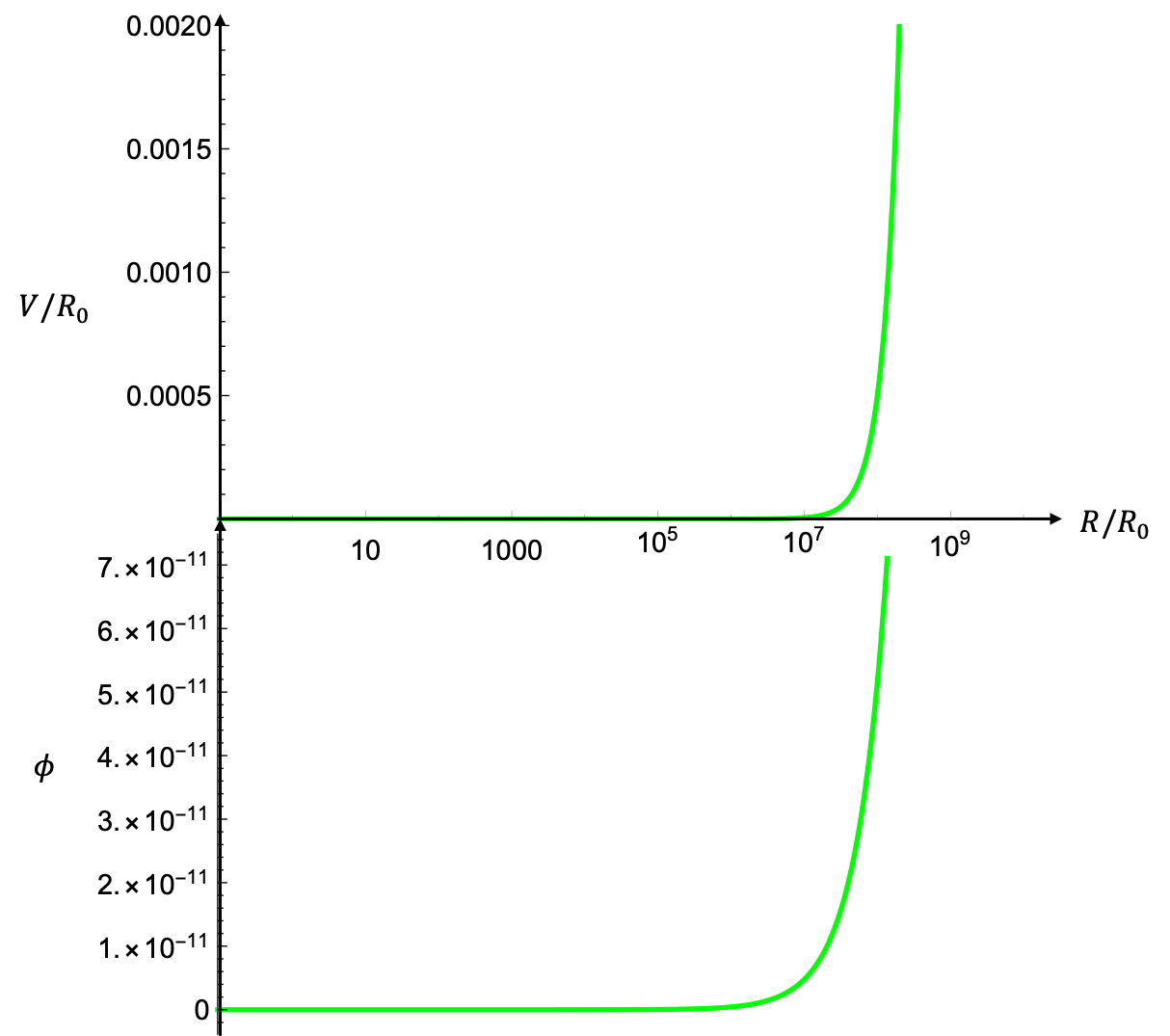
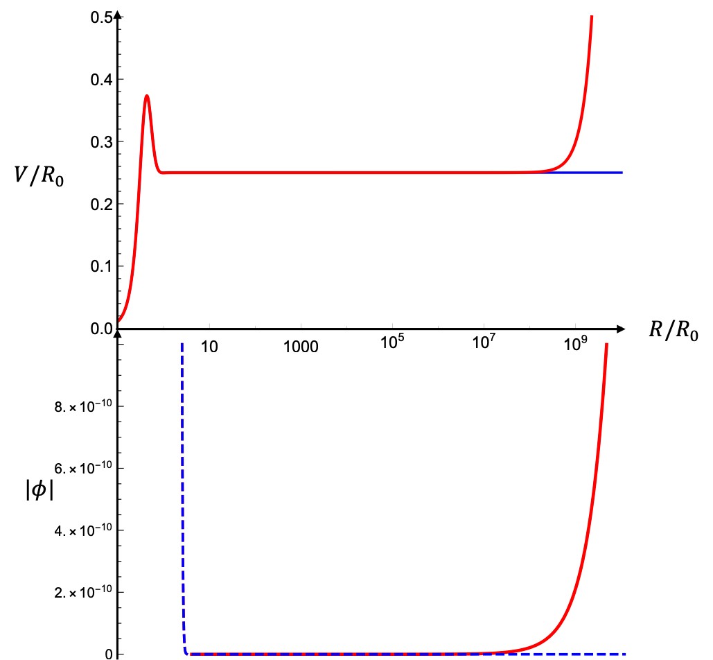
In the absence of the $\beta$ term, the field potential has a minimum $V=0$ at $R=0$ , which corresponds to $\phi=0$ (see Fig. 1). Therefore, the expansion of the Universe is not accelerated without introducing matter. In contrast, when the $\beta$ term is introduced, a minimum appears at $R=R_{\rm min}\simeq[\beta(2-p)]^{1/(1-p)}>0$ and $V>0$ at the minimum, while $R=0$ cannot be reached now because the field value $\phi$ diverges at $R=R_{F=0}\simeq[\beta p]^{1/(1-p)}>0$ (see Fig. 2). As in the original model lalak, this potential energy drives the late-time acceleration.

Refer to caption — Figure 1: Potential in the Einstein frame for $R^{2}$ inflation model. We show parametric representations $V(R)$ and $\phi(R)$ in the top and the bottom, respectively. In this model, the potential minimum is given by $V=0$ at $\phi=0$ . The potential as a function of the field value, $V(\phi)$ , is shown in Ref.fr-grav.

In the model (14), $F_{,R}$ is given by

F_{,R}=\alpha n(n-1)R^{n-2}+\beta p(1-p)R^{p-2}\,.

(18)

Thus, the second condition $F_{,R}>0$ (13) is satisfied for $n>1$ , $0<p<1$ and $\alpha,\beta>0$ . On the other hand, the first condition $F>0$ is violated for $R<R_{F=0}\simeq[\beta p]^{1/(1-p)}$ . However, the curvature $R$ never dynamically reaches to this region because there is an infinite potential barrier at $R=R_{F=0}$ .

III.2 Model 2: Starobinsky DE model

Next, we introduce the following unified model:

f(R)=R-\mu R_{\rm 0}\left[1-\left(1+\frac{R^{2}}{R^{2}_{\rm 0}}\right)^{-j}\right]+\alpha R^{n},

(19)

where $j,\mu>0$ . For $\alpha=0$ , this model corresponds to the Starobinsky DE model StaDE, which also satisfies the conditions (13). For $R\gg R_{\rm 0}$ , this model can be approximated by a power-law model as

f(R)\simeq R+\mu R_{\rm 0}\left(\frac{R}{R_{\rm 0}}\right)^{-2j}+\alpha R^{n}\,.

(20)

In the model (19), the field potential in the Einstein frame (10) and its first derivative are read as

	$\displaystyle V(\phi)=$	$\displaystyle\frac{e^{-\frac{4}{\sqrt{6}}\phi}}{2}\Bigg[\mu R_{0}+\alpha(n-1)R^{n}-\mu R_{0}$
		$\displaystyle\left.\times\left(1+\frac{R^{2}}{R_{0}^{2}}\right)^{-j}\left(1+2j\left(1+\frac{R_{0}^{2}}{R^{2}}\right)^{-1}\right)\right]\,,$		(21)

and

	$\displaystyle V_{,\phi}=$	$\displaystyle\frac{e^{-\frac{4}{\sqrt{6}}\phi}}{\sqrt{6}}\Biggl[R-2\mu R_{0}+\alpha(2-n)R^{n}$
		$\displaystyle+2\mu R_{0}\left(1+\frac{R^{2}}{R_{0}^{2}}\right)^{-j}\left(1+j\left(1+\frac{R_{0}^{2}}{R^{2}}\right)^{-1}\right)\Biggr]\,,$		(22)

where

e^{\frac{2}{\sqrt{6}}\phi}=F(R)=1+\alpha nR^{n-1}-2\mu j\frac{R}{R_{0}}\left(1+\frac{R^{2}}{R_{0}^{2}}\right)^{-j-1}\,.

(23)

In the model (19), $F_{,R}$ becomes

	$\displaystyle F_{,R}=$	$\displaystyle\alpha n(n-1)R^{n-2}-\frac{2\mu j}{R_{0}}\left(1+\frac{R^{2}}{R_{0}^{2}}\right)^{-j-1}$
		$\displaystyle\times\left[1-2\mu(j+1)\left(1+\frac{R_{0}^{2}}{R^{2}}\right)^{-1}\right]\,.$		(24)

When the DE term is introduced, a minimum appears at $R=R_{\rm min}\simeq R_{0}$ and $V>0$ at the minimum (see Fig. 3). Therefore, the potential energy drives the late-time acceleration in the model.

III.3 Model 3: $g$ -AB model

Finally, we introduce the following unified model:

f(R)=(1-g)R+g\epsilon_{\rm AB}\ln\left[\frac{\cosh(R/\epsilon_{\rm AB}-b)}{\cosh b}\right]+\alpha R^{n}\,,

(25)

where $b>0$ , $0<g<1/2$ , and

\epsilon_{\rm AB}\equiv\frac{R_{0}}{2g\ln(1+e^{2b})}\,.

(26)

This model is an extension of the model proposed by Appleby et al. ABS, where the model has $n=2$ . For $\alpha=0$ and $g=1/2$ , this model corresponds to the Appleby & Battye (AB) model AB, which also satisfies the conditions (13). The constraints on $g$ and $b$ are obtained from the stability conditions (13). We show the relation between $g$ and $b$ in Fig. 4 (see ABS for more details).

For $R\gg R_{\rm 0}$ , the model (25) can be approximated by

f(R)\simeq R-\frac{R_{0}}{2}+g\epsilon_{AB}\,e^{2b}e^{-2R/\epsilon_{AB}}+\alpha R^{n}\,.

(27)

In the model (25), the field potential in the Einstein frame (10) and the first derivative of the potential read,

	$\displaystyle V(\phi)=$	$\displaystyle\frac{e^{-\frac{4}{\sqrt{6}}\phi}}{2}\Biggl[\alpha(n-1)R^{n}+gR\tanh\left(\frac{R}{\epsilon_{\rm AB}}-b\right)$
		$\displaystyle-g\epsilon_{\rm AB}\log\left(\frac{\cosh(R/\epsilon_{\rm AB}-b)}{\cosh b}\right)\Biggr]\,,$		(28)

and

	$\displaystyle V_{,\phi}=$	$\displaystyle\frac{e^{-\frac{4}{\sqrt{6}}\phi}}{\sqrt{6}}\Biggl[R(1-g)+\alpha(2-n)R^{n}-gR\tanh\left(\frac{R}{\epsilon_{\rm AB}}-b\right)$
		$\displaystyle+2g\epsilon_{\rm AB}\log\left(\frac{\cosh(R/\epsilon_{\rm AB}-b)}{\cosh b}\right)\Biggr]\,,$		(29)

where

	$\displaystyle e^{\frac{2}{\sqrt{6}}\phi}$	$\displaystyle=F(R)$
		$\displaystyle=1-g+\alpha nR^{n-1}+g\tanh\left(\frac{R}{\epsilon_{\rm AB}}-b\right)\,.$		(30)

In the model (25), $F_{,R}$ becomes

F_{,R}=\alpha n(n-1)R^{n-2}+\frac{g}{\epsilon_{\rm AB}}\,{\rm sech}^{2}\left(\frac{R}{\epsilon_{\rm AB}}-b\right)\,.

(31)

When the DE term is introduced, a minimum appears at $R=R_{\rm min}\simeq b\epsilon_{\rm AB}>0$ and $V>0$ at the minimum (see Fig. 5).

IV Inflationary constraints

Next, we derive an inflationary constraint on the unified models. Since inflation is driven without introducing any matter in $f(R)$ theories, we neglect the matter in this section. In addition, the Ricci scalar $R$ is sufficiently large during inflation. Hence, the function $f(R)$ in all the unified models above can be approximated as

f(R)\simeq R+\alpha R^{n}\,,

(32)

which is an extension of $R^{2}$ model tomita; r^2 (see 1311.0744 another extended $R^{2}$ model). This model (32) corresponds to the Einstein frame action with

V(\phi)=V_{0}e^{-\frac{4}{\sqrt{6}}\phi}\left[e^{\frac{2}{\sqrt{6}}\phi}-1\right]^{\frac{n}{n-1}}\,,

(33)

where $V_{0}\equiv\alpha(n-1)/[2(\alpha n)^{n/(n-1)}]$ .

Since the comoving curvature perturbations and tensor perturbations are invariant under the conformal transformation (7) chiba-yamaguchi; pertub_c-t, the spectral index $n_{s}$ and the tensor-to-scalar ratio $r$ can be directly evaluated in the Einstein frame, where the action is equivalent to that in a single-field slow-roll inflationary model. Therefore, they are given as,

r=16\epsilon_{V}\,,\quad n_{s}=1-6\epsilon_{V}+2\eta_{V}\,,

(34)

in terms of the slow-roll parameters,

\epsilon_{V}\equiv\frac{1}{2}\left(\frac{V_{,\phi}}{V}\right)^{2}\,,\quad\eta_{V}\equiv\frac{V_{,\phi\phi}}{V}\,.

(35)

In the model (32), the slow-roll parameters are evaluated as Motohashi,

	$\displaystyle\epsilon_{V}$	$\displaystyle=$	$\displaystyle\frac{4E_{k}^{2}(2-n)^{2}}{3[2(n-1)E_{k}-n]^{2}},$		(36)
	$\displaystyle\eta_{V}$	$\displaystyle=$	$\displaystyle\frac{4(2-n)\left[2(2-n)E_{k}^{2}-nE_{k}+n\right]}{3[2(n-1)E_{k}-n]^{2}},$		(37)

where $E_{k}\equiv\mathrm{e}^{4(2-n)N_{k}/(3n)}$ and $N_{k}$ is e-folds from the horizon crossing to the end of inflation. They reduce to the well-known results,

\epsilon_{V}=\frac{3}{4N_{k}^{2}}\,,\quad\eta_{V}=-\frac{1}{N_{k}}\,,

(38)

in the limit $n\to 2$ .

We compare these predictions with the Planck data planck2018_X:

r<0.01,\,\,\,n_{s}=0.9659\pm 0.0041\hskip 8.53581pt(95\,\%\,{\rm CL})\,.

(39)

As a result, the index $n$ in the model (32) is constrained as

	$\displaystyle N_{k}=50:1.977<$	$\displaystyle n$	$\displaystyle<1.991\hskip 14.22636pt(95\,\%\,{\rm CL})\,,$		(40)
	$\displaystyle N_{k}=60:1.991<$	$\displaystyle n$	$\displaystyle<2.003\hskip 14.22636pt(95\,\%\,{\rm CL})\,.$		(41)

Note that this constraint is slightly relaxed from our previous result $1.965<n<2$ my1st. In the original model $f(R)=R+\alpha R^{n}-\beta R^{2-n}$ , $p$ is fixed to be $p=2-n$ . Therefore, the viable condition $0<p<1$ restricts $n$ as $1<n<2$ . In the extended model (14), this constraint is absent.

In addition, we can estimate the model parameter $\alpha$ from the amplitude of the scalar power spectrum,

{\cal P_{R}}=\frac{H_{E}^{2}}{8\pi^{2}\epsilon_{V}}\simeq\frac{N_{k}^{2}}{144\pi^{2}\alpha}\,,

(42)

where $H_{E}$ is the Hubble parameter in the Einstein frame and we used $n\simeq 2$ in the second equation. Comparing this with the CMB observation ${\cal P_{R}}\sim 10^{-10}$ planck2018_X, we find

\alpha\sim 10^{10}\,,

(43)

for $N_{k}=50\--60$ .

V local-gravity constraint

Here, we consider the local-gravity constraint on the unified models (14), (20) and (27) following the analysis in Refs. fr-DE; ABS. In this section, we work in the Einstein frame, where it is more clear that the extra degree of freedom, i.e. scalaron, mediates the fifth force as

\vec{F}_{\phi}=\frac{M}{\sqrt{6}}\vec{\nabla}\phi.

(44)

In this analysis, we study the configuration of the scalar field in the finite density region, which is governed by Eq. (11):

\widetilde{\square}\phi=\frac{{\rm d}V_{\rm eff}}{{\rm d}\phi}\,;\quad V_{\rm eff}(\phi)=V(\phi)+\rho e^{-\frac{\phi}{\sqrt{6}}}\,.

(45)

The minimum of the effective potential $\phi=\phi_{\rm min}$ depends on the density $\rho$ through

\frac{{\rm d}V_{\rm eff}}{{\rm d}\phi}=V_{,\phi}-\frac{\rho e^{-\frac{\phi_{\rm min}}{\sqrt{6}}}}{\sqrt{6}}=0\,,

(46)

and the scalaron’s mass also depends on $\rho$ through

m_{\phi}^{2}\equiv\frac{d^{2}V_{\rm eff}(\phi_{\rm min})}{d\phi^{2}}=V_{,\phi\phi}+\frac{\rho e^{-\frac{\phi_{\rm min}}{\sqrt{6}}}}{6},

(47)

at the minimum $\phi=\phi_{\rm min}$ . These imply that the range of the fifth force changes according to the density in its environment. This is known as the chameleon screening mechanism chameleon; chameleon2. In the following, we see if the unified models (14), (20) and (27) can evade the local-gravity constraint by the chameleon screening mechanism.

V.1 Chameleon screening mechanism

First, we briefly review the chameleon screening mechanism for the fifth force sourced by a star, modeling it as a spherically symmetric non-relativistic object with a constant density $\rho_{c}$ . It is assumed that the star is surrounded by baryons and dark matter with a homogeneous density $\rho_{\rm G}\simeq 10^{-24}{\rm g/cm^{3}}$ chameleon. In this analysis, we focus on the vicinity of the star and neglect the cosmic expansion.

Assuming a static and spherically symmetric profile, the field equation reduces to

\frac{d^{2}\phi}{d\tilde{r}^{2}}+\frac{2}{\tilde{r}}\frac{d\phi}{d\tilde{r}}=\frac{dV_{\rm eff}}{d\phi}\,.

(48)

In the outer region, the scalaron relaxes to the minimum $\phi_{G}\equiv\phi_{\rm min}(\rho_{G})$ as

\phi\simeq\phi_{G}+\frac{Qe^{-m_{G}\tilde{r}}}{\tilde{r}}\,,

(49)

where $m_{G}\equiv m_{\phi}(\rho_{G})$ . Here, $Q$ is the scalar charge and determined by matching to an inner solution. Inside the star, the effective potential has the minimum at $\phi_{c}\equiv\phi_{\rm min}(\rho_{c})$ with a mass $m_{c}\equiv m_{\phi}(\rho_{c})$ . When the Compton wavelength $\lambda_{c}\sim 1/m_{c}$ is much shorter than the radius of the star $\tilde{r}_{c}$ ,

\lambda_{c}\ll\tilde{r}_{c}\quad(m_{c}\tilde{r}_{c}\gg 1)\,,

(50)

the scalaron stays near $\phi=\phi_{c}$ in the inside of the star and has a thin-shell profile. In this case, the scalar charge is given by chameleon,

\frac{Q}{M_{c}}=\frac{3}{4\sqrt{6}\pi}\left(\frac{\Delta\tilde{r}_{c}}{\tilde{r}_{c}}\right)\,,

(51)

in the unit of the mass of the star $M_{c}$ . Here, the thin-shell parameter $\Delta\tilde{r}_{c}/\tilde{r}_{c}$ is given as,

\frac{\Delta\tilde{r}_{c}}{\tilde{r}_{c}}=\frac{\phi_{G}-\phi_{c}}{\sqrt{6}\Phi_{c}}\,;\quad\Phi_{c}\equiv\frac{M_{c}}{8\pi\tilde{r}_{c}}\,.

(52)

Therefore, the fifth force (44) is screened when the thin-shell parameter is small enough.

When the inflationary term is absent, the $\phi_{G}$ term is dominant and the models (14), (20) and (27) approximately give,

\displaystyle\left|\frac{\Delta\tilde{r}_{c}}{\tilde{r}_{c}}\right|\simeq\begin{cases}\frac{2\tilde{\beta}p}{\Phi_{c}}\left(\frac{\rho_{G}}{R_{0}}\right)^{p-1}&\text{Power-law model (\ref{eq:ex lalak})}\\ \frac{4\mu j}{\Phi_{c}}\left(\frac{\rho_{G}}{R_{0}}\right)^{-2j-1}&\text{Starobinsky DE model (\ref{eq:Sta unified})}\\ \frac{ge^{2b}}{\Phi_{c}}\exp\left(-\frac{2\rho_{G}}{\epsilon_{AB}}\right)&\text{$g$-AB model (\ref{eq:g-AB unified})}\end{cases}

(53)

where we have introduced the dimensionless parameter,

\tilde{\beta}\equiv\beta R_{0}^{p-1}\,.

(54)

Here, the parameters $\tilde{\beta}$ and $\mu$ are estimated to be order of unity to explain the present value of the dark energy density parameter, $\Omega_{\rm DE}\simeq 0.7$ . In addition, from Fig. 4, $b>0$ under the constraint on $g$ . From these expressions, one can see that the thin-shell parameter quickly decreases as $\rho_{G}$ increases in the latter two models but only slowly in the first model. Reflecting this fact, the power-law model is tightly constrained by local-gravity tests while the other two are viable. In Table 1, we summarize the solar-system constraints for the model parameters in these DE models capo_tsujikawa; ABS. Here, the constraint is not shown for the $g$ -AB model because the solar-system constraint does not restrict the parameter region under the stability conditions (see Fig. 4).

Table 1: The solar-system constraints on the model parameters capo_tsujikawa; ABS.

DE models	constraint
Power-law model	$p<10^{-10}$
Starobinsky DE model	$j>0.9$
$g$ -AB model	-

V.2 Constraints in the unified models

As Figs. 2-5 indicate, the inflationary term can affect the scalaron’s potential even for curvatures lower than the inflationary scale. Here, therefore, we see how the local-gravity constraints can change when the inflationary term $\alpha R^{n}$ is added. For later convenience, we make $\alpha$ dimensionless as

\tilde{\alpha}=\alpha R_{0}^{n-1}\,,

(55)

which is estimated to be ¹¹ 1 Strictly speaking, this value depends on $n$ but the deviation is irrelevant under the constraint in Sec. IV, $n-2<{\cal O}(10^{-2})$ .

\tilde{\alpha}\sim 10^{-110}\,.

(56)

from the normalization (43).

V.2.1 Model 1: Power-law DE + $R+\alpha R^{n}$ model

First, we consider the model (14):

f(R)=R+\tilde{\alpha}R_{0}\left(\frac{R}{R_{0}}\right)^{n}-\tilde{\beta}R_{0}\left(\frac{R}{R_{0}}\right)^{p}\,,

(57)

where the parameters are made dimensionless as in Eqs. (54) and (55). From Table 1, this model is tightly constrained by the solar-system observations. Here, we verify whether the inflationary term can evade this constraint.

The minimum of the effective potential in this model is determined by

\frac{R}{R_{0}}+\tilde{\alpha}(2-n)\left(\frac{R}{R_{0}}\right)^{n}-\tilde{\beta}(2-p)\left(\frac{R}{R_{0}}\right)^{p}=\frac{\rho e^{-\frac{\phi}{\sqrt{6}}}}{R_{0}}\,.

(58)

with

e^{\frac{2}{\sqrt{6}}\phi}=F(R)=1+\tilde{\alpha}n\left(\frac{R}{R_{0}}\right)^{n-1}-\tilde{\beta}p\left(\frac{R}{R_{0}}\right)^{p-1}\,.

(59)

As mentioned earlier, the coefficients are roughly estimated to be,

\tilde{\alpha}\sim 10^{-110}\,,\quad\tilde{\beta}\sim 1\,.

(60)

On the other hand, for $\rho={\cal O}(10^{-24}\--1){\rm g/cm^{3}}$ , the right-hand side is roughly estimated to be,

\frac{\rho e^{-\frac{\phi}{\sqrt{6}}}}{R_{0}}\sim 10^{4}\--10^{28}\,,

(61)

where we have used $R_{0}\simeq 12H_{0}^{2}=4\rho_{\rm crit}\sim 10^{-29}{\rm g/cm^{3}}$ . Therefore, at the minimum in the relevant region, the first term in Eq. (58) is dominant and the curvature scale is given by

\frac{R_{\rm min}}{R_{0}}\simeq\frac{\rho}{R_{0}}\sim 10^{28}\left(\frac{\rho}{1{\rm g/cm^{3}}}\right)\,.

(62)

The corresponding field value at the minimum is determined by Eq. (59). For the typical values (60) and (62), $\phi_{\rm min}\ll 1$ and hence

\frac{2\phi_{\rm min}}{\sqrt{6}}\simeq\tilde{\alpha}n\left(\frac{R_{\rm min}}{R_{0}}\right)^{n-1}-\tilde{\beta}p\left(\frac{R_{\rm min}}{R_{0}}\right)^{p-1}\,.

(63)

Therefore, the modified terms are important to determine the field value $\phi_{\rm min}$ . Among these two terms, the $\alpha$ term is negligible unless the index $p$ is extremely small,

p\ll\frac{n\tilde{\alpha}}{\tilde{\beta}}\left(\frac{R_{\rm min}}{R_{0}}\right)^{n-p}\sim 10^{-54-28p}\left(\frac{\rho}{1{\rm g/cm^{3}}}\right)^{n-p}\,,

(64)

or unless the local density is sufficiently large,

\rho\gg\left(\frac{p\tilde{\beta}}{n\tilde{\alpha}}\right)^{\frac{1}{n-p}}R_{0}\sim\left(\rho_{\inf}^{n-1}\rho_{\rm crit}^{1-p}\right)^{\frac{1}{n-p}}\,,

(65)

where $\rho_{\rm inf}$ is the energy density of inflation, $\rho_{\rm inf}\simeq R_{\rm inf}\equiv\tilde{\alpha}^{-1/(n-1)}R_{0}$ . In this case, the field value is given in terms of the density as

\frac{2\phi_{\rm min}}{\sqrt{6}}\simeq-\tilde{\beta}p\left(\frac{R_{\rm min}}{R_{0}}\right)^{p-1}\simeq-\tilde{\beta}p\left(\frac{\rho}{R_{0}}\right)^{p-1}\,.

(66)

We can find that a similar approximation can be applied to the effective mass. Under this approximation, the effective mass is estimated to be,

\displaystyle m_{\phi}^{2}\simeq R_{0}\left[\frac{1}{3p(1-p)\tilde{\beta}}\left(\frac{\rho}{R_{0}}\right)^{2-p}-\frac{5\rho}{6R_{0}}\right]\,,

(67)

For small values of $p$ , the first term gives the dominant contribution,

	$\displaystyle m_{\phi}^{2}$	$\displaystyle\simeq\frac{R_{0}}{3p(1-p)\tilde{\beta}}\left(\frac{\rho}{R_{0}}\right)^{2-p}$
		$\displaystyle\sim\frac{H_{0}^{2}}{p}\left(\frac{\rho}{\rho_{\rm crit}}\right)^{2-p}\,.$		(68)

and the thin-shell parameter is unchanged from Eq. (53). From the arguments above, we found that the $\alpha$ term is irrelevant to the local-gravity analysis under the inflationary and DE constraints. Therefore, the local-gravity constraints in the model (14) reduce to those for the DE model plmodel,

f(R)=R-\beta R^{p}\,.

(69)

In Ref. lalak, where the model with $p=2-n$ is treated, they claimed without an analysis on the fifth force that their unified model is consistent with the local-gravity tests. Contrary to this statement, the power-law unified model is not viable for the local-gravity tests.

V.2.2 Model 2: Starobinsky DE + $\alpha R^{n}$ model

The above argument also showed that, in the model (14), the inflationary term can affect the local-gravity constraints for the density,

\rho\gg\rho_{\rm th}\equiv\left(\rho_{\inf}^{n-1}\rho_{\rm crit}^{1-p}\right)^{\frac{1}{n-p}}\,,

(70)

which is higher than the density relevant to the solar-system constraints but can be much lower than the inflationary scale. This observation indicates that the inflationary term can affect the local-gravity analysis depending on the model parameters in general unified models. Next, we see how the effect of the inflationary term appears in the viable models (19) and (27).

First, we consider the model (19). In a high density region, it can be approximated by the power-law model (20):

f(R)=R+\mu R_{\rm 0}\left(\frac{R}{R_{\rm 0}}\right)^{-2j}+\tilde{\alpha}R_{0}\left(\frac{R}{R_{0}}\right)^{n}\,.

(71)

Therefore, the analysis is parallel to the model (14) with the replacements $\tilde{\beta}\to-\mu$ and $p\to-2j~(j>0.9)$ , i.e. a possible value of the index is different. Taking into this fact, the threshold density can be estimated as

\rho_{\rm th}\equiv\left(\rho_{\inf}^{n-1}\rho_{\rm crit}^{1+2j}\right)^{\frac{1}{n+2j}}\,.

(72)

This shows that the inflationary term can be important even for a very low value of the density when $j$ is large.

We estimate the effective mass,

m_{\phi}^{2}=\left.\frac{1}{6}\left(\frac{FR-6f}{F^{2}}+\frac{2}{F_{,R}}\right)\right|_{R=R_{\rm min}}

(73)

without ignoring the $\alpha$ term. The first term is dominated by the GR term and estimated to be,

\left.\frac{FR-6f}{6F^{2}}\right|_{R=R_{\rm min}}\simeq-\frac{5R_{\rm min}}{6}\simeq-\frac{5\rho}{6}\,.

(74)

The second term $1/(3F_{,R})$ is determined by the inflationary/DE terms and larger than the first term for a large value of the density. Therefore, in terms of the Compton wavelength $\lambda_{\phi}=m_{\phi}^{-1}$ , it is given by a sum of the inflationary and DE pieces as

$\displaystyle\lambda_{\phi}^{2}$	$\displaystyle\simeq 3F_{,R}$
	$\displaystyle=\frac{n(n-1)}{H_{\rm inf}^{2}}\left(\frac{\rho}{\rho_{\rm inf}}\right)^{n-2}+\frac{\mu j(2j+1)}{2H_{0}^{2}}\left(\frac{\rho}{4\rho_{\rm crit}}\right)^{-2j-2}$
	$\displaystyle\sim j^{2}H_{0}^{-2}\left(\frac{\rho}{\rho_{\rm crit}}\right)^{-2j-2}\left[1+{\cal O}(1)\left(\frac{\rho}{\rho_{\rm th}}\right)^{2j+n}\right]\,,$	(75)

where we have introduced the inflationary Hubble scale $H_{\rm inf}^{2}\equiv\rho_{\rm inf}/3$ .

This result shows that the Compton wavelength first rapidly decreases as the density increases but becomes approximately constant for $\rho>\rho_{\rm th}$ with $n\simeq 2$ (see Figs. 6 - 8). In addition, the inflationary term can dominate over the DE term at smaller scales than the Earth’s scale for $j>0.9$ . The Compton wavelength can be enhanced by the factor $(\rho/\rho_{\rm inf})^{n-2}$ for $n<2$ . However, it is not large enough under the inflationary constraint (41). Therefore, the thin-shell condition (50) is kept even when the inflationary term is added. ²² 2 On the other hand, from the viewpoint of the inflationary model, the DE term makes the scalaron’s mass light in a low dense region and fifth-force constraints relevant.

Then, let us see next how the thin-shell parameter (52) is modified. With the inflationary term, the scalar field is related to the curvature/density as

	$\displaystyle\frac{2\phi_{\rm min}}{\sqrt{6}}$	$\displaystyle\simeq\tilde{\alpha}n\left(\frac{R_{\rm min}}{R_{0}}\right)^{n-1}-2\mu j\left(\frac{R_{\rm min}}{R_{0}}\right)^{-2j-1}$
		$\displaystyle\sim\left(\frac{\rho}{\rho_{\rm crit}}\right)^{-2j-1}\left[1+{\cal O}(1)\left(\frac{\rho}{\rho_{\rm th}}\right)^{2j+n}\right]\,.$		(76)

This shows that $|\phi_{\rm min}|$ increases as $\rho$ increases for $\rho>\rho_{\rm th}$ in contrast that it decreases when the inflationary term is absent. Hence, the $\phi_{c}$ term can be also important in Eq. (52).

In analyzing the thin-shell parameter (52) from the field value (76), there are three possibilities: (i) the DE term dominates over all regions $\rho_{\rm th}>\rho_{c}$ , (ii) the inflationary term dominates over all regions $\rho_{\rm th}<\rho_{G}$ , and (iii) the inflationary term dominates in the inner region of the object while the DE term does in the outer region $\rho_{G}<\rho_{\rm th}<\rho_{c}$ . In the first case, the analysis reduces to that for the DE model. In the second case, the scalaron is also heavy in the outer region and hence it is not necessary to discuss the screening mechanism. Therefore, the relevant case is $\rho_{G}<\rho_{\rm th}<\rho_{c}$ . In this case, the thin-shell parameter is estimated to be

\displaystyle\left|\frac{\Delta\tilde{r}_{c}}{\tilde{r}_{c}}\right|\simeq\frac{2}{\Phi_{c}}\left[2\mu j\left(\frac{\rho_{G}}{R_{0}}\right)^{-2j-1}+\tilde{\alpha}n\left(\frac{\rho_{c}}{R_{0}}\right)^{n-1}\right]\,,

(77)

where now the $\rho_{c}$ -dependent term can be non-negligible. The additional term is roughly estimated to be

\displaystyle\frac{2\tilde{\alpha}n}{\Phi_{c}}\left(\frac{\rho_{c}}{R_{0}}\right)^{n-1}\sim\frac{1}{\Phi_{c}}\left(\frac{\rho_{c}}{\rho_{\rm inf}}\right)^{n-1}\sim\frac{1}{H_{\rm inf}^{2}\tilde{r}_{c}^{2}}\left(\frac{\rho_{c}}{\rho_{\rm inf}}\right)^{n-2}\,,

(78)

where we have estimated the gravitational potential as $\Phi_{c}\sim\rho_{c}\tilde{r}_{c}^{2}$ . For a fixed size of the object $\tilde{r}_{c}$ , the parameter can be enhanced by the factor $(\rho_{c}/\rho_{\rm inf})^{n-2}$ for $n<2$ . However, it is not large enough under the inflationary constraint (41).

V.2.3 Model 3: $gR^{n}$ -AB model

Finally, we consider the model (25). In a high density region, it can be approximated by the exponential model (27)

f(R)\simeq R-\frac{R_{0}}{2}+g\epsilon_{AB}\,e^{2b}e^{-2R/\epsilon_{AB}}+\tilde{\alpha}R_{0}\left(\frac{R}{R_{0}}\right)^{n}\,.

(79)

As in the other models, the curvature scale at the potential minimum can be estimated as

\frac{R_{\rm min}}{R_{0}}\simeq\frac{\rho}{R_{0}}\,.

(80)

The corresponding field value is

	$\displaystyle\frac{2\phi_{\rm min}}{\sqrt{6}}$	$\displaystyle\simeq\tilde{\alpha}n\left(\frac{R_{\rm min}}{R_{0}}\right)^{n-1}-2ge^{2b}e^{-2R_{\rm min}/\epsilon_{AB}}$
		$\displaystyle=n\left(\frac{\rho}{\rho_{\rm inf}}\right)^{n-1}-2ge^{2b}e^{-2\rho/\epsilon_{AB}}\,,$		(81)

and the Compton wavelength is

\displaystyle\lambda_{\phi}^{2}\simeq\frac{n(n-1)}{H_{\rm inf}^{2}}\left(\frac{\rho}{\rho_{\rm inf}}\right)^{n-2}+\frac{2g^{2}e^{2b}\ln(1+e^{2b})}{H_{0}^{2}}e^{-2\rho/\epsilon_{AB}}\,.

(82)

We show the relation between the Compton wavelength $\lambda_{\phi}=m_{\phi}^{-1}$ and the density $\rho$ with $n=2$ in Figs. 9 - 12. The DE term decreases and the inflationary term becomes relevant for a lower value of the density than the other models. However, the Compton wavelength is asymptotic to the same small value as in the other models. Therefore, the thin-shell condition (50) is kept even when the inflationary term is added.

The thin-shell parameter is estimated to be

\displaystyle\left|\frac{\Delta\tilde{r}_{c}}{\tilde{r}_{c}}\right|\simeq\frac{1}{\Phi_{c}}\left[ge^{2b}\exp\left(-\frac{2\rho_{G}}{\epsilon_{AB}}\right)+2\tilde{\alpha}n\left(\frac{\rho_{c}}{R_{0}}\right)^{n-1}\right]\,.

(83)

The correction from the inflationary term never becomes large under the inflationary constraint (41).

VI Conclusion

In this paper, we studied cosmological and local-gravity tests on unified models of inflation and dark energy in $f(R)$ gravity for three unified models: the power-law DE model, the Starobinsky DE model, and the $g$ -AB DE model with the inflationary $R^{n}$ term.

From the observation of the primordial fluctuations by the Planck satellite, we have obtained a constraint on the index $n$ and found that it should close to two: $|n-2|<{\cal O}(0.01)$ . Moreover, the amplitude of the fluctuations determines the scale of the inflationary term.

Next, we studied the local-gravity test in the unified models. In contrast to a naive expectation, we found that the inflationary term can be relevant to the analysis even for a density much lower than the inflationary scale. Then, we reanalyzed the local-gravity tests of each DE model by carefully incorporating the inflationary term.

First, the power-law DE model has been tightly constrained by the solar-system observations. Therefore, the main concern in this model is whether the inflationary term can affect the local-gravity analysis for the densities in the solar-system. As a result, we found that the threshold density cannot be low enough to affect the analysis. Thus, this unified model is also tightly constrained.

Second, the other two models have a large viable parameter region as DE models. Therefore, for these models, we studied whether the fifth force is still well screened for objects with various values of the density in the unified models. In these models, the threshold density can be very low and then the inflationary term dominates in the object while the DE term does in the environment. We reanalyse the local gravity constraints in this case and found that the corrections to the scalaron’s mass and thin-shell parameter are negligible under the inflationary constraint on the index $n$ .

In conclusion, while the inflationary term is non-negligible in the analysis, it does not affect the local-gravity constraints at a detectable level for the three unified models treated in this paper. However, it would be remarkable that the large hierarchy between the inflationary and astrophysical scales is not sufficient to show this conclusion; we have used the inflationary constraints (40) or (41). For example, the higher curvature term $R^{n}$ with $n=1.2$ can give a few percent modification on the thin-shell parameter. Therefore, our analysis would give non-trivial implications on the construction of more general inflationary models or, not restricted to the inflationary one, possiblely higher curvature terms in a model.

Acknowledgements

This research was supported in part by the JSPS Grant-in-Aid for Scientific Research (M.Y: Grant No.19J12990, R.S: Grants No. 17K14286, No. 19H01891).

References

(1) A. H. Guth. Phys. Rev. D 23, 347, 1981.
(2) K. Sato. Mon. Not. R Astron. Soc. 195, 467, 1981.
(3) Planck Collaborations. arXiv:1807.06211, 2018.
(4) S. Perlmutter, G. Alring et al. Astrophys. J. 517, 565-586, 1999.
(5) A. G. Riess, A. V. Filippenko et al. Astrophys. J. 116, 1009-1038, 1998.
(6) A. G. Riess, R. P. Kirshner et al. Astrophys. J. 117, 707-724, 1999.
(7) S. Nojiri and S. D. Odintsov. Ing. J. Geom. Meth. Mod. Phys. 4, 115-145, 2007.
(8) S. Capozziello and M. Francaviglia. Gen. Relative. Gravit. 40, 357-420, 2008.
(9) E. V. Linder. Phys. Rev. D 80, 123528, 2009.
(10) J. D. Barrow and S. Cotsakis. Phys. Lett. B 214, 515, 1988.
(11) K. I. Maeda. Phys. Rev. D 37, 858, 1988.
(12) H. Nariai and K. Tomita. Prog. Theor. Phys. 46, 1971.
(13) A. A. Starobinsky. Phys. Lett. B 91 99-102, 1980.
(14) R. Trottac J. Martina, C. Ringevalb and V. Vennin. JCAP 1403, 039, 2014.
(15) L. Amendola, R. Gannouji, D. Polarski, and S. Tsujikawa. Phys. Rev. D 75, 083504, 2007.
(16) B. Li and J. D. Barrow. Phys. Rev. D, 75, 084010, 2007.
(17) A. De Felice, and S. Tsujikawa. Living Rev. Relativity 13, 3, 2010.
(18) S. A. Appleby and R. A. Battye. Phys. Lett. B 654, 7, 2007.
(19) S. A. Appleby, R. A. Battye, and A. A. Starobinsky. JCAP 06, 005, 2010.
(20) S. Nojiri and S. D. Odintsov. Phys. Rev. D 74, 086005, 2006.
(21) S. Nojiri and S. D. Odintsov. Phys. Rev. D 68, 123512, 2003.
(22) M. Artymowski and Z. Lalak. JCAP 09, 036, 2014.
(23) J. Khoury and A. Weltman. Phys. Rev. D, 69, 044026, 2004.
(24) J. Khoury and A. Weltman. Phys. Rev. Lett., 93, 171104, 2004.
(25) W. Hu and I. Sawicki. Phys. Rev. D 76, 064004, 2007.
(26) A. A. Starobinsky. JETP Lett., 86, 157, 2007.
(27) S. Nojiri and S. D. Odintsov. Phys. Lett., B 657, 238-245, 2007.
(28) G. Cognola, E. Elizalde et al. Phys. Rev. D 77, 046009, 2008.
(29) E. Elizalde, S. Nojiri et al. Phys. Rev. D 83, 086006, 2011.
(30) S. Nojiri and S. D. Odintsov. Phys. Rev. D 77, 026007, 2008.
(31) M. Yashiki. Phys. Rev. D 96, 103518, 2017.
(32) R. H. Dicke. Phys. Rev. 125, 2163-2167, 1962.
(33) K. I. Maeda. Phys. Rev. D 39, 3159-3162, 1989.
(34) S. A. Appleby and R. A. Battye. JCAP 05, 019, 2008.
(35) L. Sebastiani, G. Cognola et al. Phys. Rev. D 89, 023518, 2014.
(36) T. Chiba and M. Yamaguchi. JCAP 0810, 021, 2008.
(37) J.-O. Gong, J.-c Hwang, W. I. Park, M. Sasaki, Y.-S. Song. JCAP 09, 023, 2011.
(38) H. Motohashi. Phys. Rev. D 91, 064016, 2015.
(39) S. Capozziello and S. Tsujikawa. Phys. Rev. D 77, 107501, 2008.

Local gravity test of unified models of inflation and dark energy in f⁡(R)f(R) gravity