Alleviating Semantic-level Shift:
A Semi-supervised Domain Adaptation Method for Semantic Segmentation
Abstract
Utilizing synthetic data for semantic segmentation can significantly relieve human efforts in labelling pixel-level masks. A key challenge of this task is how to alleviate the data distribution discrepancy between the source and target domains, i.e. reducing domain shift. The common approach to this problem is to minimize the discrepancy between feature distributions from different domains through adversarial training. However, directly aligning the feature distribution globally cannot guarantee consistency from a local view (i.e. semantic-level). To tackle this issue, we propose a semi-supervised approach named Alleviating Semantic-level Shift (ASS), which can promote the distribution consistency from both global and local views. We apply our ASS to two domain adaptation tasks, from GTA5 to Cityscapes and from Synthia to Cityscapes. Extensive experiments demonstrate that: (1) ASS can significantly outperform the current unsupervised state-of-the-arts by employing a small number of annotated samples from the target domain; (2) ASS can beat the oracle model trained on the whole target dataset by over 3 points by augmenting the synthetic source data with annotated samples from the target domain without suffering from the prevalent problem of overfitting to the source domain.
1 Introduction
Due to the development and use of deep learning techniques, major progress has been made in semantic segmentation, one of the most crucial computer vision tasks deeplabv1; deeplabv2; pspnet; deeplabv3; cheng2019spgnet; jiao2019geometry; huang2020alignseg. However, the current advanced algorithms are often data hungry and require a large amount of pixel-level masks to learn reliable segmentation models. Therefore, one problem arises – annotating pixel-level masks is costly in terms of both time and money. For example, Cityscapes Cityscapes, a real footage dataset, requires over 7,500 hours of human labor on annotating the semantic segmentation ground truth.
To tackle this issue, unsupervised training methods road; dagan; outputspace; fullyconv; wang2020differential were proposed to alleviate the burdensome annotating work. Specifically, images labeled from other similar datasets (source domain) can be utilized to train a model and adapted to the target domain by addressing the domain shift issue. For the semantic segmentation task on Cityscapes dataset specifically, previous works gta5; synthia have created synthetic datasets which cost little human effort to serve as the source datasets.

While evaluating the previous unsupervised or weakly-supervised methods for semantic segmentation outputspace; revisit; stc; zilong; selferasing; mining; qian2019weakly, we found that there is still a large performance gap between these solutions and their fully-supervised counterparts. By delving into the unsupervised methods, we observe that the semantic-level features are weakly supervised in the adaptation process and the adversarial learning is only applied on the global feature representations. However, simply aligning the features distribution from global view cannot guarantee consistency in local view, as show in Figure 1 (a), which leads to poor segmentation performance on the target domain. To address this problem, we propose a semi-supervised learning framework – Alleviating Semantic-level Shift (ASS) model – for better promoting the distribution consistency of features from two domains. In particular, ASS not only adapts global features between two domains but also leverages a few labeled images from the target domain to supervise the segmentation task and the semantic-level feature adaptation task. In this way, the model can ease the inter-class confusion problem during the adaptation process (as shown in Figure 1 (b)) and ultimately alleviate the domain shift from local view (as shown in Figure 1 (c)). As a result, our method 1) is much better than the current state-of-the-art unsupervised methods by using a very small amount of the labeled target domain images; 2) addresses the prevalent problem that semi-supervised models typically overfit to the source domain survey, and outperforms the oracle model trained with the whole target domain dataset by utilizing the synthetic source dataset and labeled images from the target domain.
2 Related Works
Semantic segmentation. This task requires segment the pixels of images into semantic classes. Deeplab deeplabv1; deeplabv2; deeplabv3 is such a series of deep learning models that attained top on the 2017 Pascal VOC pascal semantic segmentation challenge. It uses Atrous Spatial Pyramid Pooling (ASPP) module which combines multi-rate atrous convolutions and the global pooling technique to enlarge the field of view on the feature map and therefore deepen the model’s understanding of the global semantic context. Deeplab v2 has laconic structure and good performance in extracting images features and can be easily trained. Therefore, it is selected as the backbone network for our work.
Domain adaptation. This task requires transfer and apply the useful knowledge of the model trained on the off-the-shelf dataset to the target task dataset domainadapt. A typical structure for the domain adaptation is Generative Adversarial Networks (GAN) gan. It consists of a discriminator that distinguishes which domain the input feature maps are from, and a generator that generates the feature maps to fool the discriminator. The discriminator thereby supervises the generator to minimize the discrepancy of the feature representations from the two domains.
3 Method: Alleviating Semantic-level Shift
We randomly select a subset of images from the target domain with ground truth annotations, and denote this set of images as {}. We denote the whole set of source images and the set of unlabeled target images as {} and {} respectively. As shown in Figure 2, our domain adaptation structure has four modules: the feature generation module , the segmentation classification module , the global feature adaptation module and the semantic-level adaptation module . We denote the output feature maps of by , the ground truth label maps by and the downsampled label maps (of the same height and width as ) as . We use , to denote the height and width of the input image, , to denote those of , and , to denote those of the confidence maps output by the discriminator of . is the class set, is the number of classes, and is the channel number of . When testing the model, we forward the input image to and use to operate on to predict the semantic class that each pixel belongs to. The following sections will introduce the details of each module.
3.1 Segmentation
We forward to a convolutional layer to output the score maps with channels. Then, we use a bilinear interpolation to upsample the score maps to the original input image size and apply a softmax operation channel-wisely to get score maps . The segmentation loss is calculated as
| (1) |
3.2 Global Feature Adaptation Module
This module adapts from the source domain to the target domain. we input the source image score maps to the discriminator of to conduct the adversarial training. We define the adversarial loss as:
| (2) |
We define as the source domain pixel and as the target domain pixel for the output of . Therefore, this loss will force to generate features closer to the target domain globally. To train , we forward and to in sequence. The loss of is calculated as:
| (3) |
where if the feature maps are from the source domain and if the feature maps are from the target domain.
3.3 Semantic-level Adaptation Module
This module adapts the feature representation for each class in the source domain to the corresponding class feature representation in the target domain to alleviate the domain shift from semantic-level.
3.3.1 Fully connected semantic adaptation (FCSA)
We believe that the feature representation for a specific class at each pixel should be close to each other. Thereby, we can average these feature vectors across the height and width to represent the semantic-level feature distribution, and adapt the averaged feature vectors to minimize the distribution discrepancy between two domains. The semantic-level feature vector of class is calculated as
| (4) |
where , . Then we forward these semantic-level feature vectors to the semantic-level feature discriminator for adaptation, as shown in Figure 2. only has 2 fully connected layers, and outputs a vector of channels after a softmax operation. The first half and the last half channels correspond to classes from the source domain and the target domain respectively. Therefore, the adversarial loss can be calculated as
| (5) |
To train , we let it classify the semantic-level feature vector to the correct class and domain. The loss of can be calculated as:
| (6) |
where if the feature vector is from the source domain and if it is from the target domain.
3.3.2 CNN semantic adaptation (CSA)
We observe that it is hard to extract the semantic-level feature vectors, because we have to use the label maps to filter pixel locations and generate the vectors in sequence. Therefore, inspired from the previous design, we come up with a laconic CNN semantic-level feature adaptation module. The discriminator uses convolution layers with kernel size , which acts as using the fully connected discriminator to operate on each pixel of , as shown in Figure 2. The output has channels after a softmax operation where the first half and the last half correspond to the source domain and the target domain respectively. Then, the adversarial loss can be calculated as:
| (7) |
where is the pixel ground truth class. To train the discriminator, we can use the loss as follows:
| (8) |
3.4 Adversarial Learning Procedure
Our ultimate goal for is to have a good semantic segmentation ability by adapting features from the source domain to the target domain. Therefore, the training objective for can derive from Eqn (1) as
| (9) |
where is the weight parameter. The two discriminators should be able to distinguish which domain the feature maps are from, which enables the features to be adapted in the right direction. We can simply sum up the two discriminator losses as the training objective for discriminative modules.
| (10) |
In summary, we will optimize the following min-max criterion to let our model perform better in segmentation task by adapting the features extracted from the source domain more alike the ones extracted from the target domain.
| (11) |
4 Implementation
4.1 Network Architecture
We follow outputspace to build the network structures for the backbone network, the classification module (CH) and the global adaptation module (GA). For , we use two fully connected layers with channel number of 1024 and put a Leaky ReLU leakyrelu of 0.2 negative slope between them, and twice the class number for the output. For , we use two convolutional layers with the kernel size of 11, stride of 1 and channel number of 1024 and twice the class number for the output. We insert a Leaky ReLU leakyrelu layer with 0.2 negative slope between the two convolutional layers.
4.2 Network Training
We optimize Eqn (11) in an adversarial strategy. We first . We use Stochastic Gradient Descent (SGD) with Nesterov’s method Nesterov with momentum 0.9 and weight decay to optimize the segmentation network . Following deeplabv1, we set the initial learning rate to be and let it polynomially decay with the power of 0.9. We use Adam optimizer adam with momentum 0.9 and 0.99 for all the discriminator networks. We set the initial learning rate to be and follow the same polynomial decay rule.
| # City | Oracle | GA | GA+FCSA | GA+CSA | Improve |
|---|---|---|---|---|---|
| 0 | - | 42.4 | - | - | - |
| 50 | 39.5 | 50.0 | 50.2 | 50.1 | +10.6 |
| 100 | 43.6 | 53.5 | 54.1 | 54.2 | +10.6 |
| 200 | 47.1 | 54.4 | 56.4 | 56.0 | +8.9 |
| 500 | 53.6 | 56.5 | 59.9 | 60.2 | +6.6 |
| 1000 | 58.6 | 58.0 | 63.8 | 64.5 | +5.9 |
| 2975 (all) | 65.9 | 59.71 | 68.8 | 69.1 | +3.2 |
| # City | ||||
|---|---|---|---|---|
| 100 | 54.11 | 53.87 | 53.68 | 53.96 |
| 500 | 59.76 | 59.29 | 59.89 | 59.74 |
| (a): for fully connected semantic-level adaptation module | ||||
| # City | ||||
|---|---|---|---|---|
| 500 | 59.76 | 59.46 | 60.16 | 59.67 |
| (b): for CNN semantic-level adaptation module | ||||
| # City | Oracle | GA | GA+CSA | Improve |
|---|---|---|---|---|
| 0 | - | 46.7 | - | - |
| 50 | 52.6 | 60.7 | 57.4 | +8.1 |
| 100 | 57.6 | 62.1 | 58.3 | +4.5 |
| 200 | 60.8 | 64.8 | 64.5 | +4.0 |
| 500 | 66.5 | 69.1 | 69.8 | +3.3 |
| 1000 | 70.7 | 71.8 | 73.0 | +2.3 |
| 2975 (all) | 73.8 | 75.0 | 77.1 | +3.3 |
5 Experiments
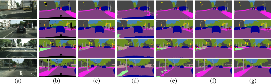
We validate the effectiveness of our proposed method by transferring our model from a synthetic dataset (GTA5 gta5 or SYNTHIA synthia) to a real-world image dataset Cityscapes Cityscapes. The Cityscapes dataset contains 2975 images for training and 500 images for validation with 19-class fine-grained semantic annotations. following outputspace, we first trained our model on the GTA5 dataset containing 19466 images and Cityscapes training set images and tested on the Cityscapes validation set for the whole 19 classes. The result is shown in Table 1. First, notice that the current state-of-the-art unsupervised model achieves 48.5 in mIoU bidir. Our model can beat it by adding 50 Cityscapes images into the training process. This proves our argument that the model can have significant improvement by adding a few target domain information. Second, the contribution of module disappears or is negative when the labeled Cityscapes images reach a number of 1000 or more compared to the oracle models. This is because the model with weak adaptation supervision overfits to the source domain so that it does not help much by adding relatively few more target images for the training process. However, the models and both have on-par improvements if trained with over 50 Cityscapes labeled images. We argue that this is due to the strong adaptation supervision. Shown in Table 2, we observe that the and structures are not very sensitive to the hyperparameters. We also provide some visualization results in Figure 3. Because is more laconic than , we only compare the model with the other baseline models on transferring from Synthia dataset containing 9400 images to Cityscapes dataset. We compare the mIoU of 13 classes shared between SYNTHIA and Cityscapes outputspace as shown in Table 3. The results can further support our arguments above.
6 Conclusion
This paper proposes a semi-supervised learning framework to adapt the global feature and the semantic-level feature from the source domain to the target domain for the semantic segmentation task. As a result, with a few labeled target images, our model outperforms current state-of-the-art unsupervised models by a great margin. Our model can also beat the oracle model trained on the whole dataset from target domain by utilizing the synthetic data with the whole target domain labeled images without suffering from the prevalent problem of overfitting to the source domain.
Acknowledgment
This work is supported by IBM-UIUC Center for Cognitive Computing Systems Research(C3SR).
References
- (1) Aleksandar Botev, Guy Lever, and David Barber. Nesterov’s accelerated gradient and momentum as approximations to regularised update descent. In IEEE IJCNN, pages 1899–1903, 2017.
- (2) Liang-Chieh Chen, George Papandreou, Iasonas Kokkinos, Kevin Murphy, and Alan L Yuille. Semantic image segmentation with deep convolutional nets and fully connected crfs. arXiv preprint arXiv:1412.7062, 2014.
- (3) Liang-Chieh Chen, George Papandreou, Iasonas Kokkinos, Kevin Murphy, and Alan L Yuille. Deeplab: Semantic image segmentation with deep convolutional nets, atrous convolution, and fully connected crfs. IEEE TPAMI, 40(4):834–848, 2017.
- (4) Liang-Chieh Chen, George Papandreou, Florian Schroff, and Hartwig Adam. Rethinking atrous convolution for semantic image segmentation. arXiv preprint arXiv:1706.05587, 2017.
- (5) Yuhua Chen, Wen Li, and Luc Van Gool. Road: Reality oriented adaptation for semantic segmentation of urban scenes. In IEEE CVPR, 2018.
- (6) Bowen Cheng, Liang-Chieh Chen, Yunchao Wei, Yukun Zhu, Zilong Huang, Jinjun Xiong, Thomas S Huang, Wen-Mei Hwu, and Honghui Shi. Spgnet: Semantic prediction guidance for scene parsing. In Proceedings of the IEEE International Conference on Computer Vision, pages 5218–5228, 2019.
- (7) Marius Cordts, Mohamed Omran, Sebastian Ramos, Timo Rehfeld, Markus Enzweiler, Rodrigo Benenson, Uwe Franke, Stefan Roth, and Bernt Schiele. The cityscapes dataset for semantic urban scene understanding. In IEEE CVPR, 2016.
- (8) Mark Everingham, S. M. Ali Eslami, Luc Van Gool, Christopher K. I. Williams, John Winn, and Andrew Zisserman. The pascal visual object classes challenge: A retrospective. IJCV, 111(1):98–136, 2015.
- (9) Yaroslav Ganin, Evgeniya Ustinova, Hana Ajakan, Pascal Germain, Hugo Larochelle, François Laviolette, Mario Marchand, and Victor Lempitsky. Domain-adversarial training of neural networks. JMLR, 17(1):2096–2030, 2016.
- (10) Ian J. Goodfellow, Jean Pouget-Abadie, Mehdi Mirza, Bing Xu, David Warde-Farley, Sherjil Ozair, Aaron Courville, and Yoshua Bengio. Generative Adversarial Networks. NIPS, 2014.
- (11) Weixiang Hong, Zhenzhen Wang, Ming Yang, and Junsong Yuan. Conditional generative adversarial network for structured domain adaptation. In IEEE CVPR, 2018.
- (12) Qibin Hou, PengTao Jiang, Yunchao Wei, and Ming-Ming Cheng. Self-erasing network for integral object attention. In NIPS, 2018.
- (13) Zilong Huang, Xinggang Wang, Jiasi Wang, Wenyu Liu, and Jingdong Wang. Weakly-supervised semantic segmentation network with deep seeded region growing. In IEEE CVPR, 2018.
- (14) Zilong Huang, Yunchao Wei, Xinggang Wang, Honghui Shi, Wenyu Liu, and Thomas S Huang. Alignseg: Feature-aligned segmentation networks. arXiv preprint arXiv:2003.00872, 2020.
- (15) Jianbo Jiao, Yunchao Wei, Zequn Jie, Honghui Shi, Rynson WH Lau, and Thomas S Huang. Geometry-aware distillation for indoor semantic segmentation. In Proceedings of the IEEE Conference on Computer Vision and Pattern Recognition, pages 2869–2878, 2019.
- (16) Diederik P. Kingma and Jimmy Ba. Adam: A Method for Stochastic Optimization. In ICLR, 2014.
- (17) Andrew L. Maas, Awni Y Hannun, and Andrew Ng. Rectifier nonlinearities improve neural network acoustic models. In ICML, 2013.
- (18) Yunsheng Li, Lu Yuan, and Nuno Vasconcelos. Bidirectional learning for domain adaptation of semantic segmentation. In The IEEE Conference on Computer Vision and Pattern Recognition (CVPR), June 2019.
- (19) Rui Qian, Yunchao Wei, Honghui Shi, Jiachen Li, Jiaying Liu, and Thomas Huang. Weakly supervised scene parsing with point-based distance metric learning. In Proceedings of the AAAI Conference on Artificial Intelligence, volume 33, pages 8843–8850, 2019.
- (20) Stephan R. Richter, Vibhav Vineet, Stefan Roth, and Vladlen Koltun. Playing for data: Ground truth from computer games. In ECCV, 2016.
- (21) German Ros, Laura Sellart, Joanna Materzynska, David Vazquez, and Antonio Lopez. The SYNTHIA Dataset: A large collection of synthetic images for semantic segmentation of urban scenes. In IEEE CVPR, 2016.
- (22) Fatemeh Saleh, Sadegh Aliakbarian, Mathieu Salzmann, Lars Petersson, and Jose M. Alvarez. Effective use of synthetic data for urban scene semantic segmentation. In ECCV, 2018.
- (23) Swami Sankaranarayanan, Yogesh Balaji, Arpit Jain, Ser-Nam Lim, and Rama Chellappa. Unsupervised domain adaptation for semantic segmentation with gans. In IEEE CVPR, 2018.
- (24) Yi-Hsuan Tsai, Wei-Chih Hung, Samuel Schulter, Kihyuk Sohn, Ming-Hsuan Yang, and Manmohan Chandraker. Learning to adapt structured output space for semantic segmentation. In IEEE CVPR, 2018.
- (25) Mei Wang and Weihong Deng. Deep visual domain adaptation: A survey. Neurocomputing, 312:135–153, 2018.
- (26) Zhonghao Wang, Mo Yu, Yunchao Wei, Rogerior Feris, Jinjun Xiong, Wen mei Hwu, Thomas S. Huang, and Honghui Shi. Differential treatment for stuff and things: A simple unsupervised domain adaptation method for semantic segmentation. arXiv preprint arXiv:2003.08040, 2020.
- (27) Yunchao Wei, Jiashi Feng, Xiaodan Liang, Ming-Ming Cheng, Yao Zhao, and Shuicheng Yan. Object region mining with adversarial erasing: A simple classification to semantic segmentation approach. In IEEE CVPR, 2017.
- (28) Yunchao Wei, Xiaodan Liang, Yunpeng Chen, Xiaohui Shen, Ming-Ming Cheng, Jiashi Feng, Yao Zhao, and Shuicheng Yan. Stc: A simple to complex framework for weakly-supervised semantic segmentation. IEEE TPAMI, 39(11):2314–2320, 2017.
- (29) Yunchao Wei, Huaxin Xiao, Honghui Shi, Zequn Jie, Jiashi Feng, and Thomas S. Huang. Revisiting dilated convolution: A simple approach for weakly- and semi-supervised semantic segmentation. In IEEE CVPR, 2018.
- (30) Zuxuan Wu, Xintong Han, Yen-Liang Lin, Mustafa Gökhan Uzunbas, Tom Goldstein, Ser-Nam Lim, and Larry S. Davis. DCAN: dual channel-wise alignment networks for unsupervised scene adaptation. In ECCV, 2018.
- (31) Yiheng Zhang, Zhaofan Qiu, Ting Yao, Dong Liu, and Tao Mei. Fully convolutional adaptation networks for semantic segmentation. In IEEE CVPR, 2018.
- (32) Hengshuang Zhao, Jianping Shi, Xiaojuan Qi, Xiaogang Wang, and Jiaya Jia. Pyramid scene parsing network. In IEEE CVPR, 2017.
Appendix A State-of-the-art comparison
| GTA5 Cityscapes | ||||||||||||||||||||
| Method |
road |
sidewalk |
building |
wall |
fence |
pole |
light |
sign |
vegetation |
terrain |
sky |
person |
rider |
car |
truck |
bus |
train |
motorbike |
bike |
mIoU |
| Wu et al.wu | 85.0 | 30.8 | 81.3 | 25.8 | 21.2 | 22.2 | 25.4 | 26.6 | 83.4 | 36.7 | 76.2 | 58.9 | 24.9 | 80.7 | 29.5 | 42.9 | 2.5 | 26.9 | 11.6 | 41.7 |
| Tsai et al.outputspace | 86.5 | 36.0 | 79.9 | 23.4 | 23.3 | 23.9 | 35.2 | 14.8 | 83.4 | 33.3 | 75.6 | 58.5 | 27.6 | 73.7 | 32.5 | 35.4 | 3.9 | 30.1 | 28.1 | 42.4 |
| Saleh et al.saleh | 79.8 | 29.3 | 77.8 | 24.2 | 21.6 | 6.9 | 23.5 | 44.2 | 80.5 | 38.0 | 76.2 | 52.7 | 22.2 | 83.0 | 32.3 | 41.3 | 27.0 | 19.3 | 27.7 | 42.5 |
| Hong et al.hong | 89.2 | 49.0 | 70.7 | 13.5 | 10.9 | 38.5 | 29.4 | 33.7 | 77.9 | 37.6 | 65.8 | 75.1 | 32.4 | 77.8 | 39.2 | 45.2 | 0.0 | 25.5 | 35.4 | 44.5 |
| oracle wholecity | 96.7 | 75.7 | 88.3 | 46.0 | 41.7 | 42.6 | 47.9 | 62.7 | 88.8 | 53.5 | 90.6 | 69.1 | 49.7 | 91.6 | 71.0 | 73.6 | 45.3 | 52.0 | 65.5 | 65.9 |
| ours+50city | 94.3 | 63.0 | 84.5 | 26.8 | 28.0 | 38.4 | 35.5 | 48.7 | 87.1 | 39.2 | 88.8 | 62.2 | 16.3 | 87.6 | 23.2 | 39.2 | 7.2 | 24.4 | 58.1 | 50.1 |
| ours+100city | 96.0 | 71.7 | 85.9 | 27.9 | 27.6 | 42.8 | 44.7 | 55.9 | 87.7 | 46.9 | 89.0 | 66.0 | 36.4 | 88.4 | 28.9 | 21.4 | 11.4 | 38.0 | 63.2 | 54.2 |
| ours+200city | 96.1 | 71.9 | 85.8 | 28.4 | 29.8 | 42.5 | 45.0 | 56.2 | 87.4 | 45.0 | 88.7 | 65.8 | 38.2 | 89.6 | 42.2 | 35.9 | 17.1 | 35.8 | 61.6 | 56.0 |
| ours+500city | 96.2 | 72.7 | 87.6 | 35.1 | 31.7 | 46.6 | 46.9 | 62.7 | 88.7 | 49.6 | 90.5 | 69.2 | 42.7 | 91.1 | 52.6 | 60.9 | 9.6 | 43.1 | 65.6 | 60.2 |
| ours+1000city | 96.8 | 76.3 | 88.5 | 30.5 | 41.7 | 46.5 | 51.3 | 64.3 | 89.1 | 54.2 | 91.0 | 70.7 | 48.7 | 91.6 | 59.9 | 68.0 | 40.8 | 48.0 | 67.0 | 64.5 |
| ours+2975city(all) | 97.3 | 79.3 | 89.8 | 47.4 | 49.7 | 48.9 | 52.9 | 67.4 | 89.7 | 56.3 | 91.9 | 72.2 | 53.1 | 92.6 | 69.3 | 78.4 | 58.0 | 51.2 | 68.2 | 69.1 |
| SYNTHIA Cityscapes | ||||||||||||||
| Method |
road |
sidewalk |
building |
light |
sign |
vegetation |
sky |
person |
rider |
car |
bus |
motorbike |
bike |
mIoU |
| Wu et al.wu | 81.5 | 33.4 | 72.4 | 8.6 | 10.5 | 71.0 | 68.7 | 51.5 | 18.7 | 75.3 | 22.7 | 12.8 | 28.1 | 42.7 |
| Tsai et al.outputspace | 84.3 | 42.7 | 77.5 | 4.7 | 7.0 | 77.9 | 82.5 | 54.3 | 21.0 | 72.3 | 32.2 | 18.9 | 32.3 | 46.7 |
| Hong et al.hong | 85.0 | 25.8 | 73.5 | 19.5 | 21.3 | 67.4 | 69.4 | 68.5 | 25.0 | 76.5 | 41.6 | 17.9 | 29.5 | 47.8 |
| oracle wholecity | 96.5 | 77.6 | 91.2 | 49.0 | 62.1 | 91.4 | 90.2 | 70.1 | 47.7 | 91.8 | 74.9 | 50.1 | 66.9 | 73.8 |
| ours+50city | 94.1 | 63.9 | 87.6 | 18.1 | 37.1 | 87.5 | 89.7 | 64.6 | 37.0 | 87.4 | 38.6 | 23.2 | 59.6 | 60.7 |
| ours+100city | 93.6 | 64.6 | 88.8 | 30.4 | 43.3 | 89.0 | 89.2 | 65.3 | 25.1 | 88.2 | 47.4 | 23.8 | 59.2 | 62.1 |
| ours+200city | 95.2 | 71.2 | 89.1 | 32.9 | 46.4 | 89.1 | 90.3 | 67.0 | 31.6 | 89.4 | 42.3 | 32.9 | 64.8 | 64.8 |
| ours+500city | 96.7 | 77.1 | 91.0 | 42.6 | 62.2 | 91.2 | 91.3 | 69.5 | 34.8 | 91.6 | 56.3 | 35.0 | 68.0 | 69.8 |
| ours+1000city | 97.2 | 80.6 | 91.3 | 46.3 | 66.4 | 91.5 | 91.4 | 71.6 | 45.0 | 92.2 | 61.5 | 45.3 | 68.4 | 73.0 |
| ours+2975city(all) | 97.5 | 82.7 | 92.4 | 53.3 | 69.7 | 92.2 | 92.8 | 73.6 | 52.4 | 93.7 | 79.3 | 50.9 | 71.5 | 77.1 |