Radiative decay of $\Xi_{b}(6227)$ in a hadronic molecule picture

In the past five years, many new narrow bottom baryons were discovered. The latest one is in 2018, the LHCb Collaboration observed a new narrow structure with the statistical significance of 9.2 $\sigma$ in the $\Lambda_{b}^{0}K^{-}$ and $\Xi_{b}^{0}\pi^{-}$ invariant mass spectra, named $\Xi_{b}(6227)^{-}$ Aaij:2018yqz. The observed resonance parameters of the structure are

respectively. The observed channel indicates the isospin of the $\Xi_{b}(6227)^{-}$ is $1/2$.

However, its spin-parity has not been determined in the experiment. Assuming different assignments for its spin-parity, some theoretical interpretations were already discussed in the literature. Considering $\Xi_{b}(6227)$ as a conventional bottom baryon, the spin-parity was assigned to be $J^{P}=3/2^{-}$ or $J^{P}=5/2^{-}$ in Refs. Chen:2018orb; Wang:2018fjm; Aliev:2018lcs; Chua:2018lfa; Cui:2019dzj. Besides supposing $\Xi_{b}(6227)$ to be a conventional bottom baryon, the $\Xi_{b}(6227)$ was explained as a $S-$ wave dynamically generated resonance with a dominant $\bar{K}\Sigma_{b}$ configuration Yu:2018yxl; Nieves:2019jhp. However, a different conclusion was got that the $\Xi_{b}(6227)$ can be identified as a pure $\bar{K}\Sigma_{b}$ bound state with $J^{P}=1/2^{-}$ Huang:2018bed.

To date, the inner structure of this state remains unclear, and more efforts are necessary. On the theoretical side, the study on the decay properties may provide a way of learning about the nature of the $\Xi_{b}(6227)$. Regarding the $\Xi_{b}(6227)$ as a conventional bottom baryon, the strong decay width has been computed Chen:2018orb; Wang:2018fjm; Aliev:2018lcs; Chua:2018lfa; Cui:2019dzj. The results indicate that the $\Xi_{b}(6227)$ can be well interpreted as a conventional three quark state in comparison with the experimental total width. However, the $S-$ wave $\bar{K}\Sigma_{b}$ assignment for the $\Xi_{b}(6227)$ is also supported by studying the strong decay widths Yu:2018yxl; Nieves:2019jhp; Huang:2018bed. One finds that the two-body allowed strong decay widths from different model are consistent with each other within errors. In other word, based on the analysis of the two-body allowed strong decays, the $\Xi_{b}(6227)$ is not only can be considered as a conventional three quark state, but also can be considered as a $S$-wave $\bar{K}\Sigma_{b}$ molecular. Theoretical investigations on other decay modes will be very helpful to determine whether the $\Xi_{b}(6227)$ is a conventional bottom baryon or a molecular state.

The radiative decays may be helpful to distinguish the internal structure of the $\Xi_{b}(6227)$, since the coupling of the photon to the constituent $\bar{K}$ meson and $\Sigma_{b}$ baryon of the $\Xi_{b}(6227)$ is essentially different from that of the quark models for which the photon directly couples to the quark system Koniuk:1979vy. Therefore, a precise measurements of the radiative decays can be quite useful to test the different interpretations of the $\Xi_{b}(6227)$. However, no work has been done to discuss the radiation decays of the $\Xi(6227)$. In the present work we continue our study of the $\Xi_{b}(6227)$ properties considering its radiative decays in the hadronic molecule approach developed in our previously paper Huang:2018bed.

This work is organized as follows. The theoretical formalism is explained in Sec. II. The predicted partial decay widths are presented in Sec. III, followed by a short summary in the last section.

In our previous paper Huang:2018bed, the $\Xi_{b}(6227)$ is interpreted as a pure $\bar{K}\Sigma_{b}$ bound state with $J^{P}=1/2^{-}$ by studying the strong decay model, where consistency with the observed strong decay width of the $\Xi_{b}(6227)$ was achieved in a hadronic molecule interpretation Huang:2018bed. According to the pure $\bar{K}\Sigma_{b}$ molecular scenario, we calculate the radiative decay widths $\Xi_{b}(6227)\to\Xi_{b}\gamma$ and $\Xi_{b}(6227)\to\Xi_{b}^{{}^{\prime}}\gamma$ in this work, that would help to understand the internal structure of the $\Xi_{b}(6227)$. In the $\bar{K}\Sigma_{b}$ molecular scenario, the $\Xi_{b}(6227)$ should couple to its components via $S-$ wave, and the corresponding effective Lagrangian is in the form Huang:2018bed; Dong:2010gu

where $\omega_{ij}=m_{i}/(m_{i}+m_{j})$ with $m_{i}$ is the mass of the baryon or meson. $k_{1}$ and $k_{2}$ is four-momenta of the $\bar{K}$ meson and $\Sigma_{b}$ baryon, respectively. From Refs. Huang:2018bed; Dong:2010gu; Faessler:2007gv; Dong:2010xv, we find that the correlation function $\Phi(p^{2})\doteq\exp(-p_{E}^{2}/\Lambda^{2})$ is not only introduced to describe the distributions of the $\bar{K}$ meson and $\Sigma_{b}$ baryon in the hadronic molecule but also plays a role to stop the Feynman diagrams ultraviolet divergence. The $p_{E}$ being the Euclidean Jacobi momentum and the $\Lambda$ being the size parameter which characterizes the distribution of the components inside the molecule. It should be noted that the $\Lambda$ is a free parameter and it is usually chosen to be about $1$ GeV to reproduce the experimental observed decay width in the literature Huang:2018bed; Dong:2010gu; Faessler:2007gv; Dong:2010xv. In this work, we vary $\Lambda$ in a range of 0.9 GeV $\leq\Lambda\leq{}1.10$ GeV.

In the above Lagrangian, the remaining unknown coupling constant $g_{\Xi_{b}(6227)\Sigma_{b}\bar{K}}$ can be computed by the compositeness condition Weinberg:1962hj; Salam:1962ap, which indicates that the renormalization constants of a composite particle wave function should be zero, i.e.,

where the ${\cal{S}}[\Xi_{b}(6227)]$ is the mass operator of the $\Xi_{b}(6227)$ corresponding to the diagrams in Fig. 1. With the effective Lagrangian in Eq. (2) and the compositeness condition in Eq. (3), we can obtain the coupling constant of the $\Sigma_{b}\bar{K}$ molecule to its components

where ${\cal{F}}_{i}=-2\omega_{i}^{2}+\frac{\Delta^{2}_{i}}{4z}-\beta$ and $\Delta_{i}=-4\omega_{i}-2\beta$ with $i=1$ and $2$ denoting the molecule component $K^{-}\Sigma_{b}^{0}$ and $\bar{K}^{0}\Sigma_{b}^{-}$, respectively. ${\cal{M}}_{i}$ and $m_{i}$ are the mass of the $\Sigma_{b}$ baryon and the mass of the $\bar{K}$ meson, respectively. The isospin-spin symmetry requires the coupling of the $\Xi_{b}^{-}\Sigma_{b}^{-}\bar{K}^{0}$ vertex is $\sqrt{2}$ times lager than the one of the $\Xi_{b}^{-}\Sigma_{b}^{0}K^{-}$. Simply employing those ratios and the ${\cal{A}}_{i}$ listed

In the present hadronic molecular scenario, the diagrams contributing to the $\Xi_{b}(6227)^{-}\to\Xi^{-}_{b}\gamma$ and $\Xi_{b}(6227)^{-}\to\Xi_{b}^{{}^{\prime}-}\gamma$ decay are presented in Fig. 2.

In order to compute the radiative decays of the diagrams shown in Fig. 2, the effective Lagrangian densities related to the photon fields are needed, which are Chen:2010re; Kim:2014hha

where the strength tensor are defined as $F_{\mu\nu}=\partial_{\mu}A_{\nu}-\partial_{\nu}A_{\mu}$ and $K^{*}_{\mu\nu}=\partial_{\mu}K^{*}_{\nu}-\partial_{\nu}K^{*}_{\mu}$. The $\alpha=e^{2}/4\pi=1/137$ is the electromagnetic fine structure constant. The $\mu_{\Sigma_{b}\Lambda_{b}}=-1.37{}\mu$ is transition magnetic moment Wang:2018cre, which $\mu$ is in the unit of the nuclear magneton. The coupling constant $g_{K^{*+}K^{+}\gamma}$ and $g_{K^{*0}K^{0}\gamma}$ can be determined from the partial decay width of $K^{*+}\to{}K^{+}\gamma$ and $K^{*0}\to{}K^{0}\gamma$, which can be obtained from Eq. (6),

where $m_{K^{*}}$ and $m_{K}$ are mass of $K^{*}$ and kaon, respectively.

According to the experimental widths $\Gamma(K^{*+}\to{}K^{+}\gamma)=0.0503$ KeV Tanabashi:2018oca, $\Gamma(K^{*0}\to{}K^{0}\gamma)=0.125$ KeV Tanabashi:2018oca, and the masses of the particles that shown in Table 1, the coupling constant $g_{K^{*}K\gamma}$ is fixed as

The signs of these coupling constants are fixed by the quark model.

To evaluate the diagrams in Fig. 2, in addition to the Lagrangian in Eqs.( 2, 6, 7), the following effective Lagrangians, responsible for heavy baryons and pseudoscalar mesons interactions are needed as well Meng:2018gan

Where the coupling constant $g_{1}=-\sqrt{\frac{8}{3}}g_{2}$ and $g_{6}=0$ Meng:2018gan. $u^{\mu}$ is the axial vector combination of the pseudoscalar-meson fields and its derivatives,

where the $u^{2}=U=\exp(i\frac{\phi}{f_{0}})$, $f_{0}$=92.4 MeV, and the pseudoscalar-meson octet $\phi$ are represented by the $3\times 3$ matrix

The particle assignment for the $J=1/2$ bottom baryons of the $B_{\bar{3}}$ and $B_{6}$ representations is Meng:2018gan; Banuls:1999br

The coupling $g_{2}$ is fixed from the strong decay width of $\Sigma_{b}\to{}\Lambda_{b}^{0}\pi$. With the help of Eqs. (12-16), the two-body decay width $\Gamma(\Sigma_{b}\to{}\Lambda_{b}^{0}\pi)$ is related to $g_{2}$ as

where the $m_{\Sigma_{b}}$, $m_{\Lambda_{b}^{0}}$, and $m_{\pi}$ are the masses of the $\Sigma_{b}$ baryon, $\Lambda_{b}^{0}$ baryon, and $\pi$ meson, respectively. The ${\cal{P}}_{\pi{}\Lambda_{b}^{0}}$ is the three-momentum of the $\pi$ in the rest frame of the $\Sigma_{b}$. Particle Data Group list the $\Sigma_{b}$ predominantly decays into $\Lambda_{b}^{0}\pi$ Tanabashi:2018oca, so its partial width may be approximately equal to the total width of the $\Sigma_{b}$. Using the experimental strong decay width and the masses of the particles needed in the present work we obtain $g_{2}=0.252\pm{}0.013$.

To compute the radiative decay amplitude, the $K^{*-}\Sigma^{0}_{b}\Xi_{b}^{-(^{\prime})}$ and $\bar{K}^{*0}\Sigma^{-}_{b}\Xi_{b}^{-(^{\prime})}$ vertices Lagrangian are also needed. Following the strategy of Ref. Hofmann:2005sw; Montana:2017kjw, the Lagrangian for the $K^{*-}\Sigma^{0}_{b}\Xi_{b}^{-(^{\prime})}$ and $\bar{K}^{*0}\Sigma^{-}_{b}\Xi_{b}^{-(^{\prime})}$ vertexes can be easily obtained by replacing the charm baryons with the bottom ones, whose procedures are just illustrated in Ref. Huang:2018bed,

where the coupling constant $g=6.6$ and is get from Ref. Montana:2017kjw.

In the radiative decay of the $\Xi_{b}(6227)^{-}\to\Xi_{b}^{-}\gamma$ and $\Xi_{b}(6227)^{-}\to\Xi_{b}^{{}^{\prime}-}\gamma$, the photon can be emitted from the kaon meson and $\Sigma_{b}$ baryon. The triangle diagrams are listed in Fig. 2 and the corresponding amplitudes are

The total amplitude of $\Xi_{b}(6227)^{-}\to\Xi_{b}^{-(^{\prime})}\gamma$ is

After performing the loop integral, the total contributions of the triangle diagrams to the $\Xi_{b}(6227)^{-}\to\Xi_{b}^{-(^{\prime})}\gamma$ can be parameterized as

One should notice that this amplitude can not satisfies the gauge invariance of the photon field if only triangle diagrams are included. To ensure the gauge invariance of the total amplitudes, the contact diagram in Fig. 3 should be included. The effective Lagrangian describing vertex of $\Xi_{b}^{(^{\prime})}\gamma\Sigma_{b}\bar{K}$ could be deduced from the one of the $\Xi_{b}^{(^{\prime})}\Sigma_{b}\bar{K}$ by minimal substitution $\partial^{\mu}\to\partial^{\mu}+ie{\cal{A}}^{\mu}$, which is

By this effective Lagrangian, the amplitude of the contact diagram is in the form,

After performing the loop integral in the above amplitude, we get,

The total amplitude of the $\Xi_{b}(6227)^{-}\to\Xi_{b}^{-(^{\prime})}\gamma$ is the sum of the triangle diagrams contributions and the contact term contributions. In order to keep the full amplitude gauge invariant, the $g_{Con}=-g_{1}^{Tri}-g_{2}^{Tri}$ can be got and the coupling constant $g_{1}^{Tri}$ and $g_{2}^{Tri}$ could be evaluated from the amplitudes listed in Eqs. 19.

Once the amplitudes are determined, the corresponding partial decay widths can be obtained, which read,

where $J$ is the total angular momentum of the $\Xi_{b}(6227)$ state, the $|\vec{p}_{1}|$ is the three-momenta of the decay products in the center of mass frame, the overline indicates the sum over the polarization vectors of the final hadrons, and $MB$ denotes the decay channel of $MB$, i.e.,$\Xi_{b}\gamma$ and $\Xi_{b}^{{}^{\prime}}\gamma$.

To estimate the radiative decay widths of the considered processes, the relevant coupling constants $g_{\Xi_{b}(6227)\Sigma_{b}\bar{K}}$ should be first discussed. Regarding the $\Xi_{b}(6227)$ as $S-$wave loosely $\Sigma_{b}\bar{K}$ hadronic molecule, the coupling constant $g_{\Xi_{b}(6227)\Sigma_{b}\bar{K}}$ can be computed via compositeness condition. As shown in Eq. 4, the coupling constant is dependent on the parameter $\Lambda$. With a value of the cutoff $\Lambda=0.9-1.1$ GeV, the corresponding coupling constant is varying from 2.68 GeV to 2.47 GeV, which is shown in Fig. 4. We note that the coupling constant decreases slowly with the increase of the cut-off, and the coupling constant is almost independent of $\Lambda$. In our previous paper Huang:2018bed, the coupling constant is incorrect and is smaller than that given in this paper. However, it does not change the conclusion that $\Xi_{b}(6227)$ only can be considered as $S-$wave $\bar{K}\Sigma_{b}$ molecule and the new result is shown in Fig. 4.

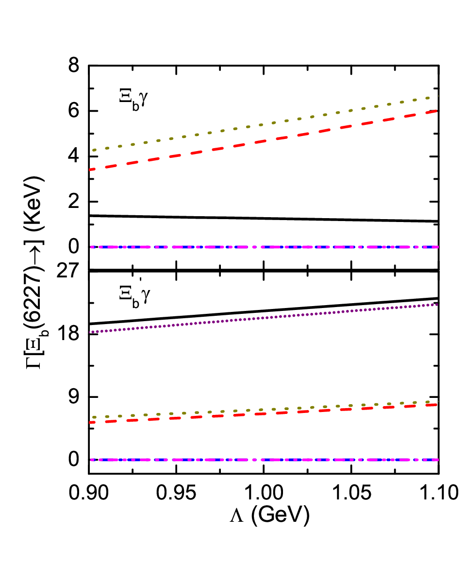
In Fig. 5, the dependence of the radiative decay widths on the cutoff $\Lambda$ is shown. With the increasing of cut-off from 0.9 GeV to 1.1 GeV, the radiative decay width of the $\Xi_{b}(6227)\to\gamma\Xi^{{}^{\prime}}_{b}$ monotonously increases, but very slowly. In particular, the partial width varies from 19.47 to 23.15 KeV with the variation of $\Lambda$ from 0.9 to 1.1 GeV. However, the radiative decay widths decreases for the $\Xi_{b}(6227)\to\gamma\Xi_{b}$ when we change the cut-off $\Lambda$ from 0.9 to 1.1 GeV. With the constrained parameter $\Lambda$, the partial width of the $\Xi_{b}(6227)\to\gamma\Xi_{b}$ is estimated to be

which is very weakly dependent on the model parameter. Our calculation indicates that the width of $\Xi_{b}(6227)\to\gamma\Xi^{{}^{\prime}}_{b}$ is about one order larger than the one of $\Xi_{b}(6227)\to\gamma\Xi_{b}$.

The contribution to the total width coming from individual channels are also shown in Fig. 5. Since the relative signs of the corresponding amplitude in Fig. 2 are well defined, this makes us easy to analyze the character of the interferences between the various channels. The total decay widths obtained are the square of their coherent sum. As for the $\Xi_{b}(6227)\to\gamma\Xi_{b}$ process, the $K^{-}$-exchange and contract term provide a dominant contributions to the total decay width, and the amplitude of these two channels are not gauge invariant. The amplitudes corresponding to $\Lambda_{b}^{0}$-exchange and $\bar{K}^{*}$-exchange are gauge invariant and the number results indicate that the contribution of these amplitudes are almost three order smaller than that of the amplitudes corresponding to $K^{-}$-exchange and contract term. However, the interferences among them are sizable, which make the total radiative decay width smaller than the partial decay widths of the $K^{-}$-exchange and contact term, respectively. For the transition $\Xi_{b}(6227)\to\gamma\Xi^{{}^{\prime}}_{b}$, the individual contributions of the $\Lambda_{b}^{0}$ exchange provides a dominant over the others, which almost equal to the total width. One finds that the estimated these individual partial decay widths are all insensitive to the $\Lambda$. It should be noted that the radiative decay width of the $\Xi_{b}(6227)$ into $\gamma\Xi_{b}$ final state is about one order smaller than into $\gamma\Xi^{{}^{\prime}}_{b}$ final state due to the contribution of Fig. 2(b) vanishes in the case of $\Xi_{b}(6227)\to\gamma\Xi_{b}$.

According to the Eq. 10 and the experimental width $\Gamma(K^{*0}\to{}K^{0}\gamma)$=0.125 KeV, the coupling constant $g_{K^{*0}K^{0}\gamma}$=0.904 GeV^-1 is fixed. However, it is usual chosen as about -0.904 GeV^-1 in the literature and the sign of this coupling constant is fixed by the quark model. If we take $g_{K^{*0}K^{0}\gamma}$=0.904 GeV^-1, the decay width $\Gamma_{\gamma{}\Xi_{b}}$=1.39-1.15 KeV and $\Gamma_{\gamma{}\Xi^{{}^{\prime}}_{b}}$=19.33-23.08 KeV are very close to previous results:$\Gamma_{\gamma{}\Xi_{b}}$=1.38-1.14 KeV and $\Gamma_{\gamma{}\Xi^{{}^{\prime}}_{b}}$=19.47-23.15 KeV. In other words, our numerical results show that the value of the decay width $\Gamma_{\gamma{}\Xi_{b}}$ and $\Gamma_{\gamma{}\Xi^{{}^{\prime}}_{b}}$ are not very sensitive to the negative sign when varying the model parameter $\Lambda$ from 0.9 to 1.1 .

At present, there in no sufficient experimental information to determine the spin-parity of $\Xi_{b}(6227)$ state. The study of its decay behaviors at some experimental could provide a further test to the inner structure. However, the strong decay channels are hard to determine whether the $\Xi_{b}(6227)$ is a conventional bottom baryon Chen:2018orb; Wang:2018fjm; Aliev:2018lcs; Chua:2018lfa; Cui:2019dzj or a molecular state Yu:2018yxl; Nieves:2019jhp; Huang:2018bed.

In the present work, we estimated the partial widths for the radiative from the $\Xi_{b}(6227)$ to the $\Xi^{{}^{\prime}}_{b}$ and $\Xi_{b}$ in a molecular scenario, in which the $\Xi_{b}(6227)$ is assigned as a $\Sigma_{b}{}\bar{K}$ hadronic molecule. In the considered parameter region, the partial widths are evaluated to be

Our estimations indicated that the partial widths for the $\Xi_{b}(6227)\to\gamma\Xi_{b}$ is about one order smaller than that of $\Xi_{b}(6227)\to\gamma\Xi^{{}^{\prime}}_{b}$.

Basing on the current integrated luminosity and our estimations, the facilities like LHCb might have the capability to detect radiative decays of $\Xi_{b}(6227)$ baryon in the keV regime. Such research can also be done in the forthcoming Belle II experiment. The study of the radiative decay of $\Xi_{b}(6227)$ with quark model is strongly recommended. In comparison with the predicted widths of quark model, the results in present work can provide further information for the experimental search for the $\Xi_{b}(6227)$, and, on the other hand, the experimental measurements for these radiative decay processes could be a crucial test for the molecule interpretation of the $\Xi_{b}(6227)$.

References

• (1) R. Aaij et al. [LHCb Collaboration], Observation of a new Ξb−\Xi_{b}^{-} resonance, Phys. Rev. Lett. 121, 072002 (2018).
• (2) B. Chen, K. W. Wei, X. Liu and A. Zhang, Role of newly discovered Ξb​(6227)−\Xi_{b}(6227)^{-} for constructing excited bottom baryon family, Phys. Rev. D 98, 031502 (2018).
• (3) K. L. Wang, Q. F. L¨¹ and X. H. Zhong, Phys. Rev. D 99, 014011 (2019).
• (4) T. M. Aliev, K. Azizi, Y. Sarac and H. Sundu, Structure of the Ξb​(6227)−\Xi_{b}(6227)^{-} resonance, Phys. Rev. D 98, 094014 (2018).
• (5) C. K. Chua, Color-allowed bottom baryon to charmed baryon nonleptonic decays, Phys. Rev. D 99, 014023 (2019).
• (6) E. L. Cui, H. M. Yang, H. X. Chen and A. Hosaka, Identifying the Ξb​(6227)\Xi_{b}(6227) and Σb​(6097)\Sigma_{b}(6097) as PP-wave bottom baryons of JP=3/2−J^{P}=3/2^{-}, Phys. Rev. D 99, 094021 (2019).
• (7) Q. X. Yu, R. Pavao, V. R. Debastiani and E. Oset, Description of the Ξc\Xi_{c} and Ξb\Xi_{b} states as molecular states, Eur. Phys. J. C 79, 167 (2019).
• (8) J. Nieves, R. Pavao and L. Tolos, Ξc\Xi_{c} and Ξb\Xi_{b} excited states within a SU(6)lsf×{\rm SU(6)}_{\rm lsf}\timesHQSS model, arXiv:1911.06089 [hep-ph].
• (9) Y. Huang, C. j. Xiao, L. S. Geng and J. He, Strong decays of the Ξb​(6227)\Xi_{b}(6227) as a Σb​K¯\Sigma_{b}\bar{K} molecule, Phys. Rev. D 99, 014008 (2019).
• (10) R. Koniuk and N. Isgur, Baryon Decays in a Quark Model with Chromodynamics, Phys. Rev. D 21, 1868 (1980) Erratum: [Phys. Rev. D 23, 818 (1981)].
• (11) Y. Dong, A. Faessler, T. Gutsche and V. E. Lyubovitskij, Charmed baryon Sigmac(2800) as a ND hadronic molecule, Phys. Rev. D 81, 074011 (2010).
• (12) A. Faessler, T. Gutsche, V. E. Lyubovitskij and Y. L. Ma, Strong and radiative decays of the Ds​0∗​(2317)D_{s0}^{*}(2317) meson in the DK-molecule picture, Phys. Rev. D 76, 014005 (2007).
• (13) Y. Dong, A. Faessler, T. Gutsche, S. Kumano and V. E. Lyubovitskij, Radiative decay of Λc​(2940)+\Lambda_{c}(2940)^{+} in a hadronic molecule picture, Phys. Rev. D 82, 034035 (2010).
• (14) S. Weinberg, Elementary particle theory of composite particles, Phys. Rev. 130, 776 (1963).
• (15) A. Salam, Lagrangian theory of composite particles, Nuovo Cim. 25, 224 (1962).
• (16) D. Y. Chen, Y. B. Dong and X. Liu, Long-distant contribution and χc​1\chi_{c1} radiative decays to light vector meson, Eur. Phys. J. C 70, 177 (2010).
• (17) S. H. Kim, A. Hosaka and H. C. Kim, Effects of N⁡(2000)​ 5/2+N(2000)\,5/2^{+}, N⁡(2060)​ 5/2−N(2060)\,5/2^{-}, N⁡(2120)​ 3/2−N(2120)\,3/2^{-}, and N⁡(2190)​ 7/2−N(2190)\,7/2^{-} on K∗​ΛK^{*}\Lambda photoproduction, Phys. Rev. D 90, 014021 (2014).
• (18) G. J. Wang, L. Meng and S. L. Zhu, Radiative decays of the singly heavy baryons in chiral perturbation theory, Phys. Rev. D 99, 034021 (2019).
• (19) M. Tanabashi et al. [Particle Data Group], Review of Particle Physics, Phys. Rev. D 98, 030001 (2018).
• (20) L. Meng, G. J. Wang, C. Z. Leng, Z. W. Liu and S. L. Zhu, Magnetic moments of the spin-32{3\over 2} singly heavy baryons, Phys. Rev. D 98, 094013 (2018).
• (21) M. C. Banuls, A. Pich and I. Scimemi, Electromagnetic decays of heavy baryons, Phys. Rev. D 61, 094009 (2000).
• (22) J. Hofmann and M. F. M. Lutz, Coupled-channel study of crypto-exotic baryons with charm, Nucl. Phys. A 763, 90 (2005).
• (23) G. Montan~\tilde{n}a, A. Feijoo and ¨¤. Ramos, A meson-baryon molecular interpretation for some Ωc\Omega_{c} excited states, Eur. Phys. J. A 54, 64 (2018).