Diagrammatic Monte Carlo Method for Impurity Models with General Interactions and Hybridizations
Abstract
We present a diagrammatic Monte Carlo method for quantum impurity problems with general interactions and general hybridization functions. Our method uses a recursive determinant scheme to sample diagrams for the scattering amplitude. Unlike in other methods for general impurity problems, an approximation of the continuous hybridization function by a finite number of bath states is not needed, and accessing low temperature does not incur an exponential cost. We test the method for the example of molecular systems, where we systematically vary temperature, interatomic distance, and basis set size. We further apply the method to an impurity problem generated by a self-energy embedding calculation of correlated antiferromagnetic NiO. We find that the method is ideal for quantum impurity problems with a large number of orbitals but only moderate correlations.
I Introduction
Quantum impurity models, originally introduced to describe magnetic impurities such as iron or copper atoms with partially filled d-shells in a non-magnetic host material Anderson 1961, have since found applications in nanoscience as representations of quantum dots and molecular conductors Hanson et al. 2007, and in surface science to understand the adsorption of atoms on surfaces Brako and Newns 1981; Langreth and Nordlander 1991. In addition, they form the central part of embedding theories such as the dynamical mean field theory (DMFT) Georges et al. 1996; Kotliar et al. 2006 and its variants Lichtenstein and Katsnelson 2000; Kotliar et al. 2001; Hettler et al. 2000; Maier et al. 2005; Anisimov et al. 1997; Lichtenstein and Katsnelson 1998; Held et al. 2006; Sun and Kotliar 2002; Biermann et al. 2003; Biermann et al. 2005; Boehnke et al. 2016; Choi et al. 2016; Lee and Haule 2017, as well as the self-energy embedding theory (SEET) Kananenka et al. 2015; Lan et al. 2015; Lan et al. 2016, where they describe the behavior of a few ‘strongly correlated’ orbitals embedded into a weakly correlated or non-interacting background of other orbitals. These methods promise a systematic route for the simulation of strongly correlated quantum many-body problems Zgid and Gull 2017.
While the original formulation of a quantum impurity model Anderson 1961 only describes a single correlated orbital coupled to a non-interacting environment, in general the impurities occurring in the context of surface science and embedding theories contain many orbitals with general four-fermion interactions and few symmetries Mazurenko et al. 2010. The time-dependent hybridization function describing the hopping between the impurity and its environment is typically such that it cannot be diagonalized for all frequencies at once.
Solving quantum impurity problems, i.e. obtaining the impurity Green’s function given an impurity Hamiltonian and a hybridization function, requires the use of numerical methods. A wide range of such methods exist. Hamiltonian-based methods, such as exact diagonalization Caffarel and Krauth 1994; Capone et al. 2004; Koch et al. 2008; Liebsch and Tong 2009; Sénéchal 2010 and its variants Lu et al. 2014, configuration-interactions Zgid et al. 2012, or coupled cluster theory Shee and Zgid 2019; Zhu et al. 2019, solve the impurity problem by mapping the impurity problem onto a system with a local Hamiltonian and a finite number of auxiliary ‘bath’ states chosen to fit the time-dependent hybridization function. The methods are limited to a relatively small set of strongly interacting sites or break down at moderate correlation strength. The bath fitting, which typically approximates a continuous bath dispersion by a non-linear fit to a small number of delta-function peaks, introduces additional approximations Koch et al. 2008; Sénéchal 2010. Numerical renormalization techniques Weichselbaum and von Delft 2007; Bulla et al. 2008 overcome this issue by providing an almost continuous bath density of states but are in turn limited to a few orbitals in highly symmetrical situations.
A complementary approach is given by Monte Carlo techniques such as the continuous-time quantum Monte Carlo methods Gull et al. 2011a. These methods are based on a stochastic sampling of the terms in a diagrammatic expansion of the partition function. For particle-hole symmetric systems with on-site density-density interactions, interaction expansion methods Rubtsov et al. 2005; Gull et al. 2008; Gull et al. 2011b can solve systems with hundreds of strongly correlated orbitals LeBlanc et al. 2015. Away from particle hole symmetry and at low temperature, they are typically limited to around eight orbitals, and their naive adaptation to general four-fermion operator terms suffers from a severe sign problem Gorelov et al. 2009. In contrast, a partition function expansion in the hybridization Werner et al. 2006; Werner and Millis 2006; Haule 2007 is able to work with general local Hamiltonians of up to five orbitals, but is similarly restricted to diagonal hybridization functions. A reformulation Eidelstein et al. 2019 in terms of ‘inchworm’ diagrams Cohen et al. 2015 overcomes the restriction of diagonal hybridizations, but so far remains limited to impurities with up to three orbitals.
There is therefore a need for impurity solver methods that can treat the problems of embedding theory and surface science, where several orbitals with general interactions and hybridizations occur. Diagrammatic Monte Carlo methods Prokof’ev and Svistunov 1998; Prokof’ev and Svistunov 2008a; Prokof’ev and Svistunov 2008b; van Houcke et al. 2010; Chen and Haule 2019, which expand physical observables rather than partition functions, along with efficient ways of evaluating the resulting diagrammatic series via the connected determinant (CDet) approach Rossi 2017; Rossi 2018; Boag et al. 2018; Rossi et al. 2020; Moutenet et al. 2018; Šimkovic and Kozik 2019, are promising. While these methods suffer from other limitations, including divergences of the series in the strong correlation regime, they do not require to approximate the hybridization function by a fit, and are not based on a diagonalization of the local Hamiltonian.
In this paper, we show a formulation of the diagrammatic Monte Carlo method for impurity problems with general interactions and hybridizations based on the CDet framework. We test the method on the example of molecular systems, for which a broad range of very mature Hamiltonian methods exist. From the point of view of the algorithmic formulation, the molecular systems exhibit the full complexity of general impurity problems. The only difference between molecules and quantum impurities is that the latter are formulated with a time-dependent hybridization, rather than an instantaneous hopping. This hybridization function modifies the bare propagator but otherwise leaves the system and our algorithmic approach invariant. Applications to molecular systems therefore form an ideal testbed for impurity solver methods of this type. We complete our benchmark by applying the impurity solver to an impurity generated by a self-energy embedding calculation of antiferromagnetic solid NiO Iskakov et al. 2020.
We carefully analyze the convergence behavior of the diagrammatic expansion and the computational cost of the method as a function of varying temperature, basis sets, intermolecular distance, and system size. We emphasize that we do not intend to present our method as a viable method for quantum chemistry systems without retardation effects. Rather, we exploit the rigorous and controlled framework of molecular simulations to generate a series of test cases that illustrate various parameter regimes in quantum impurities.
This paper will proceed as follows. In Sec. II we introduce the computational problem, the diagrammatic formulation, and the algorithmic description. In Sec. III we present applications to molecular systems and benchmark results for quantum impurities. Finally, Sec. IV presents conclusions. Appendices A through E present technical details useful for implementing our algorithm and reproducing our results.
II Method
II.1 Partition function expansion
We describe molecular electrons using the following Hamiltonian:
| (1) |
where denote spin-orbitals, . We employ second quantization: and annihilates and creates, respectively, an electron in the spin-orbital . The non-interacting term is parametrized by the one-electron integrals , whereas the interacting term is parametrized by the antisymmetrized two-electron integrals . We note that explicit antisymmetrization, , avoids ambiguities in the diagrammatic expansions below Motta et al. 2017. We orthonormalize the basis, , as we empirically found this to improve the error bars in the subsequent Monte Carlo procedure. For completeness, we compiled the explicit expressions for and in Appendix A.
As we are going to perform series expansions later, it is convenient to introduce an expansion parameter into the Hamiltonian:
| (2) |
The non-interacting case is given by , whereas recovers the full Hamiltonian (1).
We are primarily interested in calculating finite temperature observables such as energies, densities, as well as the spectral function and other electronic correlation functions. We start with the grand-canonical partition function:
| (3) |
where is the inverse temperature, denotes the chemical potential, and is the density operator. Expanding Eq. (3) about within the interaction picture Abrikosov et al. 1965 yields the Dyson series:
| (4) |
where is the non-interacting partition function, denotes imaginary (Euclidean) time, denotes the non-interacting expectation value:
| (5) |
and indicates path ordering in imaginary time. We note that for molecules, both and are bounded and thus away from zero temperature, the series expansion for the partition function (4) is absolutely convergent for all .
In order to simplify our notation we combine four spin-orbitals and an imaginary time into a single “vertex” . We also introduce the following shorthands:
| (7a) | ||||
| (7b) | ||||
Eq. (7b) emphasizes the fact that expectation value in Eq. (6) corresponds to the sum over all disconnected and connected Feynman diagrams with vertices , while Eq. (7a) just corresponds to the sum over all internal degrees of freedom of the diagrams. With these substitutions, Eq. (6) simplifies to:
| (8) |
To evaluate Eq. (8), we first introduce the non-interacting Green’s function:
| (9) |
Given a diagram with , we can use Wick’s theorem to write Eq. (7b) as:
| (10) |
where is a matrix in which the rows (columns) correspond to the annihilation (creation) operators. Introducing the column and row indices such that
| (11) |
we define the matrix elements
| (12) |
The full matrix can be written in a block form as
| (13) |
where each block is given by
| (14) |
Eqs. (8) and (10) serve as the basis of interaction expansion continuous-time quantum Monte Carlo (CT-QMC): one generates random configurations () and evaluates the corresponding weight by computing the determinant Rubtsov et al. 2005; Gull et al. 2011a; Gorelov et al. 2009.
II.2 Free energy expansion
While the partition function expansion can be efficiently computed as determinants (with scaling ) and the series is guaranteed to converge, it is also plagued by the negative sign problem, which is expected to worsen exponentially as the system size is increased or the temperature reduced. The sign problem is typically manageable in Hubbard model calculations up to moderate correlations and system size, where it only stems from negative determinant contributions. In contrast, the sign problem is particularly severe in molecules and surface science quantum impurity problems Gorelov et al. 2009, where both Coulomb interaction terms and determinants generate negative coefficients.
In order to overcome these difficulties, we move to the grand potential , defined as
| (15) |
serves as a cumulant-generating function for correlations functions Negele and Orland 1988 and its power series in is given by:
| (16) |
where is defined as .
The symbol indicates that unlike in Eq. (8), the sum is to be performed over connected Feynman diagrams only. Using an recursion formula similar to the one introduced in Ref. Rossi 2017, can be defined recursively:
| (17) |
A derivation is given in Appendix D. Eqs. (17) and (10) allow the computation of connected diagrams as a hierarchy of determinants at a cost of .
We note that even in simple cases, the convergence radius of the series (16) is not infinite, with the value of depending on , , and . Whenever , an order-by-order summation of the series will fail. We will discuss strategies to extend the convergence radius in Sec. II.5.
For convergent series (), one can employ the diagrammatic Monte Carlo algorithm to sample the series (16) by generating random vertices and computing the weight using the recursion (17). One observes that the relative statistical error diverges exponentially with diagrammatic order Rossi, R. et al. 2017, which requires truncation of the series to a finite order .
II.3 Scattering amplitude expansion
Other than free energy, we are primarily interested in thermal correlation function of some operators ():
| (18) |
in particular the single-particle Green’s function:
| (19) |
One can write down a diagrammatic expansion for the Green’s function similar to Eq. (16) and a corresponding recursion relation Rossi 2017. We instead choose to perform the expansion for a vertex-like object.
In the case of the expansion of the free energy, the corresponding one-particle vertex is the scattering amplitude Rubtsov et al. 2005; Gull et al. 2008, defined as:
| (20) |
where multiplication is to be understood as matrix-matrix multiplication in spin-orbitals. Sampling a one-particle vertex is advantageous because it is independent of the choice of ‘external legs’ and thus allows measurements of both imaginary time-dependent quantities ( and ) and fixed-time quantities (density, kinetic energy, etc.) in the same simulation.
arises naturally as a functional derivative of the grand potential:
| (21) |
We show this relation in Appendix B. Eq. (21) expresses the fact that by removing one line from a (closed) free-energy diagram, we get an interaction correction to the Green’s function, which is exactly what the scattering amplitude encodes.
Combining Eq. (21) with Eq. (16) yields a series expansion for :
| (22) |
We thus need to evaluate the functional derivative of the recursion relation (17).
We start with the derivative of the sum of all diagrams , where we rely on the following identity:
| (23) |
where is an matrix, denotes the adjugate matrix of , and is the submatrix of with the -th row and -th column removed. The adjugate matrix can be computed in time. The adjugate (or cofactor) matrix arises naturally in determinantal methods as a result of the Wick’s theorem Rubtsov et al. 2005; Gull et al. 2008; Bertrand et al. 2019a, and is often absorbed into the inverse matrix if the matrix is not singular. In the context of CDet, however, care must be taken because may be singular while is still meaningful Gunacker et al. 2015. We elaborate on the numerical calculation in Appendix E.
Combining Eq. (10) with Eq. (23), we have
| (24) |
for , where , , and takes the same meaning as in Eq. (12), and we have defined the matrix
| (25) |
which includes all connected and disconnected amputated diagrams in which internal legs corresponding to and are removed.
For the functional derivative of a connected free-energy diagram (26), the sum over all diagrams in Eq. (24) with amputated legs needs to be replaced with the sum over connected diagrams with amputated legs :
| (26) |
for . The expansion of (22) can now be expressed in terms of as
| (27) |
The sum over connected amputated diagrams can be built up from an recursion technique similar to Eq. (17). Defining and as vertices where the -th and -th operators are located, respectively, diagrams in can always be partitioned to a connected part which contains and , and the disconnected vacuum diagrams, i.e.
| (28) |
where are row and column indices within that correspond to the row and column indices in . Extracting the term with , we have the recursion relation for :
| (29) |
This partitioning process is illustrated in Fig. 2. Since captures the interaction correction to the Green’s function which starts at the first order in interaction, the zeroth order contribution . For each fixed , we apply Eq. (29) to recursively to compute , which in turn yields following Eq. (26). Algorithmically, Eq. (29) can be evaluated by following Algorithm 1. Algorithm 1 runs in time.
II.4 Observables from scattering amplitude
The electron self-energy relates the Green’s function to the non-interacting propagator via the Dyson’s equation
| (30) |
The expansion of the self-energy can be interpreted as ‘one-particle irreducible’ (1-PI) amputated diagrams, which stay connected even when any single propagator line is removed (cf. Fig. 1). The self-energy is thus not directly sampled, and are related to each other by Gull et al. 2008
| (31) |
Replacing with Eq. (20), we have
| (32) |
where denotes the Fourier transform of () and is a fermionic Matsubara frequency.
II.5 Hartree-Fock shifted Hamiltonian
In systems with significant electron-electron correlations where has significant contribution to the full energy , the perturbation expansions in Eqs. (16) and (22) may not converge at .
In order to achieve better convergence by starting from a ‘better’ non-interacting solution such that is closer to , we change the partition of the Hamiltonian by adding physically-motivated counterterms to and subtracting the same terms from . Such an approach is referred to the ‘-shift’ Rubtsov et al. 2005 or as the ‘shifted-action’ Rossi et al. 2016 in the action formalism.
We start by adding the simplest counterterm in the quadratic form
| (34) |
to and subtract it from , such that
| (35) | ||||
| (36) |
The total Hamiltonian is unchanged, whereas the perturbation expansion of can be controlled by choosing different . The counterterm need not be quadratic in general. Though quadratic choices are convenient in the determinantal setup, recursion schemes have been developed for general counterterms Rossi et al. 2020.
The shifted non-interacting propagator
| (37) |
can be seen as a Green’s function with an a priori self-energy .
In the molecular context, a significant contribution to electron correlations can be obtained by the Hartree-Fock approximation. We therefore choose to be the Hartree-Fock self-energy, i.e. . is given by the self-consistent equations at finite temperature
| (38a) | |||
| (38b) | |||
Here is the matrix-valued Fermi distribution function, and is the chemical potential which may be adjusted so that the total number of electrons in the system is adjusted to charge neutrality.
Diagrammatically, the Hartree-Fock shift renormalizes the propagators lines to , and an additional effective two-point vertex has to be included in diagrams. The effective vertex cancels any diagram which has at least one vertex connecting to itself with exactly one propagator line. This removes all ‘tadpole’ diagrams in expansions of and , as well as that of except for the first order diagram whose vertex connects to itself with two propagator lines. Fig. 3 illustrates the cancellation of such diagrams.
Given a specific set of vertices , the removal of all tadpole diagrams is achieved by replacing the matrix (13) defined on internal vertices with:
| (39) |
i.e. by setting all diagonal blocks (corresponding to self-connections of vertices) to zero, and replacing bare propagators with . Using the modified definition of in Eqs. (10) and (25), one can carry out the same recursive calculations in Eq. (26) to obtain corresponding connected quantities.
Note that this introduces a bias in the free-energy evaluation by setting the first order contribution (the ‘dumbbell’ diagram) to zero, which needs to be corrected:
| (40) |
In the remainder of this paper, we will always use a Hartree-Fock counterterm and omit the subscripts.
II.6 Monte Carlo integration of diagrammatic series
Evaluations of diagrammatic series, such as Eqs. (16) and (27), can be formally summarized as
| (41) |
where is the physical variable (, , …), denotes space time indices of internal vertices, and the contribution of each fixed configuration of to . Here we take the ‘physical’ value of the coupling constant . To perform a Monte Carlo integral, we introduce a cutoff of the expansion order, and an a priori probability distribution of vertex space-time indices such that
| (42) |
In addition, we require that whenever . The order- approximation to can be estimated stochastically as
| (43) |
with a large number of Monte Carlo samples generated following distribution .
Since the Green’s function , self-energy , as well as the total electronic energy can all be derived from the scattering matrix using Eqs. (20), (32), (33), it is sufficient to only keep track of the amputated diagrams and obtain all other observables as derived quantities. Table 1 summarizes some of these measurements. In our implementation, we only measure the energy and with fermionic Matsubara frequencies on the fly, and construct and from following
| (44) | |||
| (45) |
for each frequency, where symbols with ‘hats’ represent quantities in frequency representation as matrices in spin-orbital indices. Resampling techniques such as the jackknife or the bootstrap are applied to avoid biased error estimations.
For efficient Monte Carlo simulations, it is important to choose the a priori distribution to achieve importance sampling, such that the simulation samples more frequently when is large and less frequently otherwise. Since we measure multiple observables in one simulation, we need to define such a distribution that works for all measurements. We find in practice that the following choices provides efficient samplings for most measurements:
| (46) | ||||
| (47) |
where denotes the Frobenius norm of a matrix, and is the energy measurement defined in Table 1
| (48) |
where denotes a convolution in . performs well for the energy measurements, whereas is more robust when measurement of is needed.
At high expansion order , the normalization factors and are difficult to calculate analytically. Instead, we measure an auxillary quantity whose exact value can be calculated analytically, and normalize all other measurements against it. For example, we can normalized against the second-order contribution to the total energy
| (49) |
Here we have chosen as the a priori distribution. Any other measurements can now be estimated as
| (50) |
Similar relations apply when we use other choices of a priori distributions or normalization measurements.
Once is defined, we generate Monte Carlo samples as a Markov chain via the Metropolis-Hastings algorithm. From each configuration , a new configuration is proposed following some proposal probability distribution . To ensure detailed balance, an acceptance ratio is calculated after each proposal as
| (51) |
The proposal is accepted with probability
| (52) |
This ensures the detailed balance of the Markov process, i.e.
| (53) |
where
| (54) |
which guarantees samples obtain the equilibrium distribution after thermalization.
In molecular systems, due to the complexity in the multi-orbital Coulomb interaction tensor, as well as the energy differences in non-interacting energy levels, the configuration space of the Monte Carlo can be uneven and may lead to ergodicity problems in the random walk. We design the following set of updates which lead to an ergodic random walk in the configuration space for all systems we investigate in Sec. III.
- 1.
Vertex splitting: Split a random vertex to two new vertices and . The new indices , and can be proposed by some a priori probability . The proposal probability distribution for this update from order to is
(55) - 2.
Vertex merging: Pick two random vertices and and merge them into . The proposal probability distribution from order to is
(56) - 3.
Vertex shift in time: Update the time label of a vertex to a new value .
- 4.
Vertex shift in orbitals: Update one of the orbital labels of a vertex to a random new value.
Vertex shift in time or orbitals are self-balancing moves, hence the acceptance ratios shares the same form
| (57) |
Vertex splitting and merging are mutually inverse updates. The acceptance ratios are therefore
| (58) |
There is considerable freedom in choosing . For all systems we study in this work, we choose such that
| (59) |
where is uniformly distributed if the inserted indices can form non-zero propagator connections and zero otherwise, and
| (60) |
where is the average time coordinate of the existing vertices, and we choose as a function in which has more weight near and but still non-negligible weight in between. Since the Hartree-Fock propagators decay exponentially away from and , this makes sure that the new vertex are more likely to stay close to existing vertices so that the resulting configuration has sizable contribution. In our implementation, we define
| (61) |
as a Lorentzian distribution where is an estimation of the overall energy scale of the system proportional to e.g. the standard deviation of the Hartree-Fock energy levels.
III Results
III.1 Series convergence
We first present a test of our method on a minimal molecular system: in the STO-6g basis set Hehre et al. 1969. Two hydrogen atoms are placed at distance and finite temperature . The basis set only contains the orbital in each atom. This setup allows us to easily perform exact diagonalization (ED) calculations of the full molecular Hamiltonian at any temperature, such that exact benchmark results for our CDet results are available.

In Fig. 4, we compare the total energy from CDet with order truncation up to 6 to the ED energy at , both as a function of . Around equilibrium distance , the CDet energy converges well to the ED solution. The system moves to the strongly correlated regime (i.e. a regime far from the Hartree-Fock solution), as we ‘stretch’ the molecule by increasing . At we start to observe significant systematic deviation at . Since the kinetic energy of electrons moving between two atoms is significantly reduced as we increase but the long-range Coulomb repulsion between electrons changes slowly, the electron-electron interaction becomes more important at larger , and hence it is expected that the perturbation expansion becomes more difficult to converge. This setup is standard in quantum chemistry Szabo and Ostlund 2012 and is similar in spirit to lattice model setups in which a metal-to-insulator transition is induced by gradually increasing an on-site interaction.

Analytically, the convergence behavior is determined by the properties of the expanded quantity (e.g. ) as a function of the coupling constant on the complex plane, similar to the convergence analysis for many-body perturbation theory (MBPT) calculations at Knowles et al. 1985; Olsen et al. 1996; Olsen et al. 1996; Hirata et al. 2015; Hirata et al. 2017; Li 2019. We evaluate the electron energy for complex values of near using ED at , , , and , following
| (62) | ||||
| (63) |
where is the Hartree-Fock counterterm introduced in Sec. II.5. One can show via a straight forward substitution that gives the ‘physical’ electron energy and recovers the Hartree-Fock energy. Figure 5.a shows the interaction correction to the total energy, where the black dot represents the physical value at . Since the convergence radius of the power series around is determined by the singularity (pole or branch cut) closest to the origin, the series is convergent at the ‘physical’ point if and only if there are no singularities in the unit circle (dashed circles in Fig. 5). At , all poles are far outside the unit circle, indicating a rapidly convergent series. As we increase , poles move closer to the unit circle at , implying a slower convergence of the series, and finally enter the unit circle at and , resulting in divergent series at .

The analytic properties are reflected directly in the convergence behavior of the CDet results. For a direct comparison, we calculate the contribution of each order to the total energy up to for the same values of , as shown in Fig. 6. At , quickly converges to zero at . At , we observe tendency to converge at but non-zero systematic deviations remain. For and , no signs of convergence are observed up to .

The CDet approach can be applied to different temperatures without adding significant computational cost, as we will show in Sec. III.2. This is fundamentally different from methods such as CT-QMC, where reaching lower is only possible at an exponential cost away from half filling Gull et al. 2011a. In Fig. 7, we show the temperature dependence of the CDet total energy for , STO-6g at , from down to , in comparison to the ED solution at . All calculations use the same algorithmic setup and the same number of Monte Carlo steps. Convergence to the zero-temperature solution is observed as decreases, while the stochastic error estimation does not change significantly. Systematic deviations can be observed at similar locations () for different temperatures, indicating similar convergence behavior for the same system at different temperature. This can be shown by the temperature dependence of the analytic structure of , as plotted in Fig. 5.b. As temperature is reduced, the spacing of the poles along the imaginary direction decreases proportionally, but the real-axis locations of the vertical ‘walls’ of poles stay almost unchanged, which leads to similar convergence radii at different temperature.
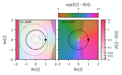
The Hartree-Fock shifted action plays an important role in achieving better series convergence in CDet. Figure 8 compares the ED analytic structure of the total energy with and without the Hartree-Fock shift. Without the shift, even for the equilibrium distance (usually considered ‘weakly correlated’), there are poles deep inside the unit circle, implying a highly divergent series at . In contrast, the Hartree-Fock shift pushes the poles away from the origin, which leads to a convergent series as seen in Fig. 4 and Fig. 6.


The CDet approach gives access to dynamic quantities, such as the Green’s function and the self-energy , through the scattering amplitude . The left column of Fig. 9 shows the CDet measurement of in Matsubara frequency space up to for , STO-6g at and . As we increase the expansion order, CDet results gradually converge to the ED solution (black lines), and at order 6 we observe only a small systematic error due to order truncation. The CDet self-energy is calculated from following Eq. (45). Both quantities exhibit similar behavior, as shown in the right column of Fig. 9. At order 3 and higher, the real part of takes non-zero value at high-frequency limit, corresponding to the correction to the frequency-independent Hartree-Fock self-energy . The CDet Green’s function, derived from following Eq. (44), is shown in Fig. 10. Good agreement with ED is observed at on the top panel, where both the Monte Carlo error estimation and the systematic error due to order truncation is much smaller than the symbol size. The bottom panel shows convergence of CDet Green’s function to ED by increasing , with a small but visible systematic deviation at low frequency when .

The generality of our CDet implementation allows a straightforward extension to much larger basis sets. Going beyond the minimal basis, we compute the CDet total energy of using cc-pVDZ and cc-pVTZ basis sets with 10 and 28 orbitals in total, respectively, and compare to the ED solution as shown in Fig. 11. For , CDet gives decent convergence to ED at , with both stochastic and systematic error below . The 2 s and 2 p orbitals added by cc-pVDZ basis and 3 s, 3 p and 3 d orbitals by cc-pVTZ basis are mostly unoccupied, and the most electron excitation occur near the lowest 1 s orbitals. Consequently, the convergence behavior and computational cost of CDet do not change significantly from the minimal basis STO-6g.

Finally, we extend our method to bigger molecules by adding more hydrogen atoms to the system. We consider a chain of 10 hydrogen atoms on a straight line with equal spacing , the same benchmark system used in Ref. Motta et al. 2017. At minimal basis STO-6g, all ten 1 s orbitals contribute equally to the active space of 10 electrons. Compared to with cc-pVDZ, which has the same number of orbitals, with STO-6g has more orbitals relevant to electron correlations, and the cost of CDet is higher (for a detailed analysis see Sec. III.2). The left column of Fig. 12 plots the CDet total energy up to in comparison to ED solution at . Convergence within is achieved at for , and systematic deviations are evident for . Similar behavior can be found in the the zero-temperature coupled cluster (CCSD) result (dotted lines), as both methods rely on the perturbative expansions of electron-electron interactions in different forms. The computational cost becomes much higher as we go to a bigger basis for . With cc-pVDZ, there are 50 atomic orbitals in total, with potential excitations to the empty orbitals from all 10 electrons. As shown in the right column Fig. 12, CDet still agrees with the reference method (MRCI+Q data from Ref. Motta et al. 2017 at ) for small values of , but the Monte Carlo errors are significantly larger. Although our generic implementation has achieved decent extensibility without fine tuning for each specific system, more efficient Monte Carlo estimators and sampling schemes as well as analytical resummation techniques should advance the limit of CDet to more complex systems.
III.2 Analysis of computational cost

The computational cost of a Markov chain Monte Carlo simulation, measured as the computational time needed for reaching a result for observable within a desired accuracy , is determined by three factors. First, the cost of each individual update, which is for a configuration at expansion order according to Algorithm 1. Second, the number of configuration updates needed to reach an independent sample by transversing a Markov chain of potentially correlated configurations, described by the integrated autocorrelation time . Finally, the variance of the estimator of the quantity of interest (Table 1), such that
| (64) |
To assess the computational cost of our CDet implementation for reaching a certain uncertainty level, as well as how the effort changes with respect to temperature, choice of basis set, and system size, we perform a series of simulations of convergent series for the hydrogen chain with the same Monte Carlo updates and measurements for a fixed number of Markov chain iterations. In Fig. 13, we show estimates of autocorrelation effects, actual computational costs, and stochastic uncertainties in total energy, as functions of temperature , the number of orbitals , or the number of hydrogen atoms in log-log plots. We rescale the -values by an arbitrary factor to emphasize the respective scaling of these quantities in the same plot.
Figure 13.a shows the temperature dependence of CDet simulations of a fixed system (, STO-6g, ) at . We observe that the simulation time does not change significantly as we decrease temperature, indicating similar distributions of the expansion order (usually tilted to the highest order). The error estimate in total energy follows almost the same tendency as the factor of the autocorrelation effect , indicating the underlying energy estimator does not have strong temperature dependence. The autocorrelation effect shows a slow power-law increase as temperature is lowered, implying that our Monte Carlo updates remain efficient at low temperature.
A similar analysis is shown in Fig. 13.b for the basis set dependence of the same system (, ) at fixed temperature. We perform CDet simulations with for basis sets STO-6g, cc-pVDZ, and cc-pVTZ, with 2, 10, and 28 atomic orbitals, respectively. As we add more ‘virtual’ orbitals to the system, the computational time increases slowly, and the autocorrelation time even decreases as the additional orbitals improve the connectivity of Monte Carlo configurations. However, the stochastic error shows a different trend from the autocorrelation effect and increases (a fit with a power law results in ), meaning that the additional orbitals introduce more diagrammatic configurations with alternating signs that lead to stronger Monte Carlo fluctuations.
As we increase the systems size in Fig. 13.c by adding more hydrogen atoms, the stochastic error (normalized by the system size ) at fixed computational time increases with a much larger power law than Fig. 13.b (fitted ), while the autocorrelation time barely changes. This implies that adding electrons that contribute to excitations near the Fermi level rapidly increases the complexity of the diagrammatics. The result is very different from the situation where additional basis states for the same number of electrons are added (Fig. 13.b).
The behavior illustrated in Fig. 13.c also differs from diagrammatic Monte Carlo applications with short-range or on-site interactions, which are formulated directly in the thermodynamic limit Prokof’ev and Svistunov 1998; Prokof’ev and Svistunov 2008a; Prokof’ev and Svistunov 2008b and usually do not show strong scaling dependencies on system size. We suspect the difference is caused by the long range nature of the bare Coulomb interaction, which introduces significant non-local electronic correlations as the system size increases. In this case, the use of ‘bold’ (or ‘screened’) interactions instead of the bare Coulomb interactions, as performed in Ref. Motta et al. 2017, may alleviate the problem. However, “bold” methods must deal with intrinsic issues of misconvergence to unphysical solutions Kozik et al. 2015. Moreover, adapting such a method to the CDet framework requires further algorithmic development. This topic is under active development Rossi et al. 2016; Rossi et al. 2020.
Thus, through the empirical analysis above, we have shown that for convergent series, the computational cost of our CDet implementation is not very sensitive to changes in temperature or basis sets, but depends strongly on the size of the system, or more specifically, on the number of valence electrons directly participating in electron excitations.
III.3 Realistic impurity: SEET for NiO
Finally, we test our CDet implementation in a general quantum impurity problem setup that includes the coupling to a non-interacting bath. We employ the SEET framework Zgid and Gull 2017 for the antiferromagnetic compound NiO, which was studied by Mott Mott 1949 as one of the original correlated insulators. Following the computational setup in Ref. Iskakov et al. 2020, we choose fcc NiO with lattice constant at temperature (). The unit cell is doubled along the direction to capture the antiferromagnetic ordering, which contains two nickel atoms and two oxygen atoms. We use a momentum discretization and the gth-dzvp-molopt-sr basis set VandeVondele and Hutter 2007 with gth-pbe pseudopotential Goedecker et al. 1996. The Coulomb integral is decomposed using density fitting with the def2-svp-ri auxiliary basis Hättig 2005. For benchmark purposes, we select the orbitals of both Ni atoms in the unit cell as the strongly correlated ‘impurities’, which is the minimal choice of impurities to capture correlation effects. This yields two independent impurities each with two orbitals. ‘Non-interacting’ impurity propagators are generated from a converged simulation of the complete unit cell following the SEET framework (for details of the computational setup see Ref. Iskakov et al. 2020).

As a benchmark, we compare our CDet impurity solver to the ED Iskakov and Danilov 2018 results used in Ref. Iskakov et al. 2020. ED requires the discretization of the continuous bath spectrum and its approximation by a few states. In order to separate ED bath fitting errors from the performance of the CDet method, we run our method for the ‘non-interacting’ impurity Green’s function corresponding to the discretized non-interacting problem solved by ED. A precise listing of all parameters and input Green’s functions is given in the supplement 11 1 See Supplemental Material at [URL will be inserted by publisher] for a precise listing of the input ‘non-interacting’ Green’s function (without Hartree-Fock contribution) and the interaction tensor defined in Appendix A. Data is stored as a comma-separated text file with explanatory headers and comments.. Figure 14 shows the impurity Green’s functions for one of the two impurities. At , the impurity Green’s function from CDet agrees with the ED solution within line width, and the stochastic uncertainty is almost invisible. The spin polarization due to the antiferromagnetic ordering is greatly enhanced in both the ED and the CDet solutions, indicating that dynamical correlations plays an important role and are well captured by the selected impurity.

In Fig. 15, we take a closer look at the convergence of CDet series in comparison to ED by plotting the differences of CDet impurity Green’s functions to ED at different order truncations up to . We observe that for both spins, the CDet result consistently converges to the ED result, giving agreement to within a percent for . The convergence of the spin down component is slower than spin up, which is consistent to what can be observed in Fig. 14, i.e. the Hartree-Fock contribution already accounts for a greater part of the overall interaction contribution for the spin up component than for spin down.
The comparison to ED illustrates that our CDet solver can be reliably applied to general impurity problems as part of a quantum embedding theory using the exact same framework as developed for molecules. We emphasize that, at the same complexity, systems with continuous bath states can be solved. Our method is therefore a controlled method for quantum impurities with general multi-orbital interactions and hybridizations, not limited by the systematic error introduced by the bath discretization procedure. The application of the solver to more complex impurities, where ED calculations are impractical, is a topic of subsequent publications.
IV Conclusion
In conclusion, we have presented a diagrammatic Monte Carlo method for quantum impurity models with general interactions and hybridizations using the connected determinant formalism Rossi 2017. We have tested the method at the example of molecular systems, which presents a systematic way of changing correlation strength, system size, basis size, and temperature. We have also tested our method for impurity problems occurring in realistic quantum impurity calculations.
Our method is formulated in the language of Green’s functions and self-energies. As a grand-canonical finite-temperature method, it is able to describe systems with particle number fluctuations and excited states. However, similar to other perturbative methods, the diagrammatic series breaks down in the strong correlation regime. This breakdown is clearly evident in the order-by-order convergence of the series and, as we have shown in detail, can be traced back to the pole structure of the diagram series.
Our method fills a crucial need of impurity solvers able to treat general four-fermion interaction and general off-diagonal hybridizations in large multi-orbital problem. It should therefore find applications in moderately correlated real-material simulations such as those occurring in DMFT Georges et al. 1996; Kotliar et al. 2006 and SEET Kananenka et al. 2015; Lan et al. 2015; Lan et al. 2016; Zgid and Gull 2017.
Further methodological progress, such as the use of higher order counterterms Rossi et al. 2020, better integration methods Maček et al. 2020, complex conformal mapping techniques Wu et al. 2017; Rossi et al. 2018; Bertrand et al. 2019b, and other types of Monte Carlo updates will expand the accessible parameter regime of the method and may make simulations in the strongly correlated regime possible.
Acknowledgements.
JL, MW, and EG were supported by the Simons Foundation as part of the Simons Collaboration on the Many-Electron Problem. During the writing phase of the paper, MW was supported by the Austrian Science Fund (FWF) through the VeCoCo project (P30997). We thank Riccardo Rossi, Fedor Šimkovic, Félix Werner, and Dominika Zgid for helpful discussions. Molecular integrals are computed using the PySCF library Sun et al. 2018. Exact diagonalization data are computed using the EDLib library Iskakov and Danilov 2018.Appendix A Hamiltonian
We describe the molecular electrons using the second quantized Hamiltonian
| (65a) | ||||
| (65b) | ||||
| (65c) | ||||
where is the electron annihilation (creation) operator associated with orbital and spin . The one- and two-body ‘matrix elements’ are defined as
| (66) | ||||
| (67) |
where are the coordinates of the nuclei, each with charge , and is the electron mass. Eq. (65) defines a quantum many-body problem which can be studied with a wide range of approximate or exact theoretical and numerical methods.
Appendix B Scattering amplitude
The intuition in defining the object is similar to the relation between the self-energy and the Luttinger-Ward functional
| (71) |
which gives the 1PI amputated diagrams with the ‘bold’ propagator Luttinger and Ward 1960. Here we have employed the compound space-time indices . To get the connected amputated diagrams with the ‘bare’ propagator instead, we define a similar relation
| (72) |
We show that by carrying out this functional derivative, we will recover the definition of as in Eq. (20).
Switching to the action formalism using coherent state path-integrals of Grassmann variables Negele and Orland 1988, we rewrite the partition function as
| (73) |
where the action is given as
| (74) |
Observe that
| (75) |
Using the fact that for an invertible matrix ,
| (76) | |||
| (77) |
we have
| (78) |
Similarly in the non-interacting case,
| (79) |
Putting it all together, we have
| (80) |
Therefore
| (81) |
which is exactly the same as Eq. (20).
Appendix C Thermal expectation value of the electron energy
The one-body energy is straightforward:
| (86) |
Expression for the two-body energy term can be derived in multiple ways such as using the equation of motion or the Schwinger-Dyson equation. Here we provide a simple derivation following Ref. Lin and Lindsey 2018. We introduce a coupling constant to the action defined in Eq. (74) such that and recovers the ‘physical’ results. Now we have
| (87) |
Introducing a change of variables such that and , then
| (88) |
where the indices denote states at each discretized time point on the integration path, in which is the compound spacetime index, and the plus sign on the exponent is due to the nature of Grassmann integrals. The partition function is unaffected by the change of variables, which now takes the form
| (89) |
Therefore
| (90) |
Comparing (87) and (90), we have
| (91) |
Appendix D Recursion relations for the grand potential
The expansion of the grand potential, Eq. (16), consists of connected vacuum diagrams as shown in Fig. 1. As a result of Wick’s theorem (10), all vacuum diagrams for a fixed vertex configuration can be partitioned into a connected subdiagram and the remainder of the vacuum components. Since no external legs exist to serve as reference points for defining connectivity, we start by picking a specific vertex as the ‘reference’ and consider connectivity with respect to , i.e.
| (92) |
As the choice of is arbitrary, it can be any of the vertices in , therefore
| (93) |
This is equivalent to iterating all possible subsets of where the reference can be any vertex in :
| (94) |
We now extract the term where from the right hand side and obtain the recursive formula for :
| (95) |
The initial condition is the zeroth order contribution .
A more general framework of deriving the recursion relations using idempotent polynomials is described in Ref. Rossi 2018. This framework does not resort to topological arguments.
Appendix E Numerical computation of the adjugate matrix
We calculate the adjugate of a matrix numerically by first performing a rank-revealing factorization on the matrix Stewart 1998, such as the pivoted QR via the Householder algorithm
| (96) |
where is an orthogonal matrix of Householder reflections, is a diagonal matrix, is an upper triangular matrix in which all diagonal elements equal 1, and is a permutation matrix of the columns. The rank of the matrix is determined by the number of nonzero diagonal elements of .
If is not singular, i.e. , then the adjugate is given by
| (97) |
where is the number of transpositions in the permutation , is the number of Householder reflections in , and are diagonal elements of . The scaling as a function of for the complexity of calculating the adjugate is the same as the one for calculating , and we obtain at the same time.
If is singular, i.e. , becomes zero, and Eq. (97) is replaced by
| (98) |
If , there is one zero in the diagonal of . Assuming and for , the adjugate of follows directly from the definition (23)
| (99) |
If , , therefore .
In the presence of off-diagonal propagators, it is possible that the amputated diagrams is nonzero while the vacuum diagrams vanish. Therefore it is crucial to implement the adjugate of singular matrices as discussed above.
References
- Anderson (1961) P. W. Anderson, Phys. Rev. 124, 41 (1961).
- Hanson et al. (2007) R. Hanson, L. P. Kouwenhoven, J. R. Petta, S. Tarucha, and L. M. K. Vandersypen, Reviews of Modern Physics 79, 1217 (2007).
- Brako and Newns (1981) R. Brako and D. M. Newns, Journal of Physics C: Solid State Physics 14, 3065 (1981).
- Langreth and Nordlander (1991) D. C. Langreth and P. Nordlander, Phys. Rev. B 43, 2541 (1991).
- Georges et al. (1996) A. Georges, G. Kotliar, W. Krauth, and M. J. Rozenberg, Reviews of Modern Physics 68, 13 (1996).
- Kotliar et al. (2006) G. Kotliar, S. Y. Savrasov, K. Haule, V. S. Oudovenko, O. Parcollet, and C. A. Marianetti, Reviews of Modern Physics 78, 865 (2006).
- Lichtenstein and Katsnelson (2000) A. I. Lichtenstein and M. I. Katsnelson, Phys. Rev. B 62, R9283(R) (2000).
- Kotliar et al. (2001) G. Kotliar, S. Y. Savrasov, G. Pálsson, and G. Biroli, Phys. Rev. Lett. 87, 186401 (2001).
- Hettler et al. (2000) M. H. Hettler, M. Mukherjee, M. Jarrell, and H. R. Krishnamurthy, Phys. Rev. B 61, 12739 (2000).
- Maier et al. (2005) T. Maier, M. Jarrell, T. Pruschke, and M. H. Hettler, Rev. Mod. Phys. 77, 1027 (2005).
- Anisimov et al. (1997) V. I. Anisimov, A. I. Poteryaev, M. A. Korotin, A. O. Anokhin, and G. Kotliar, Journal of Physics: Condensed Matter 9, 7359 (1997).
- Lichtenstein and Katsnelson (1998) A. I. Lichtenstein and M. I. Katsnelson, Physical Review B 57, 6884 (1998).
- Held et al. (2006) K. Held, I. A. Nekrasov, G. Keller, V. Eyert, N. Blümer, A. K. McMahan, R. T. Scalettar, T. Pruschke, V. I. Anisimov, and D. Vollhardt, physica status solidi (b) 243, 2599 (2006).
- Sun and Kotliar (2002) P. Sun and G. Kotliar, Physical Review B 66, 085120 (2002).
- Biermann et al. (2003) S. Biermann, F. Aryasetiawan, and A. Georges, Physical Review Letters 90, 086402 (2003).
- Biermann et al. (2005) S. Biermann, F. Aryasetiawan, and A. Georges, in Physics of Spin in Solids: Materials, Methods and Applications, edited by S. Halilov (Springer Netherlands, Dordrecht, 2005) pp. 43–65.
- Boehnke et al. (2016) L. Boehnke, F. Nilsson, F. Aryasetiawan, and P. Werner, Physical Review B 94, 201106(R) (2016).
- Choi et al. (2016) S. Choi, A. Kutepov, K. Haule, M. van Schilfgaarde, and G. Kotliar, npj Quantum Materials 1, 16001 (2016).
- Lee and Haule (2017) J. Lee and K. Haule, Phys. Rev. B 95, 155104 (2017).
- Kananenka et al. (2015) A. A. Kananenka, E. Gull, and D. Zgid, Physical Review B 91, 121111(R) (2015).
- Lan et al. (2015) T. N. Lan, A. A. Kananenka, and D. Zgid, The Journal of Chemical Physics 143, 241102 (2015).
- Lan et al. (2016) T. N. Lan, A. A. Kananenka, and D. Zgid, Journal of Chemical Theory and Computation 12, 4856 (2016).
- Zgid and Gull (2017) D. Zgid and E. Gull, New Journal of Physics 19, 023047 (2017).
- Mazurenko et al. (2010) V. V. Mazurenko, S. N. Iskakov, A. N. Rudenko, V. I. Anisimov, and A. I. Lichtenstein, Phys. Rev. B 82, 193403 (2010).
- Caffarel and Krauth (1994) M. Caffarel and W. Krauth, Phys. Rev. Lett. 72, 1545 (1994).
- Capone et al. (2004) M. Capone, M. Civelli, S. S. Kancharla, C. Castellani, and G. Kotliar, Phys. Rev. B 69, 195105 (2004).
- Koch et al. (2008) E. Koch, G. Sangiovanni, and O. Gunnarsson, Phys. Rev. B 78, 115102 (2008).
- Liebsch and Tong (2009) A. Liebsch and N.-H. Tong, Phys. Rev. B 80, 165126 (2009).
- Sénéchal (2010) D. Sénéchal, Phys. Rev. B 81, 235125 (2010).
- Lu et al. (2014) Y. Lu, M. Höppner, O. Gunnarsson, and M. W. Haverkort, Phys. Rev. B 90, 085102 (2014).
- Zgid et al. (2012) D. Zgid, E. Gull, and G. K.-L. Chan, Phys. Rev. B 86, 165128 (2012).
- Shee and Zgid (2019) A. Shee and D. Zgid, Journal of Chemical Theory and Computation 15, 6010 (2019), pMID: 31518129.
- Zhu et al. (2019) T. Zhu, C. A. Jiménez-Hoyos, J. McClain, T. C. Berkelbach, and G. K.-L. Chan, Phys. Rev. B 100, 115154 (2019).
- Weichselbaum and von Delft (2007) A. Weichselbaum and J. von Delft, Phys. Rev. Lett. 99, 076402 (2007).
- Bulla et al. (2008) R. Bulla, T. A. Costi, and T. Pruschke, Rev. Mod. Phys. 80, 395 (2008).
- Gull et al. (2011a) E. Gull, A. J. Millis, A. I. Lichtenstein, A. N. Rubtsov, M. Troyer, and P. Werner, Reviews of Modern Physics 83, 349 (2011a).
- Rubtsov et al. (2005) A. N. Rubtsov, V. V. Savkin, and A. I. Lichtenstein, Physical Review B 72, 035122 (2005).
- Gull et al. (2008) E. Gull, P. Werner, O. Parcollet, and M. Troyer, EPL (Europhysics Letters) 82, 57003 (2008).
- Gull et al. (2011b) E. Gull, P. Staar, S. Fuchs, P. Nukala, M. S. Summers, T. Pruschke, T. C. Schulthess, and T. Maier, Phys. Rev. B 83, 075122 (2011b).
- LeBlanc et al. (2015) J. P. F. LeBlanc, A. E. Antipov, F. Becca, I. W. Bulik, G. K.-L. Chan, C.-M. Chung, Y. Deng, M. Ferrero, T. M. Henderson, C. A. Jiménez-Hoyos, E. Kozik, X.-W. Liu, A. J. Millis, N. V. Prokof’ev, M. Qin, G. E. Scuseria, H. Shi, B. V. Svistunov, L. F. Tocchio, I. S. Tupitsyn, S. R. White, S. Zhang, B.-X. Zheng, Z. Zhu, and E. Gull (Simons Collaboration on the Many-Electron Problem), Phys. Rev. X 5, 041041 (2015).
- Gorelov et al. (2009) E. Gorelov, T. O. Wehling, A. N. Rubtsov, M. I. Katsnelson, and A. I. Lichtenstein, Phys. Rev. B 80, 155132 (2009).
- Werner et al. (2006) P. Werner, A. Comanac, L. de’ Medici, M. Troyer, and A. J. Millis, Phys. Rev. Lett. 97, 076405 (2006).
- Werner and Millis (2006) P. Werner and A. J. Millis, Phys. Rev. B 74, 155107 (2006).
- Haule (2007) K. Haule, Phys. Rev. B 75, 155113 (2007).
- Eidelstein et al. (2019) E. Eidelstein, E. Gull, and G. Cohen, arXiv:1907.08570 [cond-mat.str-el] (2019).
- Cohen et al. (2015) G. Cohen, E. Gull, D. R. Reichman, and A. J. Millis, Phys. Rev. Lett. 115, 266802 (2015).
- Prokof’ev and Svistunov (1998) N. V. Prokof’ev and B. V. Svistunov, Physical Review Letters 81, 2514 (1998).
- Prokof’ev and Svistunov (2008a) N. Prokof’ev and B. Svistunov, Physical Review B 77, 020408(R) (2008a).
- Prokof’ev and Svistunov (2008b) N. V. Prokof’ev and B. V. Svistunov, Physical Review B 77, 125101 (2008b).
- van Houcke et al. (2010) K. van Houcke, E. Kozik, N. Prokof’ev, and B. Svistunov, Physics Procedia 6, 95 (2010), computer Simulations Studies in Condensed Matter Physics XXI.
- Chen and Haule (2019) K. Chen and K. Haule, Nature Communications 10, 3725 (2019).
- Rossi (2017) R. Rossi, Physical Review Letters 119, 045701 (2017).
- Rossi (2018) R. Rossi, arXiv:1802.04743 [cond-mat.str-el] (2018).
- Boag et al. (2018) A. Boag, E. Gull, and G. Cohen, Phys. Rev. B 98, 115152 (2018).
- Rossi et al. (2020) R. Rossi, F. Simkovic, and M. Ferrero, arXiv:2001.09133 [cond-mat.str-el] (2020).
- Moutenet et al. (2018) A. Moutenet, W. Wu, and M. Ferrero, Physical Review B 97, 085117 (2018).
- Šimkovic and Kozik (2019) F. Šimkovic and E. Kozik, Physical Review B 100, 121102 (2019).
- Iskakov et al. (2020) S. Iskakov, C.-N. Yeh, E. Gull, and D. Zgid, Ab-initio self-energy embedding for the photoemission spectra of nio and mno (2020), arXiv:2003.04440 [cond-mat.str-el] .
- Motta et al. (2017) M. Motta, D. M. Ceperley, G. K.-L. Chan, J. A. Gomez, E. Gull, S. Guo, C. A. Jiménez-Hoyos, T. N. Lan, J. Li, F. Ma, A. J. Millis, N. V. Prokof’ev, U. Ray, G. E. Scuseria, S. Sorella, E. M. Stoudenmire, Q. Sun, I. S. Tupitsyn, S. R. White, D. Zgid, and S. Zhang, Physical Review X 7, 031059 (2017).
- Abrikosov et al. (1965) A. A. Abrikosov, L. P. Gorkov, and I. Y. Dzyaloshinskii, Methods of Quantum Field Theory in Statistical Physics (Pergamon, 1965).
- Negele and Orland (1988) J. W. Negele and H. Orland, Quantum Many-particle Systems (Addison-Wesley, 1988).
- Rossi, R. et al. (2017) Rossi, R., Prokof’ev, N., Svistunov, B., Van Houcke, K., and Werner, F., EPL 118, 10004 (2017).
- Bertrand et al. (2019a) C. Bertrand, O. Parcollet, A. Maillard, and X. Waintal, Phys. Rev. B 100, 125129 (2019a).
- Gunacker et al. (2015) P. Gunacker, M. Wallerberger, E. Gull, A. Hausoel, G. Sangiovanni, and K. Held, Phys. Rev. B 92, 155102 (2015).
- Rossi et al. (2016) R. Rossi, F. Werner, N. V. Prokof’ev, and B. Svistunov, Physical Review B 93, 161102(R) (2016).
- Hehre et al. (1969) W. J. Hehre, R. F. Stewart, and J. A. Pople, The Journal of Chemical Physics 51, 2657 (1969).
- Szabo and Ostlund (2012) A. Szabo and N. S. Ostlund, Modern quantum chemistry: introduction to advanced electronic structure theory (Courier Corporation, 2012).
- Knowles et al. (1985) P. Knowles, K. Somasundram, N. Handy, and K. Hirao, Chemical Physics Letters 113, 8 (1985).
- Olsen et al. (1996) J. Olsen, O. Christiansen, H. Koch, and P. Jørgensen, Journal of Chemical Physics 105, 5082 (1996).
- Hirata et al. (2015) S. Hirata, M. R. Hermes, J. Simons, and J. V. Ortiz, Journal of Chemical Theory and Computation 11, 1595 (2015).
- Hirata et al. (2017) S. Hirata, A. E. Doran, P. J. Knowles, and J. V. Ortiz, The Journal of Chemical Physics 147, 044108 (2017).
- Li (2019) Z. Li, The Journal of Chemical Physics 151, 244114 (2019).
- Kozik et al. (2015) E. Kozik, M. Ferrero, and A. Georges, Phys. Rev. Lett. 114, 156402 (2015).
- Mott (1949) N. F. Mott, Proceedings of the Physical Society. Section A 62, 416 (1949).
- VandeVondele and Hutter (2007) J. VandeVondele and J. Hutter, The Journal of Chemical Physics 127, 114105 (2007).
- Goedecker et al. (1996) S. Goedecker, M. Teter, and J. Hutter, Phys. Rev. B 54, 1703 (1996).
- Hättig (2005) C. Hättig, Phys. Chem. Chem. Phys. 7, 59 (2005).
- Iskakov and Danilov (2018) S. Iskakov and M. Danilov, Computer Physics Communications 225, 128 (2018).
- (79) See Supplemental Material at [URL will be inserted by publisher] for a precise listing of the input ‘non-interacting’ Green’s function (without Hartree-Fock contribution) and the interaction tensor defined in Appendix A. Data is stored as a comma-separated text file with explanatory headers and comments.
- Maček et al. (2020) M. Maček, P. T. Dumitrescu, C. Bertrand, B. Triggs, O. Parcollet, and X. Waintal, arXiv:2002.12372 [cond-mat.str-el] (2020).
- Wu et al. (2017) W. Wu, M. Ferrero, A. Georges, and E. Kozik, Phys. Rev. B 96, 041105 (2017).
- Rossi et al. (2018) R. Rossi, T. Ohgoe, K. van Houcke, and F. Werner, Phys. Rev. Lett. 121, 130405 (2018).
- Bertrand et al. (2019b) C. Bertrand, S. Florens, O. Parcollet, and X. Waintal, Phys. Rev. X 9, 041008 (2019b).
- Sun et al. (2018) Q. Sun, T. C. Berkelbach, N. S. Blunt, G. H. Booth, S. Guo, Z. Li, J. Liu, J. D. McClain, E. R. Sayfutyarova, S. Sharma, S. Wouters, and G. K. L. Chan, Wiley Interdisciplinary Reviews: Computational Molecular Science 8, e1340 (2018).
- Luttinger and Ward (1960) J. M. Luttinger and J. C. Ward, Phys. Rev. 118, 1417 (1960).
- Lin and Lindsey (2018) L. Lin and M. Lindsey, arXiv:1809.02900 (2018).
- Stewart (1998) G. W. Stewart, Linear Algebra and its Applications 283, 151 (1998).