Statistical Queries and Statistical Algorithms: Foundations and Applications This survey was first given as a tutorial on statistical queries at the 29th International Conference on Algorithmic Learning Theory (ALT) Janoos et al. 2018. Since then, various researchers have asked about the tutorial slides or noted the slides’ usefulness in helping them to absorb or teach this material. Hence, that tutorial has been developed into this survey paper in hopes that it will serve as a useful primer on this subject. To give proper attention to all of the authors of the various results, full author lists for the cited papers were provided en lieu of the customary et al. abbreviation.

Lev Reyzin Affiliation: Department of Mathematics, Statistics, and Computer Science Affiliation: University of Illinois at Chicago Email: lreyzin@uic.edu

Abstract

We give a survey of the foundations of statistical queries and their many applications to other areas. We introduce the model, give the main definitions, and we explore the fundamental theory statistical queries and how how it connects to various notions of learnability. We also give a detailed summary of some of the applications of statistical queries to other areas, including to optimization, to evolvability, and to differential privacy.

1 Introduction

Over 20 years ago, Kearns 1998 introduced statistical queries as a framework for designing machine learning algorithms that are tolerant to noise. The statistical query model restricts a learning algorithm to ask certain types of queries to an oracle that responds with approximately correct answers. This framework has has proven useful, not only for designing noise-tolerant algorithms, but also for its connections to other noise models, for its ability to capture many of our current techniques, and for its explanatory power about the hardness of many important problems.

Researchers have also found many connections between statistical queries and a variety of modern topics, including to evolvability, differential privacy, and adaptive data analysis. Statistical queries are now both an important tool and remain a foundational topic with many important questions. The aim of this survey is to illustrate these connections and bring researchers to the forefront of our understanding of this important area.

We begin by formally introducing the model and giving the main definitions (Section 2), we then move to exploring the fundamental theory of learning statistical queries and how how it connects to other notions of learnability (Section 3). Finally, we explore many of the other applications of statistical queries, including to optimization, to evolvability, and to differential privacy (Section 4).

2 Model, definitions, and basic results

Statistical query learning traces its origins to the Probably Approximately Correct (PAC) learning model of Valiant 1984. The PAC model defines the basic supervised learning framework used in machine learning. We begin with its definition.

Definition 1 (efficient PAC learning).

Let $C$ be a class of boolean functions $c:X\rightarrow\{-1,1\}$ . We say that $C$ is efficiently PAC-learnable if there exists an algorithm $\mathcal{A}$ such that for every $c\in C$ , any probability distribution $D_{X}$ over $X$ , and any $0<\epsilon,\delta<1$ , $\mathcal{A}$ takes a labeled sample $S$ of size $m=\mathrm{poly}(1/\epsilon,1/\delta,n,|c|)$ from¹¹ 1 $n=|x|$ $D$ , outputs a hypothesis $h$ for which

\mathbf{Pr}_{S\sim D}[\mathrm{err}_{D}(h)\leq\epsilon]\geq 1-\delta

in time polynomial in $m$ .

A useful way to think about the statistical query (SQ) framework is as a restriction on the algorithm $\mathcal{A}$ in the definition above. In the SQ model, the learner access to an oracle instead of to a set $S$ of labeled examples.

The oracle accepts query functions and tolerances, which together are called a statistical query. To define the model, we first make this notion presice.

Definition 2 (statistical query).

A statistical query is a pair $(q,\tau)$ with

$q$ :

a function $q:X\times\{-1,1\}\rightarrow\{-1,1\}$ .
$\tau$ :

a tolerance parameter $\tau\geq 0$ .

Now we are ready to define the statistical query oracle.

Definition 3 (statistical query oracle).

The statistical query oracle, SQ $(q,\tau)$ , when given a statistical query, returns any value in the range:

\left[\mathbf{E}_{x\sim D}[q(x,c(x)]-\tau,\mathbf{E}_{x\sim D}[q(x,c(x)]+\tau\right].

Finally, we can give the definition of efficient statistical query learning.

Definition 4 (efficient SQ learning).

Let $C$ be a class of boolean functions $c:X\rightarrow\{-1,1\}$ . We say that $C$ is efficiently SQ-learnable if there exists an algorithm $\mathcal{A}$ such that for every $c\in C$ , any probability distribution $D$ , and any $\epsilon>0$ , there is a polynomial $p(\cdot,\cdot,\cdot)$ such that

1.

$\mathcal{A}$ makes at most $p(1/\epsilon,n,|c|)$ calls to the SQ oracle,
2.

the smallest $\tau$ that $\mathcal{A}$ uses satisfies ${1}/{\tau}\leq p(1/\epsilon,n,|c|)$ , and
3.

the queries $q$ are evaluable in time $p(1/\epsilon,n,|c|)$ ,

and $\mathcal{A}$ outputs a hypothesis $h$ satisfying err ${}_{D}(h)\leq\epsilon$ .

Note that unlike Definition 1, this definition has no failure parameter $\delta$ . That is because in PAC learning, it is possible to get an uninformative sample, whereas the SQ oracle is restricted to always answer queries within a given range.

2.1 Simulating by algorithms that draw a sample

It is not hard to see that a statistical query algorithm can be simulated in the PAC model, which makes SQ a natural restriction of PAC. In particular one can simulate an SQ oracle in the PAC model by drawing $m=O\left(\frac{\log(k/\delta)}{\tau^{2}}\right)$ samples for each of the $k$ statistical queries, and by the Hoeffding bound, the simulation will fail with probability $<\delta$ . This leads to the following observation.

Observation 5.

If a class of functions is efficiently SQ-learnable, then it is efficiently PAC learnable.

More importantly, learnability with statistical queries is also related to learnability under the classification noise model of Angluin and Laird 1987.

Definition 6 (classification noise).

A PAC learning algorithm under random classification noise must meet the PAC requirements, but the label of each training sample is flipped with independently with probability $\eta$ , for $0\leq\eta<1/2$ . The sample size and running time must also depend polynomially on $1/(1-2\eta)$ .

This leads us to the following surprising theorem, which shows that any statistical query algorithm can be converted into a PAC algorithm under classification noise.

Theorem 7 (Kearns 1998).

If a class of functions is efficiently SQ-learnable, then it is efficiently learnable in the noisy PAC model.

Proof.

For each of $k$ queries, $q(.,.)$ , with tolerance $\tau$ , let Let $P=\mathbf{E}_{x\sim D}[q(x,c(x))]$ . We estimate $P$ with $\hat{P}$ as follows.

First, draw a sample set $S$ , with $|S|=\mathrm{poly}\left({1}/{\tau},{1}/{1-2\eta},\log{1}/{\delta},\log k\right)$ sufficing. Given $q$ , we separate $S$ into two parts²² 2 Note that this does not require knowing the labels of the examples.:

	$\displaystyle S_{\mathrm{clean}}=$	$\displaystyle\ \{x\in S\ \|\ q(x,0)=q(x,1)\}$
	$\displaystyle S_{\mathrm{noisy}}=$	$\displaystyle\ \{x\in S\ \|\ q(x,0)\neq q(x,1)\}.$

Then, we estimate $q$ on both the parts, with

	$\displaystyle\hat{P}_{\mathrm{clean}}=$	$\displaystyle\ \frac{\sum_{x\in S_{\mathrm{clean}}}q(x,\ell(x))}{\left\|S_{\mathrm{clean}}\right\|}$
	$\displaystyle\hat{P}_{\mathrm{noisy}}=$	$\displaystyle\ \frac{\sum_{x\in S_{\mathrm{noisy}}}q(x,\ell(x))}{\left\|S_{\mathrm{noisy}}\right\|}.$

Finally, since we know the noise rate $\eta$ , we can undo the noise on the noisy part and combine the estimate:

\hat{P}=\frac{\hat{P}_{\mathrm{noisy}}-\eta}{1-2\eta}\left(\frac{|S_{\mathrm{noisy}}|}{|S|}\right)+\hat{P}_{\mathrm{clean}}\left(\frac{|S_{\mathrm{clean}}|}{|S|}\right).

By the Hoeffding and union bound, we can show that $\hat{P}$ is within $\tau$ of $P$ with probability at least $1-\delta$ for all $k$ queries for the $|S|$ as chosen above. ∎

Therefore, the SQ framework gives us a way to design algorithms that are also noise-tolerant under some notions of noise. In addition, SQ learnability also gives results for learning in the malicious noise model of Valiant 1985, for example as illustrated in the following Theorem.

Theorem 8 (Aslam and Decatur 1998a).

If a class of functions is efficiently SQ-learnable, then it is efficiently PAC learnable under malicious noise with noise rate $\eta=\tilde{O}(\epsilon)$ .

2.2 Variants of SQs

One natural restriction of statistical queries was defined by Bshouty and Feldman 2002, who modified the oracle to only output the approximate correlation between a query and the target function. In this correlational statistical query (CSQ) model, the oracle is weaker, but the learning criterion is the same as for statistical queries, as in Definition 4.

Definition 9 (correlational statistical query oracle).

Given a function $h=X\rightarrow\{-1,1\}$ and a tolerance parameter $\tau$ , the correlational statistical query oracle CSQ $(h,\tau)$ returns a value in the range

[\mathbf{E}_{D}[h(x)c(x)]-\tau,\mathbf{E}_{D}[h(x)c(x)]+\tau].

The correlational statistical query oracle above gives distances between the hypothesis and a target function. This is equivalent to the “Learning by Distances” model of Ben-David et al. 1995, who defined their model independently of Kearns 1998.

Another natural way to define statistical queries presented by Yang 2005 is via the honest statistical query (HSQ) oracle. This oracle samples the distribution and honestly computes approximate answers.

Definition 10 (honest statistical query oracle).

Given function $q:X\times\{-1,1\}\rightarrow\{-1,1\}$ and sample size $m$ , the honest statistical query oracle HSQ $(q,s)$ draws $\left(x_{1},\ldots,x_{m}\right)\sim D^{m}$ and returns the empirical average

\frac{1}{m}\sum_{i=1}^{m}q(x_{i},c(x_{i})).

The definition of honest statistical query learning is again similar to Definition 4, but needs some modification to work with the HSQ oracle. First, instead of bounding $1/\tau$ , the largest sample size $m$ needs to be bounded by a polynomial. Also, because of the sampling procedure, a failure parameter $\delta$ needs to be (re-)introduced, and the learner is required to also be polynomial in ${1}/{\delta}$ .

Note that because the CSQ oracle is weaker, any lower bound against SQ algorithms also holds against CSQ algorithms. On the other hand, the HSQ oracle is arguably stronger and cannot answer adversarially; hence, SQ algorithms can be easily adapted to give HSQ guarantees.

3 Bounds for SQ algorithms

We now examine some fundamental theory for statistical query algorithms, beginning with information-theoretic lower bounds that hold against statistical query algorithms.

3.1 Lower bounds

The main tool for proving statistical query lower bounds is called statistical query dimension. We present it and variants of it in the following section.

3.1.1 Statistical query dimension

A quantity called the statistical query dimension [Blum et al. 1994] controls the complexity of statistical query learning.

Definition 11 (statistical query dimension).

For a concept class $C$ and distribution $D$ , the statistical query dimension of $C$ with respect to $D$ , denoted $\mathrm{SQ\mbox{-}DIM}_{D}(C)$ , is the largest number $d$ such that $C$ contains $d$ functions $f_{1},f_{2},\ldots,f_{d}$ such that for all $i\neq j,$ $\left|\left<f_{i},f_{j}\right>_{D}\right|\leq 1/d.$ Note: $\left<f_{i},f_{j}\right>_{D}=\mathbf{E}_{D}[f_{i}\cdot f_{j}].$

When we leave out the distribution $D$ as a subscript, we refer to the statistical query dimension with respect to the worst-case distribution

\mathrm{SQ\mbox{-}DIM}(C)=\max_{D\in\mathcal{D}}\left(\mathrm{SQ\mbox{-}DIM}_{D}(C)\right).

This quantity is important due to the following theorem.

Theorem 12 (Blum et al. 1994).

Let $C$ be a concept class and let $d=\mathrm{SQ\mbox{-}DIM}_{D}(C)$ . Then any SQ learning algorithm that uses a tolerance parameter lower bounded by $\tau>0$ must make at least $(d\tau^{2}-1)/2$ queries to learn $C$ with accuracy at least $\tau$ . In particular, when $\tau=1/d^{1/3}$ , this means $(d^{1/3}-1)/2$ queries are needed.

Proof.

The original proof is a bit too technical to present here, so instead we’ll see a clever, short proof of this lower bound for CSQs given by Szörényi 2009. This proof gives a weaker result than the statement of the theorem as proven by Blum et al. 1994.

Assume $f_{1},\ldots,f_{d}$ realize the SQ-DIM. Let $h$ be a query and $A=\{i\in[d]:\left<f_{i},h\right>\geq\tau\}$ . Then by Cauchy-Schwartz, we have

\left<h,\sum_{i\in A}f_{i}\right>^{2}\leq\left|\left|\sum_{i\in A}f_{i}\right|\right|^{2}=\sum_{i,j\in A}\left<f_{i},f_{j}\right>\leq\sum_{i\in A}\left(1+\frac{|A|-1}{d}\right)

(1)

therefore

\left<h,\sum_{i\in A}f_{i}\right>^{2}\leq|A|+\frac{|A|^{2}}{d}.

But by definition of $A$ , we also have

\left<h,\sum_{i\in A}f_{i}\right>\geq|A|\tau.

By algebra, $|A|\leq d/(d\tau^{2}-1)$ , and the same bound holds for $A^{\prime}$ defined with respect to correlation $\leq-\tau$ .

So, no matter what $h$ is asked of the oracle, an answer of $0$ to CSQ $(h,\tau)$ is inconsistent with at most $|A|+|A^{\prime}|\leq 2d/(d\tau^{2}-1)$ of the functions $f_{i}$ . Since $d$ (or, technically, $d-1$ ) functions need to be eliminated, this implies the desired lower bound. ∎

We then get the following as an immediate corollary.

Corollary 13.

Let $C$ be a class with $\mathrm{SQ\mbox{-}DIM}_{D}(C)=\omega(n^{k})$ for all $k$ , then $C$ is not efficiently SQ-learnable under $D$ .

Perhaps surprisingly, for distribution-specific learning, CSQ-learnability is equivalent to SQ-learnability.

Lemma 14 (Bshouty and Feldman 2002).

Any SQ can be answered by asking two SQs that are independent of the target and two CSQs.

Proof.

We decompose the SQ into two SQs:

$\displaystyle\mathbf{E}_{D}[q(x,c(x)]=$	$\displaystyle\ \mathbf{E}_{D}\left[q(x,-1)\frac{1-c(x)}{2}+q(x,1)\frac{1+c(x)}{2}\right]$
$\displaystyle=$	$\displaystyle\ \frac{1}{2}\mathbf{E}_{D}[q(x,1)c(x)]\ -\ \frac{1}{2}\mathbf{E}_{D}[q(x,-1)c(x)]\ +$	(2)
	$\displaystyle\ \frac{1}{2}\mathbf{E}_{D}[q(x,1)]\ +\ \frac{1}{2}\mathbf{E}_{D}[q(x,-1)].$	(3)

Note that the terms in Expression 2 are correlational statistical queries and the terms in Expression 3 are statistical queries independent of the label. ∎

On the other hand, Feldman 2011 showed that CSQs are strictly weaker than SQs for distribution-independent learning. For example, he showed that half-spaces are not distribution-independently CSQ learnable, but are SQ learnable.

There also exists a similar theorem for honest statistical queries, as given below. The statement was originally proven by Yang 2005 and later strengthened by Feldman et al. 2017.

Theorem 15 (Yang 2005).

Let $C$ be a concept class and let $d=\mathrm{SQ\mbox{-}DIM}(C)$ . Then any HSQ learning algorithm must use a total sample complexity at least $\Omega(d)$ to learn $C$ to constant accuracy and probability of success.

3.1.2 Classes that are not efficiently SQ learnable

Given the statistical query dimension lower bounds, we can now say certain classes of functions are not learnable with statistical queries, begging with a result from the results in the original paper of Kearns 1998.

Observation 16.

Parity functions on $\{0,1\}^{n}$ have $\mathrm{SQ\mbox{-}DIM}=2^{n}$ , and therefore, are not efficiently SQ learnable.

Parity functions are of the form $\chi_{c}(x)=(-1)^{c\cdot x}$ . All $2^{n}$ of them are pairwise orthogonal. This is known from orthogonality of Fourier characters under the uniform distribution; see the book by O’Donnell 2014. Parities, however, being linear functions, are PAC-learnable using Gaussian elimination, so SQ $\subsetneq$ PAC. [Blum et al. 1994].

Observation 17.

Decision trees on $n$ nodes have $\mathrm{SQ\mbox{-}DIM}\geq n^{c\log n}$ , and therefore, are not efficiently SQ learnable.

This fact can be proven by showing how decision trees can encode many parity functions, all of which are pairwise orthogonal. This is the standard technique for showing a high statistical query dimension.

Refer to caption — Figure 1: A decision tree on $7$ nodes encoding the parity function on $3$ variables.

Figure 1 illustrates the straightforward way how a decision tree with $n-1$ nodes can encode a parity function on $\log n$ variables. Since there are $\binom{n}{\log n}$ choices of $\log n$ from $n$ variables, this shows decision trees have a statistical query dimension of at least $n^{c\log n}$ .

Observation 18.

DNF of size n have $\mathrm{SQ\mbox{-}DIM}\geq n^{c\log n}$ , and therefore, are not efficiently SQ learnable.

$(x_{1}\wedge x_{2}\wedge x_{3})\vee(\bar{x}_{1}\wedge\bar{x}_{2}\wedge\bar{x}_{3})\vee(\bar{x}_{1}\wedge{x}_{2}\wedge\bar{x}_{3})\vee(\bar{x}_{1}\wedge\bar{x}_{2}\wedge{x}_{3})$

Figure 2: A

4

-term DNF encoding the parity function on

3

variables

DNF formulae of size $n$ can similarly encore parity functions on $\log n$ variables using $n/2$ terms, as illustrated in Figure 2.

Observation 19.

Deterministic finite automata on $n$ nodes have $\mathrm{SQ\mbox{-}DIM}\geq 2^{cn}$ , and therefore, are not efficiently SQ learnable.

Figure 3 illustrates how deterministic finite automaton with $2n+1$ nodes can encode a parity function on $n$ variables. Note that the crossings correspond to variables relevant to the parity function.

It turns out that even uniformly random decision trees, DNF, and automata [Angluin et al. 2010].

Note that only the first of these are known to be PAC learnable. We will discuss the implications of this in Section 3.3.

3.1.3 Comparison with VC dimension

The results above imply certain relationships to other notions of dimension. In this section, we briefly explore the relationship of $\mathrm{SQ\mbox{-}DIM}$ with the Vapnik-Chervonenkis dimension, $\mathrm{VC\mbox{-}DIM}$ , which controls the sample complexity of PAC learning [Vapnik and Chervonenkis 2015]. Briefly stated, the $\mathrm{VC\mbox{-}DIM}$ of a concept class $\mathcal{C}$ is the maximum number of examples that $C$ can shatter, i.e. achieve all possible labelings of the examples by functions in $C$ .

First, we make the following observation, which also appears in Blum et al. 1994

Observation 20.

For a concept class $C$ , let $\mathrm{VC\mbox{-}DIM}(C)=d$ , then $\mathrm{SQ\mbox{-}DIM}(C)=\Omega(d)$ .

Proof.

Let $d$ be the VC dimension of $C$ . Then there exists a set $S$ of $d$ points $C$ can shatter. Assume without loss of generality that the domain of $S$ is $\{0,1\}^{\log d}$ . Because $C$ shatters $S$ , it contains all $d$ parity functions over $\{0,1\}^{\log d}$ , which by Observation 16 have $\mathrm{SQ\mbox{-}DIM}$ of $2^{\log d}=d$ . ∎

On the other hand, SQ dimension can be much larger than VC dimension.

Observation 21.

There exist classes $C$ , for which $\mathrm{VC\mbox{-}DIM}(C)=d$ , but for which $\mathrm{SQ\mbox{-}DIM}(C)$ can be as large as $2^{d}$ .

Proof.

Parity functions on $\{0,1\}^{d}$ have $\mathrm{VC\mbox{-}DIM}=d$ but again by Observation 16 have $\mathrm{SQ\mbox{-}DIM}=2^{d}.$ ∎

Finally, we might ask if there are classes with VC dimension $d$ but even larger SQ dimension. The answer turns out to be no.

Theorem 22 (Sherstov 2018).

Let $C$ be a concept class with $\mathrm{VC\mbox{-}DIM}(C)=d$ . Then, $\mathrm{SQ\mbox{-}DIM}(C)\leq 2^{O(d)}.$

3.2 SQ upper bounds

Following from Definition 11 (statistical query dimension), we can also get an upper bound on the number of statistical queries needed to achieve weak learnability.

Observation 23.

Let $C$ be a concept class and let $\mathrm{SQ\mbox{-}DIM}_{D}(C)=\mathrm{poly}(n)$ , then $C$ is weakly learnable under $D$ .

Proof.

Let $S=\{f_{1},\ldots f_{d}\}\subseteq C$ realize the SQ bound. For each $f_{i}\in S$ , query its correlation with $c^{*}$ . At least one must have a correlation greater than $1/d$ ; otherwise we could add $c^{*}$ to $S$ , contradicting $S$ ’s maximality. ∎

Because of this observation, $\mathrm{SQ\mbox{-}DIM}$ is sometimes referred to as the weak statistical query dimension.

One may then ask about strong learnability, as in Definition 4 (efficient SQ learning). Schapire 1990 showed that a class is strongly learnable if and only if it is weakly learnable in the PAC setting. It is then natural to ask whether the same equivalence between weak and strong learnability holds in the SQ setting, and indeed Aslam and Decatur 1998b showed “statistical query boosting” is possible.

Theorem 24 (Aslam and Decatur 1998b).

Let $d=\mathrm{SQ\mbox{-}DIM}(C)$ , then $C$ is SQ-learnable to error $\epsilon>0$ using $O(d^{5}\log^{2}({1}/{\epsilon}))$ queries with tolerances bounded by $\tau=\Omega({\epsilon}/{(3d)})$ .

The outline of the proof of the above theorem is as follows: the learner simulates boosting by feeding in his series of weighted weak learners to the SQ oracle via a statistical query and then asking the oracle to simulate the resulting distribution.

But this procedure, like regular boosting, works only for distribution independent learning, i.e. when weak learnability is achievable for any distribution. In the distribution-dependent case, (weak) SQ dimension does not necessarily characterize strong learnability.

For this reason, there exist definitions for a corresponding notion of strong SQ dimension [Feldman 2012, Simon 2007, Szörényi 2009]. We provide a definition here; roughly speaking, $\mathrm{SSQ\mbox{-}DIM}_{D}(C,1-\epsilon)$ , controls the complexity of learning $C$ .

Definition 25 (strong statistical query dimension).

For a concept class $C$ and distribution $D$ , let the strong statistical query dimension $\mathrm{SSQ\mbox{-}DIM}_{D}(C,\gamma)$ be the largest $d$ such that some $f_{1},\ldots,f_{d}\in C$ fulfill

1.

$|\left<f_{i},f_{j}\right>_{D}|\leq\gamma$ for $1\leq i<j\leq d$ , and
2.

$|\left<f_{i},f_{j}\right>_{D}-\left<f_{k},f_{\ell}\right>_{D}|\leq 1/d$ for $1\leq i<j\leq d$ , $1\leq k<\ell\leq d.$

For $\epsilon=1/10$ , the gap between strong and weak SQ dimension can be as large as possible. To see this, consider the following class of functions:

\mathcal{F}=\{v_{1}\vee\chi_{c}\ |\ c\in\{0,1\}^{n}\}.

Then it is not hard to see that $\mathrm{SQ\mbox{-}DIM}_{U}(\mathcal{F})=1$ but

\mathrm{SSQ\mbox{-}DIM}_{U}(\mathcal{F},9/10)=2^{n}.

Feldman 2012 also showed that a variant of $\mathrm{SSQ\mbox{-}DIM}$ captures the complexity of agnostic learning of a hypothesis class, which implies that even agnostically learning conjunctions is not possible with statistical queries

3.3 The complexity of learning

If we consider SQ, PAC, etc. as classes that contain classes of functions that are learnable in those respective models, we have seen that

\mathrm{efficient\ SQ}\ \subseteq\ \mathrm{efficient\ PAC\ under\ classification\ noise}\ \subseteq\ \mathrm{efficient\ PAC}.

In Section 3.1.2, we have also seen that parity functions are efficiently PAC learnable, but not efficiently SQ learnable. So, a natural question is whether parity functions are learnable in PAC under classification noise? This question is the (notorious) problem of learning parities under noise (LPN).

There was indeed some progress on the LPN problem. Blum et al. 2003 gave a $2^{O(n/\log n)}$ algorithm for efficiently learning parities in PAC under (constant) classification noise. This implies that the (admittedly artificial) class of parities on the first $k=\log n\log\log n$ bits are efficiently learnable in PAC under classification noise, but not efficiently SQ learnable.

It is, however, widely believed that there is no efficient algorithm for the LPN problem in general. Variants have been proposed for public-key cryptography [Peikert 2014]. There has been some progress on this and related problems, but we are far from efficient algorithms. [Blum et al. 2003, Grigorescu et al. 2011, Valiant 2015]).

A series of results has show how to implement analogues³³ 3 While, for example, stochastic gradient descent is technically not a statistical algorithm, a noisy variant of it can be implemented via a statistical query oracle. of many of current algorithmic approaches via a statistical query oracle. These include

•

Gradient descent [Robbins and Monro 1951]
•

Expectation-maximization (EM) [Dempster et al. 1977]
•

Support vector machines (SVM) [Cortes and Vapnik 1995, Mitra et al. 2004]
•

Linear and convex optimization [Dunagan and Vempala 2008]
•

Markov-chain Monte Carlo (MCMC) [Tanner and Wong 1987, Gelfand and Smith 1990]
•

Simulated annealing [Černý 1985, Kirkpatrick et al. 1983]
•

Pretty much everything else, including PCA, ICA, Naïve Bayes, neural net algorithms, $k$ -means [Blum et al. 2005].

On the other hand, we have only few algorithms that have no analogous implementation via a statistical query oracle. These include variants of Gaussian elimination, hashing, and bucketing. Most of our other techniques seem to be implementable with statistical queries. This helps explain why we don’t have algorithms for many natural classes, including decision trees and DNF, which have high SQ dimension and are therefore difficult to learn using current techniques even in the absence of noise.

To tackle these problems, it appears we need to invent fundamentally different methods.

4 Applications

In this section, we explore three modern applications of statistical queries. These include optimization problems over distributions, evolvability and differential privacy / adaptive data analysis. We conclude with a small collection of other areas to show the diversity of the applications of statistical queries.

4.1 Optimization and search over distributions

As a motivating example of an optimization problem over a distribution, consider the problem of finding the direction that maximizes the $r$ th moment over a distribution $D$ ,

\mathrm{argmax}_{u:|u|=1}\mathbf{E}_{x\sim D}[(u\cdot x)^{r}].

For $r=1$ , this is maximized at the mean, which is easy to compute. For $r=2$ , we need the direction of highest variance, and PCA gives the solution. For $r\geq 3$ , these are strong complexity and information-theoretic reasons to think this moment maximization problem is intractable.

Statistical algorithms apply to such optimization problems over distributions. In this setting, there is a distribution $D$ unknown to the learner, and the learner would normally try to solve such optimization problems by working over a sample from $D$ .

Carrying over the statistical query ideas from learning, Feldman et al. 2017 extended this setting to search and optimization problems over distributions. Any problem with instances coming from a distribution $D$ (over $X$ ) can be analyzed via a statistical oracle, which is meant to be a generalization of a statistical query oracle to settings without labels.

They defined three oracles: STAT, which corresponds to the SQ oracle; $1$ -STAT, which corresponds to an HSQ oracle working over $1$ sample at a time; and VSTAT, which corresponds to the range of results expected from an independent sampling procedure from a Bernoulli distribution with a given mean.

Definition 26 (The STAT, $1$ -STAT, and VSTAT oracles).

Let $q:X\rightarrow\{0,1\}$ , $\tau>0$ a tolerance, and $t>0$ a sample size.

•

STAT $(q,\tau)$ : returns a value in: $[\mu-\tau,\mu+\tau],$
•

$1$ -STAT $(q)$ : draws $1$ sample, $x\sim D$ , and returns $q(x)$ ,
•

VSTAT $(q,m)$ : returns a value $[\mu-\tau^{\prime},\mu+\tau^{\prime}],$

where $\mu=\mathbf{E}_{x\sim D}[q(x)]$ and $\tau^{\prime}=\max\left\{1/m,\sqrt{\mu(1-\mu)/m}\right\}$ .

4.1.1 Statistical dimension

Like the notion of statistical query dimension, Feldman et al. 2017 defined an analogous distributional notion called statistical dimension. The notion that they use involves a stronger notion of average correlation, but we first need to define the pairwise correlation of two distributions.

Definition 27 (pairwise correlation of two distributions).

Define the pairwise correlation of $D_{1}$ , $D_{2}$ with respect to $D$ is

\chi_{D}(D_{1},D_{2})=\left|\left<\frac{D_{1}}{D}-1,\frac{D_{2}}{D}-1\right>_{D}\right|.

Note that $\chi_{D}(D_{1},D_{1})=\chi^{2}(D_{1},D)$ , the chi-squared distance between $D_{1}$ and $D$ [Pearson 1900].

As an example of the definition above, let $X=\{0,1\}^{n}$ and $D_{c_{1}},D_{c_{2}}$ be uniform over the examples labeled $-1$ by $\chi_{c_{1}},\chi_{c_{2}}$ , respectively. It turns out $\chi_{U}(D_{c_{1}},D_{c_{2}})=0$ .

To see this, let us compute $\chi_{U}(D_{010},D_{011})=\left<\frac{D_{010}}{U}-1,\frac{D_{011}}{U}-1\right>_{U}$ for $n=3$ using the table below.

$X$	$U$	$D_{010}$	$D_{011}$	$\frac{D_{010}}{U}$	$\frac{D_{011}}{U}$	$\frac{D_{010}}{U}-1$	$\frac{D_{011}}{U}-1$
000	1/8	0	0	0	0	-1	-1
001	1/8	0	1/4	0	2	-1	1
010	1/8	1/4	1/4	2	2	1	1
011	1/8	1/4	0	2	0	1	-1
100	1/8	0	0	0	0	-1	-1
101	1/8	0	1/4	0	2	-1	1
110	1/8	1/4	1/4	2	2	1	1
111	1/8	1/4	0	2	0	1	-1

	$\displaystyle\left<\frac{D_{010}}{U}-1,\frac{D_{011}}{U}-1\right>_{U}=$	$\displaystyle\ \ \frac{(-1)(-1)}{8}\ +\ \frac{(-1)(1)}{8}\ +\ \frac{(1)(1)}{8}\ +\ \frac{(1)(-1)}{8}\ +$
		$\displaystyle\ \ \frac{(-1)(-1)}{8}\ +\ \frac{(-1)(1)}{8}\ +\ \frac{(1)(1)}{8}\ +\ \frac{(1)(-1)}{8}$
	$\displaystyle=$	$\displaystyle\ \ 0$

Now we define another and stronger notion called average correlation.

Definition 28 (average correlation of a set of distributions).

Define the average correlation of a set of distributions $\mathcal{D}^{\prime}$ relative to $D$ as

\rho(\mathcal{D^{\prime}},D)=\frac{1}{|\mathcal{D^{\prime}}|^{2}}\sum_{D_{1},D_{2}\in\mathcal{D}^{\prime}}\chi_{D}(D_{1},D_{2}).

Now, we can finally define statistical dimension with average correlation (SDA).

Definition 29 (statistical dimension with average correlation⁴⁴ 4 We chose to use this definition of statistical dimension because it was the framework in which the first novel optimization lower bound (on the planted clique problem, as presented in Section 4.1.2) was proven, and because the survey’s aim to illustrate the application as opposed to giving the tightest possible bounds here. However, statistical dimension with average correlation does not always give the strongest lower bounds, and it was later strengthened to use discrimination norm [Feldman et al. 2015] and then extended to “Randomized Statistical Dimension” [Feldman 2017].).

For $\bar{\gamma}>0$ , a domain $X$ , a set of distributions $\mathcal{D}$ over $X$ and a reference distribution $D$ over $X$ , the statistical dimension of $\mathcal{D}$ relative to $D$ with average correlation $\bar{\gamma}$ is defined to be the largest value $d$ such that for any subset $\mathcal{D}^{\prime}\subseteq\mathcal{D}$ for which $|\mathcal{D^{\prime}}|\geq\mathcal{D}/d$ , we have $\rho(\mathcal{D}^{\prime},D)\leq\bar{\gamma}$ . This is denoted SDA ${}_{D}(\mathcal{D},\bar{\gamma})$ . For a search problem $\mathcal{Z}$ over distributions⁵⁵ 5 The definition of search problems, as given by Feldman et al. 2017, is as follows: for a domain $X$ , land $\mathcal{D}$ a set of distributions over $X$ , let $F$ be a set called solutions and $\mathcal{Z}:\mathcal{D}\rightarrow 2^{\mathcal{F}}$ be a map from a distribution $D\in\mathcal{D}$ to a subset of solutions $\mathcal{Z}(D)\subseteq\mathcal{F}$ that are defined to be valid solutions for $D$ . The search problem $\mathcal{Z}$ over $\mathcal{D}$ and $F$ using $t$ samples is to find a valid solution $f\in\mathcal{Z}(D)$ given access to an unknown $D\in\mathcal{D}$ . , we use: SDA $(\mathcal{Z},\bar{\gamma})$ .

Intuitively, the largest such $d$ for which $1/d$ fraction of the set of distributions has low pairwise correlation is the statistical dimension.

Theorem 30 (Feldman et al. 2017).

Let $X$ be a domain and $\mathcal{Z}$ be a search problem over a class of distributions $D$ over $X$ . For $\bar{\gamma}>0$ , let $d=\mathrm{SDA}(\mathcal{Z},\bar{\gamma})$ . To solve $\mathcal{Z}$ with probability $\geq 2/3$ , any SQ algorithm requires at least:

•

$d$ calls to VSTAT $(.\ ,c_{1}/\bar{\gamma})$
•

$\min(d/4,c_{2}/\bar{\gamma})$ calls to $1$ -STAT $(.)$
•

$d$ calls to STAT $(.\ ,c_{3}\sqrt{\bar{\gamma}})$ .

The proof by Szörényi 2009 of the weaker version of Theorem 12 (of the SQ-DIM lower bound for CSQs) gives the intuition for this claim, where we can observe that the result in Equation 1 can be derived so long as the average correlation between $f_{i},f_{j}\in A$ is bounded, where $A$ is a large enough set of functions.

We note the many differences from (or extensions to) SQ-DIM. First, this model has no need for labels. Second, the notion of correlation is denoted not by $\gamma$ but rather by by $\bar{\gamma}$ , which stands for average (not worst-case) correlation. Third, $d$ is disconnected from $\bar{\gamma}$ in the definition. And finally a new type of oracle (VSTAT) is considered.

The main application of this model is to give lower bounds for new types of problems. In the next section we give the lower bound provided by Feldman et al. 2017 for the planted clique problem.

4.1.2 Planted clique: an application of statistical dimension

Consider the long-standing planted clique problem, introduced by Jerrum 1992, of detecting a $k$ -clique randomly induced in a $G(n,\frac{1}{2})$ Erdös-Rényi random random graph instance. Information-theoretically, this is possible for $k>2\log(n)+1$ , but the state-of-the-art polynomial-time algorithm [Alon et al. 1998] uses spectral techniques to recover cliques of size $k>\Omega(\sqrt{n})$ . For the last two decades, this bound has eluded improvement.

Statistical algorithms help to explain why. SDA lower bounds show that statistical algorithms cannot efficiently recover cliques of size $O(n^{1/2-\epsilon})$ . To use the SDA machinery, we first need to define a distributional version of planted clique.

Problem 31 (distributional planted $k$ -biclique).

For k, $1\leq k\leq n$ , and a subset of $k$ indices $S\subseteq\{1,2,\ldots,n\}$ . The input distribution $D_{S}$ on vectors $x\in\{0,1\}^{n}$ is defined as follows: w.p. $1-k/n$ , $x$ is uniform over $\{0,1\}^{n}$ ; and w.p. $k/n$ , $x$ is such that its $k$ coordinates from $S$ are set to $1$ , and the remaining coordinates are uniform in $\{0,1\}$ . The problem is to find the unknown subset $S$ .

An example is given in Figure 4.

Now we can analyze the statistical dimension for the planted clique problem.

Theorem 32 (Feldman et al. 2017).

For $\epsilon\geq 1/\log n$ and $k\leq n^{1/2-\epsilon}$ , let $\mathcal{D}$ be the set of all planted $k$ -clique distributions. Then

\mathrm{SDA}_{U}(\mathcal{D},2^{\ell+1}k^{2}/n^{2})\geq n^{2\ell\delta}/3.

Using Theorem 30, we can get the following lower bound on the number of queries as a corollary of the above result. For simplicity, we only give the lower bound for the VSTAT oracle, which is the strongest of the lower bounds, below.

Corollary 33 (Feldman et al. 2017).

For any constant $\epsilon>0$ and any $k\leq n^{1/2-\epsilon}$ , and $r>0$ , to solve distributional planted $k$ -biclique with probability $\geq 2/3$ , any statistical algorithm requires at least $n^{\Omega(\log r)}$ queries to VSTAT $(.\ ,n^{2}/(rk^{2}))$ .

An interpretation of this bound says that we would need an exponential number of queries of the precision that a “sample size” of $n$ would give us, which is all we get in a “real-world” planted-clique instance.

4.2 Evolvability

Statistical queries can also help to better understand biological evolution as an algorithmic process.

Valiant 2009 defined the evolvability framework to model and formalize Darwinian evolution, with the goal of understanding what is “evolvable.” This requires some definitions, and we begin with the most basic concept of an evolutionary algorithm.

Definition 34 (evolutionary algorithm).

An evolutionary algorithm $A$ is defined by a pair $(R,M)$ where

•

$R$ , the representation, is a class of functions from $X$ to $\{-1,1\}$ .
•

$M$ , the mutation, is a randomized algorithm that, given $r\in R$ and an $\epsilon>0$ , outputs an $r^{\prime}\in R$ with probability $\mathbf{Pr}_{A}(r,r^{\prime})$ .

$\mathtt{Neigh}_{A}(r,\epsilon)=$ set of $r^{\prime}$ that $M(r,\epsilon)$ may output (w.p. $1/p(n,1/\epsilon)$ ).

Then we define the notion of a performance of a given representation with respect to an ideal function (that we are trying to evolve or applroximately evolve).

Definition 35 (performance and empirical performance).

Let $f:X\rightarrow\{-1,1\}$ be an ideal function.
The performance of $r\in R$ with respect to $f$ is

\mathtt{Perf}_{f,D}(r)=\mathbf{E}_{x\sim D}[f(x)r(x)].

The empirical performance of $r$ on $s$ samples ${x_{1},\ldots,x_{s}}$ from $D$ is

\mathtt{Perf}_{f,D}(r,s)=\frac{1}{s}\sum_{i}^{t}f(x_{i})r(x_{i}).

And as in biological evolution, in this model, selection operates on the representations to produce the next generation of representations.

Definition 36 (selection).

Selection $\mathtt{Sel}[\tau,p,s](f,D,A,r)$ with parameters: tolerance $\tau$ , pool size $p$ , and sample size $s$ operating on $f,D,A=(R,M),r$ defined as before, outputs $r^{+}$ as follows.

1.

Run $M(r,\epsilon)$ $p$ times and let $Z$ be the set of $r^{\prime}$ s obtained.
2.

For $r^{\prime}\in Z$ , let $\mathbf{Pr}_{Z}(r^{\prime})$ be the frequency of $r^{\prime}$ .
3.

For each $r^{\prime}\in Z\cup\{r\}$ compute $v(r^{\prime})=\mathtt{Perf}_{f,D}(r^{\prime},s)$
4.

Let $\mathtt{Bene}(Z)=\{r^{\prime}\ |\ v(r^{\prime})\geq v(r)+\tau\}$ and $\mathtt{Neut}(Z)=\{r^{\prime}\ |\ |v(r^{\prime})-v(r)|+\tau\}$
5.

if $\mathtt{Bene}\neq\emptyset,$ output $r^{+}$ proportional to $\mathbf{Pr}_{Z}(r^{+})$ in $\mathtt{Bene}$
else if $\mathtt{Neut}\neq\emptyset,$ output $r^{+}$ proportional to $\mathbf{Pr}_{Z}(r^{+})$ in $\mathtt{Neut}$
else output $\perp$

This lets us define what we mean by a function class being evolvable by an algorithm.

Definition 37 (evolvability by an algorithm).

For concept class $C$ over $X$ , distribution $D$ , and evolutionary algorithm $A$ , we say that the class $C$ is evolvable over $D$ by $A$ if there exist polynomials, $\tau(n,1/\epsilon)$ , $p(n,1/\epsilon)$ , $s(n,1/\epsilon)$ , and $g(n,1/\epsilon)$ such that for every $n$ , $c^{*}\in C$ , $\epsilon>0$ , and every $r_{0}\in R$ , with probability at least $1-\epsilon$ , the random sequence $r_{i}\leftarrow\mathtt{Sel}[\tau,p,s](c^{*},D,A,r_{i-1})$ will yield a $r_{g}$ s.t. $\mathtt{Perf}_{c^{*},D}(r_{g})\geq 1-\epsilon$ .

Finally, we can define evolvability of a concept class.

Definition 38 (evolvability of a concept class).

A concept class $C$ is evolvable (over $\mathcal{D}$ ) if there exists an evolutionary algorithm $A$ so that for any for any $D(\in\mathcal{D})$ over $X$ , $C$ is evolvable over $D$ by $A$ .

The main result here is that it turns out that evolvability is equivalent to learnability with CSQs, as stated below.

Theorem 39 (Feldman 2008).

$C$ is evolvable if and only if $C$ is learnable with CSQs (over $\mathcal{D}$ ).

That EVOLVABLE $\subseteq$ CSQ is immediate Valiant 2009. The other direction involves first showing that

\mathrm{CSQ}_{>}(r,\theta,\tau)=\begin{cases}1\mathrm{\ \ \ \ \ \ \ \ \ \ \ \ if\ }\mathbf{E}_{D}[r(x)c^{*}(x)]\geq\theta+\tau\\ 0\mathrm{\ \ \ \ \ \ \ \ \ \ \ \ if\ }\mathbf{E}_{D}[r(x)c^{*}(x)]\leq\theta-\tau\\ 0\ \mathrm{or}\ 1\ \ \ \ \ \ \mathrm{otherwise}\end{cases}

can simulate CSQs. Then an evolutionary algorithm is made that simulates queries to a CSQ_> oracle.

4.2.1 Sexual evolution

Valiant’s model of evolvability is asexual. Kanade 2011 extended evolvability to include recombination by replacing $\mathtt{Neigh}$ (neighborhood) with $\mathtt{Desc}$ (descendants).

Definition 40 (recombinator).

For polynomial $p(\textperiodcentered,\textperiodcentered)$ , a $p$ -bounded recombinator is a randomized algorithm that takes as input two representations $r_{1},r_{2}\in R$ and $\epsilon$ and outputs a set of representations $\mathtt{Desc}(r_{1},r_{2},\epsilon)\subseteq R.$ Its running time is bounded by $p(n,1/\epsilon)$ . $\mathtt{Desc}(r_{1},r_{2},\epsilon)$ is allowed to be empty which is interpreted as $r_{1}$ and $r_{2}$ being unable to mate.

Now we can examine evolution under recombination.

Definition 41 (parallel CSQ).

A parallel CSQ learning algorithm uses $p$ (polynomially bounded) processors and we assume that there is a common clock which defines parallel time steps. During each parallel time step a processor can make a CSQ query, perform polynomially-bounded computation, and write a message that can be read by every other processor. We assume that communication happens at the end of each parallel time step and on the clock. The CSQ oracle answers all queries in parallel.

Sexual evolution is equivalent to parallel CSQ learning.

Theorem 42 (Kanade 2011).

If $C$ is parallel CSQ learnable in $T$ query steps, then $C$ is evolvable under recombination in $O(T\log^{2}(n/\epsilon))$ generations.

4.3 Differential privacy and adaptive data analysis

Our final application is to differentially private learning and to adaptive data analysis, both of which are closely connected to each other.

4.3.1 Differentially private learning

The differential privacy of an algorithm captures an individual’s “exposure” of being in a database when that algorithm is used [Dwork et al. 2006].

Definition 43 (differential privacy).

A probabilistic mechanism $\mathcal{M}$ satisfies $(\alpha,\beta)$ -differential privacy⁶⁶ 6 Oftentimes, $\epsilon$ and $\delta$ are used to define differential privacy. We instead use $\alpha$ and $\beta$ so as to not confuse these variables for the $\epsilon$ and $\delta$ parameters in PAC learning. if for any two samples $S,S^{\prime}$ that differ in just one example, for any outcome $z$

\mathbf{Pr}[\mathcal{M}(S)=z]\leq e^{\alpha}\mathbf{Pr}[\mathcal{M}(S^{\prime})=z]+\beta.

If $\beta=0$ , we simply call $\mathcal{M}$ $\alpha$ -differentially private.

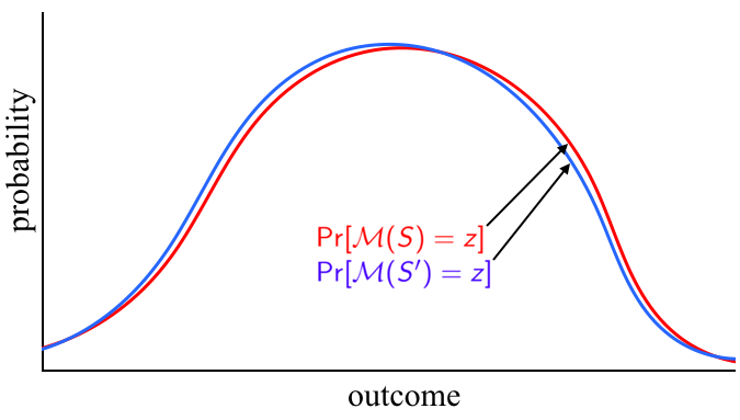
We now define the Laplace mechanism, which can be used to guarantee differential privacy.

Definition 44 (Laplace mechanism).

Given $n$ inputs in $[0,1]$ , the Laplace mechanism for outputting their average computes the true average value $a$ and then outputs $a+x$ where $x$ is drawn from the Laplace density with parameters $\left(0,\frac{1}{\alpha n}\right)$ :

\mathrm{Lap}_{(0,\frac{1}{\alpha n})}(x)=\left(\frac{\alpha n}{2}\right)e^{-|x|\alpha n}.

Theorem 45 (Dwork et al. 2006).

The Laplace mechanism satisfies $\alpha$ -differential privacy, and moreover has the property that with probability $\geq 1-\delta$ , the error added to the true average is $O\left(\frac{\log(1/\delta^{\prime})}{\alpha n}\right)$ .

It turns out the statistical queries are a perfect class of functions for applying the Laplace mechanism, which gives the result below.

Theorem 46 (Dwork et al. 2006).

If class $C$ is efficiently SQ learnable, then it is also efficiently PAC learnable while satisfying $\alpha$ -differential privacy, with time and sample size polynomial in $1/\alpha$ . In particular, if there is an algorithm that makes $M$ queries of tolerance $\tau$ to learn $C$ to error $\epsilon$ in the SQ model, then a sample of size

m=O\left(\left[\frac{M}{\alpha\tau}+\frac{M}{\tau^{2}}\right]\log\left(\frac{M}{\delta}\right)\right)

is sufficient to PAC learn $C$ to error $\epsilon$ with probability $1-\delta$ while satisfying $\alpha$ -differential privacy.

This is achieved by taking large enough sample and adding Laplace noise with scale parameter as to satisfy $\frac{\alpha}{M}$ -differential privacy per query while staying within $\tau$ of the expectation of each query.

As we have seen SQ learnability is a sufficient condition for differentially-private learnability, but it is not a necessary one. It turns out, however, that information-theoretically, SQ learnability is equivalent to a more restricted notion of privacy called local differential privacy.

Informally, local differential privacy asks not only the output of the mechanism to be differentially private but also the data itself to be differentially private with respect to the (possibly untrusted) mechanism. Hence, noise needs to be added to the data itself.

We state the connection below without providing details.

Theorem 47 (Kasiviswanathan et al. 2011).

Concept class $C$ is locally differentially privately learnable if and only if $C$ is learnable using statistical queries.⁷⁷ 7 This result is only known for the sequentially interactive model of local differential privacy. The analogous question for fully interactive differential privacy is still open. [Joseph et al. 2020]

4.3.2 Adaptive data analysis

Interestingly, differential privacy has applications to an even newer of study called adaptive data analysis, which was introduced by Dwork et al. 2015.

The main question in this area asks to what extent it is possible to answer adaptive queries accurately given a sample without assuming anything about their complexity (e.g. without limiting their VC dimension or Rademacher complexity).

Definition 48 (adaptive accuracy).

A mechanism $\mathcal{M}$ is $(\alpha,\beta)$ -accurate on a distribution $D$ and on queries $q_{1},\ldots,q_{k}$ , if for its responses $a_{1},\ldots a_{k}$ we have

\mathbf{Pr}_{\mathcal{M}}[\max|q_{i}(D)-a_{i}|\leq\alpha]\geq 1-\beta.

Note: there is also an analogous notion of $(\alpha,\beta)$ accuracy on a sample $S$ .

A natural question is how many samples from $D$ are needed to answer $k$ queries adaptively with $(\alpha,\beta)$ -accuracy. Because there is no assumption about the complexity of the class from which the $q_{i}$ s come. So, standard techniques don’t apply.

Differential privacy, however, gives us the techniques needed to answer this question by providing a notion of stability that transfers to guarantees of adaptive accuracy. The following is an example of such a transfer theorem.

Theorem 49 (Dwork et al. 2015).

Let $\mathcal{M}$ be a mechanism that on sample $S\sim D^{n}$ answers $k$ adaptively chosen statistical queries, is $\left(\frac{\alpha}{64},\frac{\alpha\beta}{32}\right)$ -private for some $\alpha,\beta>0$ and $\left(\frac{\alpha}{8},\frac{\alpha\beta}{16}\right)$ -accurate on $S$ . Then $\mathcal{M}$ is $(\alpha,\beta)$ -accurate on $D$ .

Putting together the Laplace mechanism with the transfer theorem, and doing some careful analysis to improve the bounds, one can get an adaptive algorithm for SQs.

Theorem 50 (Bassily et al. 2016).

There is a polynomial-time mechanism that is $(\alpha,\beta)$ -accurate with respect to any distribution $D$ for $k$ adaptively chosen statistical queries given

m=\tilde{O}\left(\frac{\sqrt{k}\log^{3/2}(1/\beta)}{\alpha^{2}}\right)

samples from $D$ .

There are of course various improvements to this result. For example, subsampling [Kasiviswanathan et al. 2011] can speed up the Laplace mechanism without increasing the overall sample complexity of adaptive data analysis [Fish et al. 2020].

4.4 Other applications

While this survey has focused on the preceding three application areas, statistical queries have had impact in many other fields. Here, we give a sampling of some statements of applications, leaving it to the interested reader to learn more about these results.

The first result concerns analyzing how the statistical query dimension of a concept class can separate two classes in communication complexity.

Theorem 51 (Sherstov 2008).

Let $C$ be the class of functions $\{-1,1\}^{n}\rightarrow\{-1,1\}$ computable in $\mathrm{AC}^{\mathrm{0}}$ . If

\mathrm{SQ\mbox{-}DIM}(C)\leq O\left(2^{2^{(\log n)^{\epsilon}}}\right)

for every constant $\epsilon>0$ , then

\mathrm{IP}\in\mathrm{PSPACE}^{\mathrm{cc}}\setminus\mathrm{PH}^{\mathrm{cc}}.

Another application is distributed computing. Here we state the following Theorem informally.

Theorem 52 (Chu et al. 2006).

SQ algorithms can be put into “summation form” and automatically parallelized in MapReduce, giving nearly-linear speedups in practice.

The final application we cover applies to streaming algorithms, relating the learnability of a class with statistical queries to learnability from a stream.

Theorem 53 (Steinhardt et al. 2016).

Any class $\mathcal{C}$ that is learnable with $m$ statistical queries of tolerance $1/m$ , it is learnable from a stream of $\mathrm{poly}(m,log|\mathcal{C}|)$ examples and $b=O(\log|\mathcal{C}|\log(m))$ bits of memory.

5 Discussion and some open problems

To summarize, we saw that statistical queries originate from a framework motivated, in part, for producing noise-tolerant algorithms. However, it turns out that actually most of our algorithms can be (approximately) made to work in the statistical query framework, which explains many of our impediments in learning and optimization. Statistical queries have also had applications that have shed light on the difficulty of other problems. There were also perhaps unexpected applications, to differential privacy, adaptive data analysis, evolvability, among other areas.

It is perhaps appropriate to conclude with some open questions arising from the vast literature on statistical queries, some of which this survey has not even covered. One important but difficult direction is to find new and clearly non-statistical approaches to the many problems for which statistical algorithms are known to fail due to the lower bounds presented herein.

We will not attempt to give a comprehensive or even a long list of specific open questions across the various areas; rather, we will give a sampling. Many questions are more technical – for example, the Blum et al. 2003 result separating PAC under classification noise only holds for constant noise rates – can this be generalized to noise rates approaching $1/2$ as allowed by the Angluin and Laird 1987 model? Other directions include precisely determining the sample complexity of adaptively answering SQs – the strongest known lower bound, due to [Hardt and Ullman 2014], is $\Omega(\sqrt{k}/\alpha)$ and the upper bound, due to [Bassily et al. 2016], is $O(\sqrt{k}/\alpha^{2})$ . In evolvability, we can ask about designing or analyzing faster or more natural algorithms for evolving functions (e.g. the swapping algorithm [Diochnos and Turán 2009, Valiant 2009]. In optimization, finding more problems, like planted clique, whose hardness is explained by high statistical dimension is an active area.

But the most important (and very open-ended) question may lie in thinking more broadly about where else statistical queries can have an impact. It is likely that they will find even more unexpected uses.

Acknowledgements

This survey benefitted from helpful comments by Daniel Hsu, Matthew Joseph, and Adam Klivans on its first draft. This work was supported in part by grants CCF-1934915 and CCF-1848966 from the National Science Foundation

References

Alon et al. [1998] Noga Alon, Michael Krivelevich, and Benny Sudakov. Finding a large hidden clique in a random graph. Random Struct. Algorithms, 13(3-4):457–466, 1998.
Angluin and Laird [1987] Dana Angluin and Philip D. Laird. Learning from noisy examples. Machine Learning, 2(4):343–370, 1987.
Angluin et al. [2010] Dana Angluin, David Eisenstat, Leonid Kontorovich, and Lev Reyzin. Lower bounds on learning random structures with statistical queries. In Algorithmic Learning Theory, 21st International Conference, ALT 2010, Canberra, Australia, October 6-8, 2010. Proceedings, pages 194–208, 2010.
Aslam and Decatur [1998a] Javed A. Aslam and Scott E. Decatur. Specification and simulation of statistical query algorithms for efficiency and noise tolerance. J. Comput. Syst. Sci., 56(2):191–208, 1998a.
Aslam and Decatur [1998b] Javed A. Aslam and Scott E. Decatur. General bounds on statistical query learning and PAC learning with noise via hypothesis boosting. Inf. Comput., 141(2):85–118, 1998b.
Bassily et al. [2016] Raef Bassily, Kobbi Nissim, Adam D. Smith, Thomas Steinke, Uri Stemmer, and Jonathan Ullman. Algorithmic stability for adaptive data analysis. In Proceedings of the 48th Annual ACM SIGACT Symposium on Theory of Computing, STOC 2016, Cambridge, MA, USA, June 18-21, 2016, pages 1046–1059, 2016.
Ben-David et al. [1995] Shai Ben-David, Alon Itai, and Eyal Kushilevitz. Learning by distances. Inf. Comput., 117(2):240–250, 1995.
Blum et al. [1994] Avrim Blum, Merrick L. Furst, Jeffrey C. Jackson, Michael J. Kearns, Yishay Mansour, and Steven Rudich. Weakly learning DNF and characterizing statistical query learning using fourier analysis. In Proceedings of the Twenty-Sixth Annual ACM Symposium on Theory of Computing, 23-25 May 1994, Montréal, Québec, Canada, pages 253–262, 1994.
Blum et al. [2003] Avrim Blum, Adam Kalai, and Hal Wasserman. Noise-tolerant learning, the parity problem, and the statistical query model. J. ACM, 50(4):506–519, 2003.
Blum et al. [2005] Avrim Blum, Cynthia Dwork, Frank McSherry, and Kobbi Nissim. Practical privacy: the sulq framework. In Proceedings of the Twenty-fourth ACM SIGACT-SIGMOD-SIGART Symposium on Principles of Database Systems, June 13-15, 2005, Baltimore, Maryland, USA, pages 128–138, 2005.
Bshouty and Feldman [2002] Nader H. Bshouty and Vitaly Feldman. On using extended statistical queries to avoid membership queries. Journal of Machine Learning Research, 2:359–395, 2002.
Chu et al. [2006] Cheng-Tao Chu, Sang Kyun Kim, Yi-An Lin, YuanYuan Yu, Gary R. Bradski, Andrew Y. Ng, and Kunle Olukotun. Map-reduce for machine learning on multicore. In Advances in Neural Information Processing Systems 19, Proceedings of the Twentieth Annual Conference on Neural Information Processing Systems, Vancouver, British Columbia, Canada, December 4-7, 2006, pages 281–288, 2006.
Cortes and Vapnik [1995] Corinna Cortes and Vladimir Vapnik. Support-vector networks. Mach. Learn., 20(3):273–297, 1995.
Dempster et al. [1977] A. P. Dempster, N. M. Laird, and D. B. Rubin. Maximum likelihood from incomplete data via the em algorithm. Journal of the Royal Statistical Society, Series B, 39(1):1–38, 1977.
Diochnos and Turán [2009] Dimitrios I. Diochnos and György Turán. On evolvability: The swapping algorithm, product distributions, and covariance. In Stochastic Algorithms: Foundations and Applications, 5th International Symposium, SAGA 2009, Sapporo, Japan, October 26-28, 2009. Proceedings, pages 74–88, 2009.
Dunagan and Vempala [2008] John Dunagan and Santosh Vempala. A simple polynomial-time rescaling algorithm for solving linear programs. Math. Program., 114(1):101–114, 2008.
Dwork et al. [2006] Cynthia Dwork, Frank McSherry, Kobbi Nissim, and Adam D. Smith. Calibrating noise to sensitivity in private data analysis. In Shai Halevi and Tal Rabin, editors, Theory of Cryptography, Third Theory of Cryptography Conference, TCC 2006, New York, NY, USA, March 4-7, 2006, Proceedings, volume 3876 of Lecture Notes in Computer Science, pages 265–284. Springer, 2006.
Dwork et al. [2015] Cynthia Dwork, Vitaly Feldman, Moritz Hardt, Toniann Pitassi, Omer Reingold, and Aaron Roth. The reusable holdout: Preserving validity in adaptive data analysis. Science, 349(6248):636–638, 2015. ISSN 0036-8075.
Feldman [2008] Vitaly Feldman. Evolvability from learning algorithms. In Cynthia Dwork, editor, Proceedings of the 40th Annual ACM Symposium on Theory of Computing, Victoria, British Columbia, Canada, May 17-20, 2008, pages 619–628. ACM, 2008.
Feldman [2011] Vitaly Feldman. Distribution-independent evolvability of linear threshold functions. In Sham M. Kakade and Ulrike von Luxburg, editors, COLT 2011 - The 24th Annual Conference on Learning Theory, June 9-11, 2011, Budapest, Hungary, volume 19 of JMLR Proceedings, pages 253–272. JMLR.org, 2011.
Feldman [2012] Vitaly Feldman. A complete characterization of statistical query learning with applications to evolvability. J. Comput. Syst. Sci., 78(5):1444–1459, 2012.
Feldman [2017] Vitaly Feldman. A general characterization of the statistical query complexity. In Proceedings of the 30th Conference on Learning Theory, COLT 2017, Amsterdam, The Netherlands, 7-10 July 2017, pages 785–830, 2017.
Feldman et al. [2015] Vitaly Feldman, Will Perkins, and Santosh Vempala. On the complexity of random satisfiability problems with planted solutions. In Proceedings of the Forty-Seventh Annual ACM on Symposium on Theory of Computing, STOC 2015, Portland, OR, USA, June 14-17, 2015, pages 77–86, 2015.
Feldman et al. [2017] Vitaly Feldman, Elena Grigorescu, Lev Reyzin, Santosh Srinivas Vempala, and Ying Xiao. Statistical algorithms and a lower bound for detecting planted cliques. J. ACM, 64(2):8:1–8:37, 2017.
Fish et al. [2020] Benjamin Fish, Lev Reyzin, and Benjamin I. P. Rubinstein. Sampling without compromising accuracy in adaptive data analysis. In Aryeh Kontorovich and Gergely Neu, editors, Proceedings of the 31st International Conference on Algorithmic Learning Theory, volume 117 of Proceedings of Machine Learning Research, pages 297–318, San Diego, California, USA, 08 Feb–11 Feb 2020. PMLR.
Gelfand and Smith [1990] A. E. Gelfand and A. F. M. Smith. Sampling based approaches to calculating marginal densities. Journal of the American Statistical Association, 85:398–409, 1990.
Grigorescu et al. [2011] Elena Grigorescu, Lev Reyzin, and Santosh Vempala. On noise-tolerant learning of sparse parities and related problems. In Algorithmic Learning Theory - 22nd International Conference, ALT 2011, Espoo, Finland, October 5-7, 2011. Proceedings, pages 413–424, 2011.
Hardt and Ullman [2014] Moritz Hardt and Jonathan Ullman. Preventing false discovery in interactive data analysis is hard. In 55th IEEE Annual Symposium on Foundations of Computer Science, FOCS 2014, Philadelphia, PA, USA, October 18-21, 2014, pages 454–463, 2014.
Janoos et al. [2018] Firdaus Janoos, Mehryar Mohri, and Karthik Sridharan, editors. Algorithmic Learning Theory, ALT 2018, 7-9 April 2018, Lanzarote, Canary Islands, Spain, volume 83 of Proceedings of Machine Learning Research, 2018. PMLR.
Jerrum [1992] Mark Jerrum. Large cliques elude the metropolis process. Random Struct. Algorithms, 3(4):347–360, 1992.
Joseph et al. [2020] Matthew Joseph, Jieming Mao, and Aaron Roth. Exponential separations in local differential privacy. In Shuchi Chawla, editor, Proceedings of the 2020 ACM-SIAM Symposium on Discrete Algorithms, SODA 2020, Salt Lake City, UT, USA, January 5-8, 2020, pages 515–527. SIAM, 2020.
Kanade [2011] Varun Kanade. Evolution with recombination. In IEEE 52nd Annual Symposium on Foundations of Computer Science, FOCS 2011, Palm Springs, CA, USA, October 22-25, 2011, pages 837–846, 2011.
Kasiviswanathan et al. [2011] Shiva Prasad Kasiviswanathan, Homin K. Lee, Kobbi Nissim, Sofya Raskhodnikova, and Adam D. Smith. What can we learn privately? SIAM J. Comput., 40(3):793–826, 2011.
Kearns [1998] Michael J. Kearns. Efficient noise-tolerant learning from statistical queries. J. ACM, 45(6):983–1006, 1998.
Kirkpatrick et al. [1983] S. Kirkpatrick, C. D. Gelatt, and M. P. Vecchi. Optimization by simulated annealing. Science, 220(4598):671–680, 1983. ISSN 0036-8075.
Mitra et al. [2004] Pabitra Mitra, C. A. Murthy, and Sankar K. Pal. A probabilistic active support vector learning algorithm. IEEE Trans. Pattern Anal. Mach. Intell., 26(3):413–418, 2004.
O’Donnell [2014] Ryan O’Donnell. Analysis of boolean functions. Cambridge University Press, 2014.
Pearson [1900] Karl Pearson. On the criterion that a given system of deviations from the probable in the case of a correlated system of variables is such that it can be reasonably supposed to have arisen from random sampling. The London, Edinburgh, and Dublin Philosophical Magazine and Journal of Science, 50(302):157–175, 1900.
Peikert [2014] Chris Peikert. Lattice cryptography for the internet. In Michele Mosca, editor, Post-Quantum Cryptography - 6th International Workshop, PQCrypto 2014, Waterloo, ON, Canada, October 1-3, 2014. Proceedings, volume 8772 of Lecture Notes in Computer Science, pages 197–219. Springer, 2014.
Robbins and Monro [1951] Herbert Robbins and Sutton Monro. A stochastic approximation method. Ann. Math. Statist., 22(3):400–407, 09 1951.
Schapire [1990] Robert E. Schapire. The strength of weak learnability. Machine learning, 5(2):197–227, 1990.
Sherstov [2008] Alexander A. Sherstov. Halfspace matrices. Computational Complexity, 17(2):149–178, 2008.
Sherstov [2018] Alexander A. Sherstov. Compressing interactive communication under product distributions. SIAM J. Comput., 47(2):367–419, 2018.
Simon [2007] Hans Ulrich Simon. A characterization of strong learnability in the statistical query model. In Wolfgang Thomas and Pascal Weil, editors, STACS 2007, 24th Annual Symposium on Theoretical Aspects of Computer Science, Aachen, Germany, February 22-24, 2007, Proceedings, volume 4393 of Lecture Notes in Computer Science, pages 393–404. Springer, 2007.
Steinhardt et al. [2016] Jacob Steinhardt, Gregory Valiant, and Stefan Wager. Memory, communication, and statistical queries. In Proceedings of the 29th Conference on Learning Theory, COLT 2016, New York, USA, June 23-26, 2016, pages 1490–1516, 2016.
Szörényi [2009] Balázs Szörényi. Characterizing statistical query learning: Simplified notions and proofs. In Algorithmic Learning Theory, 20th International Conference, ALT 2009, Porto, Portugal, October 3-5, 2009. Proceedings, pages 186–200, 2009.
Tanner and Wong [1987] M Tanner and W Wong. The calculation of posterior distributions by data augmentation (with discussion). Journal of the American Statistical Association, 82:528–550, 1987.
Valiant [2015] Gregory Valiant. Finding correlations in subquadratic time, with applications to learning parities and the closest pair problem. J. ACM, 62(2):13:1–13:45, 2015.
Valiant [1984] Leslie G. Valiant. A theory of the learnable. Commun. ACM, 27(11):1134–1142, 1984.
Valiant [1985] Leslie G. Valiant. Learning disjunction of conjunctions. In Aravind K. Joshi, editor, Proceedings of the 9th International Joint Conference on Artificial Intelligence. Los Angeles, CA, USA, August 1985, pages 560–566. Morgan Kaufmann, 1985.
Valiant [2009] Leslie G Valiant. Evolvability. Journal of the ACM (JACM), 56(1):3, 2009.
Vapnik and Chervonenkis [2015] Vladimir N Vapnik and A Ya Chervonenkis. On the uniform convergence of relative frequencies of events to their probabilities. In Measures of complexity, pages 11–30. Springer, 2015.
Černý [1985] V. Černý. Thermodynamical approach to the traveling salesman problem: An efficient simulation algorithm. Journal of Optimization Theory and Applications, 45(1):41–51, January 1985. ISSN 0022-3239.
Yang [2005] Ke Yang. New lower bounds for statistical query learning. J. Comput. Syst. Sci., 70(4):485–509, 2005.

$X$	$U$	$D_{010}$	$D_{011}$	$\frac{D_{010}}{U}$	$\frac{D_{011}}{U}$	$\frac{D_{010}}{U}-1$	$\frac{D_{011}}{U}-1$
000	1/8	0	0	0	0	-1	-1
001	1/8	0	1/4	0	2	-1	1
010	1/8	1/4	1/4	2	2	1	1
011	1/8	1/4	0	2	0	1	-1
100	1/8	0	0	0	0	-1	-1
101	1/8	0	1/4	0	2	-1	1
110	1/8	1/4	1/4	2	2	1	1
111	1/8	1/4	0	2	0	1	-1

$X$	$U$	$D_{010}$	$D_{011}$	$\frac{D_{010}}{U}$	$\frac{D_{011}}{U}$	$\frac{D_{010}}{U}-1$	$\frac{D_{011}}{U}-1$
000	1/8	0	0	0	0	-1	-1
001	1/8	0	1/4	0	2	-1	1
010	1/8	1/4	1/4	2	2	1	1
011	1/8	1/4	0	2	0	1	-1
100	1/8	0	0	0	0	-1	-1
101	1/8	0	1/4	0	2	-1	1
110	1/8	1/4	1/4	2	2	1	1
111	1/8	1/4	0	2	0	1	-1

Abstract

1 Introduction

2 Model, definitions, and basic results

Definition 1 (efficient PAC learning).

Definition 2 (statistical query).

Definition 3 (statistical query oracle).

Definition 4 (efficient SQ learning).

2.1 Simulating by algorithms that draw a sample

Observation 5.

Definition 6 (classification noise).

Theorem 7 (Kearns 1998).

Proof.

Theorem 8 (Aslam and Decatur 1998a).

2.2 Variants of SQs

Definition 9 (correlational statistical query oracle).

Definition 10 (honest statistical query oracle).

3 Bounds for SQ algorithms

3.1 Lower bounds

3.1.1 Statistical query dimension

Definition 11 (statistical query dimension).

Theorem 12 (Blum et al. 1994).

Proof.

Corollary 13.

Lemma 14 (Bshouty and Feldman 2002).

Proof.

Theorem 15 (Yang 2005).

3.1.2 Classes that are not efficiently SQ learnable

Observation 16.

Observation 17.

Observation 18.

Observation 19.

3.1.3 Comparison with VC dimension

Observation 20.

Proof.

Observation 21.

Proof.

Theorem 22 (Sherstov 2018).

3.2 SQ upper bounds

Observation 23.

Proof.

Theorem 24 (Aslam and Decatur 1998b).

Definition 25 (strong statistical query dimension).

3.3 The complexity of learning

4 Applications

4.1 Optimization and search over distributions

Definition 26 (The STAT, 11-STAT, and VSTAT oracles).

4.1.1 Statistical dimension

Definition 27 (pairwise correlation of two distributions).

Definition 28 (average correlation of a set of distributions).

Theorem 30 (Feldman et al. 2017).

4.1.2 Planted clique: an application of statistical dimension

Problem 31 (distributional planted kk-biclique).

Theorem 32 (Feldman et al. 2017).

Corollary 33 (Feldman et al. 2017).

4.2 Evolvability

Definition 34 (evolutionary algorithm).

Definition 35 (performance and empirical performance).

Definition 36 (selection).

Definition 37 (evolvability by an algorithm).

Definition 38 (evolvability of a concept class).

Theorem 39 (Feldman 2008).

4.2.1 Sexual evolution

Definition 40 (recombinator).

Definition 41 (parallel CSQ).

Theorem 42 (Kanade 2011).

4.3 Differential privacy and adaptive data analysis

4.3.1 Differentially private learning

Definition 43 (differential privacy).

Definition 44 (Laplace mechanism).

Theorem 45 (Dwork et al. 2006).

Theorem 46 (Dwork et al. 2006).

Theorem 47 (Kasiviswanathan et al. 2011).

4.3.2 Adaptive data analysis

Definition 48 (adaptive accuracy).

Theorem 49 (Dwork et al. 2015).

Theorem 50 (Bassily et al. 2016).

4.4 Other applications

Theorem 51 (Sherstov 2008).

Theorem 52 (Chu et al. 2006).

Theorem 53 (Steinhardt et al. 2016).

Definition 26 (The STAT, $1$ -STAT, and VSTAT oracles).

Problem 31 (distributional planted $k$ -biclique).

$X$	$U$	$D_{010}$	$D_{011}$	$\frac{D_{010}}{U}$	$\frac{D_{011}}{U}$	$\frac{D_{010}}{U}-1$	$\frac{D_{011}}{U}-1$
000	1/8	0	0	0	0	-1	-1
001	1/8	0	1/4	0	2	-1	1
010	1/8	1/4	1/4	2	2	1	1
011	1/8	1/4	0	2	0	1	-1
100	1/8	0	0	0	0	-1	-1
101	1/8	0	1/4	0	2	-1	1
110	1/8	1/4	1/4	2	2	1	1
111	1/8	1/4	0	2	0	1	-1