跳到论文正文
W Papers独立论文阅读器 arXiv:2004.00523 论文正文 计算阅读时间 · 0%
引用这篇论文根据当前论文元数据生成,正式投稿前建议核对。


License: arXiv.org perpetual non-exclusive license
arXiv:2004.00523v5 [math.AG] 17 Feb 2022

Tropical Lagrangian multi-sections and smoothing of locally free sheaves over degenerate Calabi-Yau surfaces

Kwokwai Chan Address: Department of Mathematics
The Chinese University of Hong Kong
Shatin
Hong Kong
Email address: kwchan@math.cuhk.edu.hk
, Ziming Nikolas Ma Address: Department of Mathematics
Southern University of Science and Technology
Nanshan District
Shenzhen
China
Email address: mazm@sustech.edu.cn
and Yat-Hin Suen Address: Center for Geometry and Physics
Institute for Basic Science (IBS)
Pohang 37673
Republic of Korea
Email address: yhsuen@ibs.re.kr
Date: August 11, 2026
Abstract.

We introduce the notion of tropical Lagrangian multi-sections over a 22-dimensional integral affine manifold BB with singularities, and use them to study the reconstruction problem for higher rank locally free sheaves over Calabi-Yau surfaces. To certain tropical Lagrangian multi-sections 𝕃\mathbb{L} over BB, which are explicitly constructed by prescribing local models around the ramification points, we construct locally free sheaves ℰ0​(𝕃,𝐤s)\mathcal{E}_{0}(\mathbb{L},{\bf{k}}_{s}) over the singular projective scheme X0​(B,𝒫,s)X_{0}(B,\mathscr{P},s) associated to BB equipped with a polyhedral decomposition 𝒫\mathscr{P} and a gluing data ss. We then find combinatorial conditions on such an 𝕃\mathbb{L} under which the sheaf ℰ0​(𝕃,𝐤s)\mathcal{E}_{0}(\mathbb{L},{\bf{k}}_{s}) is simple. This produces explicit examples of smoothable pairs (X0​(B,𝒫,s),ℰ0​(𝕃,𝐤s))(X_{0}(B,\mathscr{P},s),\mathcal{E}_{0}(\mathbb{L},{\bf{k}}_{s})) in dimension 2.

1. Introduction

1.1. Background

The spectacular Gross-Siebert program [16, 17, 18] is usually referred as an algebro-geometric approach to the famous Strominger-Yau-Zaslow (SYZ) conjecture [31]. It gives an algebro-geometric way to construct mirror pairs. A polarized Calabi-Yau manifold Xˇ\check{X} near a large volume limit should admit a toric degeneration pˇ:𝒳ˇ→Δ=Spec​(ℂ⁡[[t]])\check{p}:\check{\mathcal{X}}\to\Delta=\text{Spec}(\mathbb{C}[[t]]) to a singular Calabi-Yau variety Xˇ0:=pˇ−1​(0)\check{X}_{0}:=\check{p}^{-1}(0), which appears as a union of toric varieties that intersect along toric strata. By gluing the fans of these toric components, we obtain an integral affine manifold Bˇ\check{B} with singularities together with a polyhedral decomposition 𝒫ˇ\check{\mathscr{P}}. Then by choosing a strictly convex multi-valued piecewise linear function φˇ\check{\varphi} on Bˇ\check{B}, a mirror family p:𝒳→Δp:\mathcal{X}\to\Delta can be obtained by the following procedure (the fan construction):

  1. (1)

    Take the discrete Legendre transform (B,𝒫,φ)(B,\mathscr{P},\varphi) of (Bˇ,𝒫ˇ,φˇ)(\check{B},\check{\mathscr{P}},\check{\varphi}).

  2. (2)

    Let XvX_{v} be the toric variety associated to the fan Σv\Sigma_{v}, defined around a vertex v∈Bv\in B. Glue these toric varieties together along toric divisors, possibly modified with some twisted gluing data ss, to obtain a projective scheme X0​(B,𝒫,s)X_{0}(B,\mathscr{P},s).

  3. (3)

    Smooth out X0​(B,𝒫,s)X_{0}(B,\mathscr{P},s) to obtain a family p:𝒳→Δp:\mathcal{X}\to\Delta.

This is usually referred as the reconstruction problem in mirror symmetry.

The most difficult step is (3), namely, to prove that X0​(B,𝒫,s)X_{0}(B,\mathscr{P},s) is smoothable. In [16], Gross and Siebert showed that X0​(B,𝒫,s)X_{0}(B,\mathscr{P},s) carries the structure of a log scheme and it is log smooth away from a subset Z⊂X0​(B,𝒫,s)Z\subset X_{0}(B,\mathscr{P},s) of codimension at least 2. The subset ZZ should be thought of as the singular locus of an SYZ fibration (i.e. Lagrangian torus fibration) on the original side and it was the main obstacle in the reconstruction problem. Inspired by Kontsevich-Soibelman’s earlier work [23] and Fukaya’s program [11], Kontsevich and Soibelman invented the notion of scattering diagrams in the innovative work [24] and applied it to solve the reconstruction problem in dimension 2 over non-Archimedean fields. This was extensively generalized by Gross and Siebert [18], in which they solved the reconstruction problem over ℂ\mathbb{C} in any dimension. Roughly speaking, they defined a notion called structure, which consists of combinatorial (or tropical) data called slaps and walls. Applying Kontsevich-Soibelman’s scattering diagram technique, they were able to construct a remarkable explicit order-by-order smoothing of X0​(B,𝒫,s)X_{0}(B,\mathscr{P},s). Recently, in [1] and [9], it was shown that purely algebraic techniques were enough to prove the existence of smoothing and this can be applied to a more general class of varieties (called toroidal crossings varieties).

In view of Kontsevich’s homological mirror symmetry (HMS) conjecture [22], it is natural to ask if one can reconstruct coherent sheaves from combinatorial or tropical data as well, where the latter should arise as tropical limits of Lagrangian submanifolds on the mirror side. In the rank one case, this was essentially accomplished by the series of works [14, 15, 19], in which the Gross-Siebert program was extended and applied to reconstruct (generalized) theta functions, or sections of ample line bundles, on Calabi-Yau varieties, proving a strong form of Tyurin’s conjecture [34]. This paper represents an initial attempt to tackle the reconstruction problem in the higher rank case. We will restrict our attention to the dimension 2, as in [14].

1.2. Main results

Recall that the third author of this paper demonstrated in [33] that the tangent bundle Tℙ2T_{\mathbb{P}^{2}} of the complex projective plane ℙ2\mathbb{P}^{2} can be reconstructed from some tropical data on the fan of ℙ2\mathbb{P}^{2}, which he called a tropical Lagrangian multi-section. The definition there, however, is not general enough to cover more interesting cases which could arise in mirror symmetry. In Section 3, we give a more general definition of tropical Lagrangian multi-sections over a 22-dimensional integral affine manifold BB with singularities equipped with a polyhedral decomposition 𝒫\mathscr{P}.11 1 We will later assume that (B,𝒫)(B,\mathscr{P}) positive and simple, which will put constraints on the singularities; see Section 2. We expect such an object to arise as a certain kind of tropicalization of Lagrangian multi-sections in an SYZ fibration of the mirror. Roughly speaking, it is a quadruple 𝕃:=(L,π,𝒫π,φ′)\mathbb{L}:=(L,\pi,\mathscr{P}_{\pi},\varphi^{\prime}) consisting of a topological (possibly branched) covering map π:L→B\pi:L\to B, a polyhedral decomposition 𝒫π\mathscr{P}_{\pi} on LL respecting 𝒫\mathscr{P} and a multi-valued piecewise linear function φ′\varphi^{\prime} on LL. A key difference from the usual polyhedral decomposition is that we require the ramification locus S′⊂LS^{\prime}\subset L of π:L→B\pi:L\to B to be contained in the codimension 2 strata of (L,𝒫π)(L,\mathscr{P}_{\pi}). In particular, the pullback affine structure on LL is also singular along the ramification locus S′S^{\prime} (see Definition 3.6).

Remark 1.1.

Our definition of tropical Lagrangian multi-sections recovers the cone complex associated to a toric vector bundle constructed by Payne [26], at least when the cone complex is a smooth manifold.

To construct examples of tropical Lagrangian multi-sections, we need good local models. In Section 4, we describe some explicit local models of φ′\varphi^{\prime} around the ramification points. To explain these, recall that Payne [26] used an equivariant structure of Tℙ2T_{\mathbb{P}^{2}} on each affine chart to define a piecewise linear function φ2,1\varphi_{2,1} on a 2-fold covering of |Σℙ2|≅Nℝ|\Sigma_{\mathbb{P}^{2}}|\cong N_{\mathbb{R}} that takes the form

φ2,1:={−ξ1 on ​σ0+,−ξ2 on ​σ0−ξ1 on ​σ1+,ξ1−ξ2 on ​σ1−,−ξ1+ξ2 on ​σ2+,ξ2 on ​σ2−;\varphi_{2,1}:=\begin{cases}-\xi_{1}&\text{ on }\sigma_{0}^{+},\\ -\xi_{2}&\text{ on }\sigma_{0}^{-}\\ \xi_{1}&\text{ on }\sigma_{1}^{+},\\ \xi_{1}-\xi_{2}&\text{ on }\sigma_{1}^{-},\\ -\xi_{1}+\xi_{2}&\text{ on }\sigma_{2}^{+},\\ \xi_{2}&\text{ on }\sigma_{2}^{-};\end{cases}

here σi±\sigma_{i}^{\pm} are two copies of the cone σi\sigma_{i} and (ξ1,ξ2)(\xi_{1},\xi_{2}) are affine coordinates on Nℝ≅ℝ2N_{\mathbb{R}}\cong\mathbb{R}^{2}. Our local models are simply given by varying the coefficients of the function φ2,1\varphi_{2,1} as shown in Figure 1; here m,nm,n are integers with m≠nm\neq n and we call the resulting function φm,n\varphi_{m,n}. We say that a tropical Lagrangian multi-section is of class 𝒮\mathscr{S} (denoted as 𝕃∈𝒮\mathbb{L}\in\mathscr{S}) if the multi-valued piecewise linear function φ′\varphi^{\prime} is locally modeled by φm,n\varphi_{m,n} for some m,nm,n around each ramification point of π\pi; if the same m,nm,n are used at each ramification point, we obtain a special subclass called 𝒮m,n⊂𝒮\mathscr{S}_{m,n}\subset\mathscr{S}.

Refer to caption
Figure 1. The tropical Lagrangian multi-section 𝕃\mathbb{L}

In Section 5, we construct a locally free sheaf ℰ0​(𝕃,𝐤s)\mathcal{E}_{0}(\mathbb{L},{\bf{k}}_{s}) over the singular variety X0​(B,𝒫,s)X_{0}(B,\mathscr{P},s) from a tropical Lagrangian multi-section 𝕃\mathbb{L} of class 𝒮\mathscr{S}. This is already nontrivial because there are various obstructions to the gluing process. To see that, we fix a vertex v∈Bv\in B which corresponds to a maximal toric stratum XvX_{v}. The function φ′\varphi^{\prime} defines an toric line bundle on the affine chart Ui:=Spec​(ℂ⁡[Kv​(σi)∨∩M])⊂XvU_{i}:=\text{Spec}(\mathbb{C}[K_{v}(\sigma_{i})^{\vee}\cap M])\subset X_{v} for each σi∈𝒫m​a​x\sigma_{i}\in\mathscr{P}_{max} which contains vv. Taking direct sum produces a rank rr toric vector bundle over UiU_{i}. If the vertex v∈Bv\in B is not a branch point of π:L→B\pi:L\to B, these local pieces glue to give a rank rr bundle over XvX_{v} which splits. But when vv is a branch point of π\pi, there are two line bundles ℒi+,ℒi−\mathcal{L}_{i}^{+},\mathcal{L}_{i}^{-} over UiU_{i} which cannot be glued due to nontrivial monodromy around the ramification point v′∈π−1​(v)v^{\prime}\in\pi^{-1}(v). In such a case, we follow [33] (which was in turn motivated by Fukaya’s proposal for reconstructing bundles in [11]) and try to glue ℒi+⊕ℒi−\mathcal{L}_{i}^{+}\oplus\mathcal{L}_{i}^{-}’s equivariantly to obtain a set of naive transition functions:

τ10s​f:=(a0(w01)m00b0(w01)n),τ21s​f:=(b1(w12)n00a1(w12)m),τ02s​f:=(0b2(w20)na2(w20)m0).\tau^{sf}_{10}:=\begin{pmatrix}\frac{a_{0}}{(w_{0}^{1})^{m}}&0\\ 0&\frac{b_{0}}{(w_{0}^{1})^{n}}\end{pmatrix},\tau^{sf}_{21}:=\begin{pmatrix}\frac{b_{1}}{(w_{1}^{2})^{n}}&0\\ 0&\frac{a_{1}}{(w_{1}^{2})^{m}}\end{pmatrix},\tau^{sf}_{02}:=\begin{pmatrix}0&\frac{b_{2}}{(w_{2}^{0})^{n}}\\ \frac{a_{2}}{(w_{2}^{0})^{m}}&0\end{pmatrix}.

The problem is that these do not satisfy the cocycle condition. Thus we have to modify τi​js​f\tau_{ij}^{sf} by multiplication by an invertible factor Θi​j\Theta_{ij} (the wall-crossing factor), namely, τi​j:=τi​js​f​Θi​j\tau_{ij}:=\tau_{ij}^{sf}\Theta_{ij}. We then obtain the following

Proposition 1.2 (=Proposition 5.1).

If we impose the condition that ∏iai​bi=−1\prod_{i}a_{i}b_{i}=-1, then

τ02​τ21​τ10=I.\tau_{02}\tau_{21}\tau_{10}=I.

Moreover, the equivariant structure defined by (2) can be extended.

From this we obtain a rank 2 toric vector bundle Em,nE_{m,n} on ℙ2\mathbb{P}^{2}, and we denote the corresponding rank 2 bundle on the toric component Xv≅ℙ2X_{v}\cong\mathbb{P}^{2} by ℰ⁡(v′)\mathcal{E}(v^{\prime}). Taking direct sum with the r−2r-2 line bundles ℒ⁡(v(α))\mathcal{L}(v^{(\alpha)}), α=1,…,r−2\alpha=1,\dots,r-2, we obtain a rank rr bundle ℰ⁡(v)\mathcal{E}(v) on XvX_{v} even when vv is a branch point of π\pi. To glue the bundles {ℰ⁡(v)}\{\mathcal{E}(v)\} together, a key observation is that the factors Θi​j\Theta_{ij} act trivially on the boundary divisors.22 2 This is because each irreducible component of the boundary divisor is isomorphic to ℙ1\mathbb{P}^{1} and hence any bundle splits into a direct sum of two line bundles; one should not expect such a nice property for dim(B)≥3\dim(B)\geq 3. However, there is further obstruction to gluing these bundles together. This obstruction, which is given by a cohomology class o𝕃​([s])∈H2​(L,ℂ×)o_{\mathbb{L}}([s])\in H^{2}(L,\mathbb{C}^{\times}), is analogous to that in [16, Theorem 2.34] that arises from gluing of the projective scheme X0​(B,𝒫,s)X_{0}(B,\mathscr{P},s).

Theorem 1.3 (=Theorem 5.5).

If o𝕃​([s])=1o_{\mathbb{L}}([s])=1, then there exists a rank rr locally free sheaf ℰ0​(𝕃,𝐤s)\mathcal{E}_{0}(\mathbb{L},{\bf{k}}_{s}) over X0​(B,𝒫,s)X_{0}(B,\mathscr{P},s).

We can now proceed to study smoothability of the pair (X0​(B,𝒫,s),ℰ0​(𝕃,𝐤s))(X_{0}(B,\mathscr{P},s),\mathcal{E}_{0}(\mathbb{L},{\bf{k}}_{s})) (see Section 6). We will assume that the polyhedral decomposition 𝒫\mathscr{P} is positive and simple, as in [16, 17, 18], as well as elementary, meaning that every cell in 𝒫\mathscr{P} is an elementary simplex.33 3 In dimension 2, every polyhedral decomposition can actually be subdivided into elementary simplices (or equivalently, standard simplices). From the Gross-Siebert program, we already know that X0​(B,𝒫,s)X_{0}(B,\mathscr{P},s) can be smoothed out to give a formal polarized family p:𝒳→Δ:=Spec​(ℂ⁡[[t]])p:\mathcal{X}\to\Delta:=\text{Spec}(\mathbb{C}[[t]]) of Calabi-Yau surfaces. We will focus on the sheaves ℰ0​(𝕃,𝐤s)\mathcal{E}_{0}(\mathbb{L},{\bf{k}}_{s}) which correspond to the tropical Lagrangian multi-sections 𝕃∈𝒮n+1,n\mathbb{L}\in\mathscr{S}_{n+1,n} (the m≥n+2m\geq n+2 cases are actually much easier).

To prove smoothability of the pair (X0​(B,𝒫,s),ℰ0​(𝕃,𝐤s))(X_{0}(B,\mathscr{P},s),\mathcal{E}_{0}(\mathbb{L},{\bf{k}}_{s})) for 𝕃∈𝒮n+1,n\mathbb{L}\in\mathscr{S}_{n+1,n}, our strategy is to apply a result in a previous work of the first and second authors [2, Corollary 4.6], for which we need the condition that H2​(X0​(B,𝒫,s),ℰ​n​d0​(ℰ0​(𝕃,𝐤s)))=0H^{2}(X_{0}(B,\mathscr{P},s),\mathcal{E}nd_{0}(\mathcal{E}_{0}(\mathbb{L},{\bf{k}}_{s})))=0. In general, it is not easy to deal with higher cohomologies. Exploiting the fact that X0​(B,𝒫,s)X_{0}(B,\mathscr{P},s) is a Calabi-Yau surface and Serre duality, we are reduced to showing that H0​(X0​(B,𝒫,s),ℰ​n​d0​(ℰ0​(𝕃,𝐤s)))=0H^{0}(X_{0}(B,\mathscr{P},s),\mathcal{E}nd_{0}(\mathcal{E}_{0}(\mathbb{L},{\bf{k}}_{s})))=0, or equivalently, that the locally free sheaf ℰ0​(𝕃,𝐤s)\mathcal{E}_{0}(\mathbb{L},{\bf{k}}_{s}) is simple.

In the rank 22 case, we are able to find a clean and checkable combinatorial condition on the tropical Lagrangian multi-section 𝕃\mathbb{L} which is equivalent to simplicity of ℰ0​(𝕃,𝐤s)\mathcal{E}_{0}(\mathbb{L},{\bf{k}}_{s}) (see Section 6.1). In order to state our main result, we consider the embedded graph G⁡(𝒫)⊂BG(\mathscr{P})\subset B given by the union of all 1-cells in the polyhedral decomposition 𝒫\mathscr{P}, and then let

G0​(𝕃)⊂G​(𝒫)G_{0}(\mathbb{L})\subset G(\mathscr{P})

be the subgraph obtained by removing all the branch vertices and the adjacent edges. We call a 1-cycle γ⊂G0​(𝕃)\gamma\subset G_{0}(\mathbb{L}) which bounds a 2-cell in 𝒫\mathscr{P} a minimal cycle (see Definition 6.2). The key observation is that a nontrivial endomorphism of ℰ0​(𝕃,𝐤s)\mathcal{E}_{0}(\mathbb{L},{\bf{k}}_{s}) gives rise to a minimal cycle in G0​(𝕃)G_{0}(\mathbb{L}), and vice versa:

Theorem 1.4 (=Theorem 6.4).

Let 𝕃∈𝒮n+1,n\mathbb{L}\in\mathscr{S}_{n+1,n}. Then the locally free sheaf ℰ0​(𝕃,𝐤s)\mathcal{E}_{0}(\mathbb{L},{\bf{k}}_{s}) is simple if and only if G0​(𝕃)G_{0}(\mathbb{L}) has no minimal cycles.

Because of this result, we say that a tropical Lagrangian multi-section 𝕃∈𝒮n+1,n\mathbb{L}\in\mathscr{S}_{n+1,n} is simple if G0​(𝕃)G_{0}(\mathbb{L}) does not contain any minimal cycles (see Definition 6.3).

Corollary 1.5 (=Corollary 6.6).

If 𝕃∈𝒮n+1,n\mathbb{L}\in\mathscr{S}_{n+1,n} is simple, then the pair (X0​(B,𝒫,s),ℰ0​(𝕃,𝐤s))(X_{0}(B,\mathscr{P},s),\mathcal{E}_{0}(\mathbb{L},{\bf{k}}_{s})) is smoothable.

The higher rank case turns out to be much more subtle, and we can only obtain some partial results (see Section 6.2). For r≥2r\geq 2, we consider a tropical Lagrangian rr-fold multi-section 𝕃\mathbb{L} over (B,𝒫)(B,\mathscr{P}) which is totally ramified, i.e. locally modeled by the rr-fold map z↦zrz\mapsto z^{r} on ℂ\mathbb{C} around each branch point v∈Sv\in S (here S:=π⁡(S′)⊂BS:=\pi(S^{\prime})\subset B denotes the branch locus of π:L→B\pi:L\to B), and satisfies certain slope conditions (see Definition 6.10). This defines another special class of tropical Lagrangian multi-sections, which we call 𝒞\mathcal{C}. The major problem is that we do not know whether there exist toric vector bundles over the toric component XvX_{v} whose cone complexes give exactly these local models (unlike the rank 2 case where we have the bundles Em,nE_{m,n}). So we make the following:

Assumption 1.6.

For each branch point v∈Sv\in S, there exists a rank rr toric vector bundle ℰ⁡(v)\mathcal{E}(v) over XvX_{v} whose cone complex satisfies the slope conditions in Definition 6.10

The bundle ℰ⁡(v)\mathcal{E}(v) associated to v∈Sv\in S, if exists, is guaranteed to be simple. Also, an analogue of Theorem 1.3 holds, namely, the collection {ℰ⁡(v)}v∈𝒫⁡(0)\{\mathcal{E}(v)\}_{v\in\mathscr{P}(0)} can be glued to produce a locally free sheaf ℰ0​(𝕃,𝐤s)\mathcal{E}_{0}(\mathbb{L},{\bf{k}}_{s}) over X0​(B,𝒫,s)X_{0}(B,\mathscr{P},s) when the obstruction vanishes. This puts us in a situation analogous to the rank 2 case.

To understand simplicity and smoothability of ℰ0​(𝕃,𝐤s)\mathcal{E}_{0}(\mathbb{L},{\bf{k}}_{s}), we define a graph analogous to G0​(𝕃)G_{0}(\mathbb{L}); however, unlike the rank 2 case, such a graph lives in the fiber product

P⁡(𝕃):=L×BL,P(\mathbb{L}):=L\times_{B}L,

which should be viewed as a certain (fiberwise) path space of 𝕃\mathbb{L}, instead of BB. There is a natural polyhedral decomposition on P⁡(𝕃)P(\mathbb{L}), given by 𝒫~:=𝒫′×𝒫𝒫′\widetilde{\mathscr{P}}:=\mathscr{P}^{\prime}\times_{\mathscr{P}}\mathscr{P}^{\prime}. The union of all 1-cells in 𝒫~\widetilde{\mathscr{P}} gives a graph G~​(𝕃)⊂P​(𝕃)\widetilde{G}(\mathbb{L})\subset P(\mathbb{L}), and we can define the subgraph G~0​(𝕃)⊂G~​(𝕃)\widetilde{G}_{0}(\mathbb{L})\subset\widetilde{G}(\mathbb{L}) by suitable removing some edges (see Definition 6.11 for the detailed definition). We remark that, when r=2r=2, the graph G~0​(𝕃)\widetilde{G}_{0}(\mathbb{L}) can be identified with G0​(𝕃)G_{0}(\mathbb{L}) via the projection π:P⁡(𝕃)→B\pi:P(\mathbb{L})\to B. Then we have the following weakened analogue of Theorem 1.4:

Theorem 1.7 (=Theorem 6.13).

Let 𝕃∈𝒞\mathbb{L}\in\mathcal{C} such that Assumption 1.6 holds. Suppose that G~0​(𝕃)\widetilde{G}_{0}(\mathbb{L}) has no minimal cycles (1-cycle which bound a 2-cell in 𝒫~\widetilde{\mathscr{P}}), and that the line bundle ℒ⁡(v~)\mathcal{L}(\widetilde{v}) associated to any v~∈G~0​(𝕃)\widetilde{v}\in\widetilde{G}_{0}(\mathbb{L}) admits a section sv~∈H0​(Xv,ℒ⁡(v~))s_{\widetilde{v}}\in H^{0}(X_{v},\mathcal{L}(\widetilde{v})) such that sv~​(pv~)≠0s_{\widetilde{v}}(p_{\widetilde{v}})\neq 0 for some torus fixed point pv~∈Xvp_{\widetilde{v}}\in X_{v}. Then ℰ0​(𝕃,𝐤s)\mathcal{E}_{0}(\mathbb{L},{\bf{k}}_{s}) is simple and hence the pair (X0​(B,𝒫,s),ℰ0​(𝕃,𝐤s))(X_{0}(B,\mathscr{P},s),\mathcal{E}_{0}(\mathbb{L},{\bf{k}}_{s})) is smoothable.

For explicit examples of smoothable pairs (X0​(B,𝒫,s),ℰ0​(𝕃,𝐤s))(X_{0}(B,\mathscr{P},s),\mathcal{E}_{0}(\mathbb{L},{\bf{k}}_{s})) obtained using the above results, see Examples 6.8, 6.9 and 6.12.

1.3. Further perspectives

We end this introduction by two remarks.

1.3.1.

First of all, associated to the locally free sheaf ℰ0​(𝕃,𝐤s)\mathcal{E}_{0}(\mathbb{L},{\bf{k}}_{s}) is a constructible sheaf ℱ\mathcal{F} on P⁡(𝕃)=L×BLP(\mathbb{L})=L\times_{B}L defined as follows: Let πB:P⁡(𝕃)→B\pi_{B}:P(\mathbb{L})\to B be the natural projection map. We define

𝒫~:={σ1′×πσ2′∣σ1′,σ2′∈𝒫π such that π(σ1′)=π(σ2′)}.\widetilde{\mathscr{P}}:=\{\sigma_{1}^{\prime}\times_{\pi}\sigma_{2}^{\prime}\mid\sigma_{1}^{\prime},\sigma_{2}^{\prime}\in\mathscr{P}_{\pi}\text{ such that }\pi(\sigma_{1}^{\prime})=\pi(\sigma_{2}^{\prime})\}.

Let {v}∈𝒫\{v\}\in\mathscr{P} be a vertex and v~=(v1′,v2′)∈πB−1​(v)\widetilde{v}=(v_{1}^{\prime},v_{2}^{\prime})\in\pi_{B}^{-1}(v). Each vi′v_{i}^{\prime} gives a vector bundle ℰ⁡(vi′)\mathcal{E}(v_{i}^{\prime}) on XvX_{v}, which is either a line bundle or a rank 2 bundle. For σ~∈𝒫~\widetilde{\sigma}\in\widetilde{\mathscr{P}} with v~∈σ~\widetilde{v}\in\widetilde{\sigma}, we define

ℱ⁡(σ~):=H0​(Xσ,(ℰ​(v1′)∗⊗ℰ⁡(v2′))|Xσ),\mathcal{F}(\widetilde{\sigma}):=H^{0}(X_{\sigma},(\mathcal{E}(v_{1}^{\prime})^{*}\otimes\mathcal{E}(v_{2}^{\prime}))|_{X_{\sigma}}),

where σ:=πB​(σ~)\sigma:=\pi_{B}(\widetilde{\sigma}). For τ~⊂σ~\widetilde{\tau}\subset\widetilde{\sigma}, the generalization map gτ~​σ~:ℱ⁡(τ~)→ℱ⁡(σ~)g_{\widetilde{\tau}\widetilde{\sigma}}:\mathcal{F}(\widetilde{\tau})\to\mathcal{F}(\widetilde{\sigma}) is induced by the inclusion ισ​τ:Xσ↪Xτ\iota_{\sigma\tau}:X_{\sigma}\hookrightarrow X_{\tau}. Clearly, gρ~​σ~=gτ~​σ~∘gρ~​τ~g_{\widetilde{\rho}\widetilde{\sigma}}=g_{\widetilde{\tau}\widetilde{\sigma}}\circ g_{\widetilde{\rho}\widetilde{\tau}}, whenever ρ~⊂τ~⊂σ~\widetilde{\rho}\subset\widetilde{\tau}\subset\widetilde{\sigma}. Hence the data ({ℱ⁡(σ~)},{gτ~​σ~})\left(\{\mathcal{F}(\widetilde{\sigma})\},\{g_{\widetilde{\tau}\widetilde{\sigma}}\}\right) defines a constructible sheaf ℱ\mathcal{F} on P⁡(𝕃)P(\mathbb{L}) (see e.g. [20]).

Let P0​(𝕃):=P⁡(𝕃)\ΔLP_{0}(\mathbb{L}):=P(\mathbb{L})\backslash\Delta_{L}, where ΔL\Delta_{L} denotes the diagonal. By restricting ℱ\mathcal{F} to P0​(𝕃)P_{0}(\mathbb{L}), we get a sheaf ℱ0\mathcal{F}_{0} on P0​(𝕃)P_{0}(\mathbb{L}). By construction, we have canonical identifications

(1) H0​(X0​(B,𝒫,s),ℰ​n​d​(ℰ0​(𝕃,𝐤s)))≅H0​(P⁡(𝕃),ℱ),H0​(X0​(B,𝒫,s),ℰ​n​d0​(ℰ0​(𝕃,𝐤s)))≅H0​(P0​(𝕃),ℱ0).\begin{split}H^{0}(X_{0}(B,\mathscr{P},s),\mathcal{E}nd(\mathcal{E}_{0}(\mathbb{L},{\bf{k}}_{s})))&\cong H^{0}(P(\mathbb{L}),\mathcal{F}),\\ H^{0}(X_{0}(B,\mathscr{P},s),\mathcal{E}nd_{0}(\mathcal{E}_{0}(\mathbb{L},{\bf{k}}_{s})))&\cong H^{0}(P_{0}(\mathbb{L}),\mathcal{F}_{0}).\end{split}

The coherent-constructible correspondence for toric varieties was established by Fang-Liu-Treumann-Zaslow in [5, 6] and applied to prove (a version of) homological mirror symmetry (HMS) for toric varieties in [7, 8]. As mentioned above, one should think of the fiber product P⁡(𝕃)P(\mathbb{L}) as a certain fiberwise path space of 𝕃\mathbb{L}. More precisely, for a non-singular SYZ fibration p:Xˇ→Bp:\check{X}\to B and an honest Lagrangian multi-section 𝕃⊂Xˇ\mathbb{L}\subset\check{X}, one can talk about the fiberwise geodesic path space as in [23, 25], and then a point (x1′,x2′)∈P⁡(𝕃)(x_{1}^{\prime},x_{2}^{\prime})\in P(\mathbb{L}) can be regarded as the end points of an affine geodesic from 𝕃\mathbb{L} to itself. The identifications (1) suggest that if one consider higher rank sheaves ℰ\mathcal{E} on XX, the self-Hom space of ℰ\mathcal{E} should be computed by a certain (possibly derived) constructible sheaf on the “path space” P⁡(𝕃)P(\mathbb{L}). We leave this for future research.

1.3.2.

On the other hand, in order to put our results into the context of the HMS conjecture, it is best to apply the framework laid out in the very recent work [12]. According to Seidel [29, 30], a large volume limit of the mirror Xˇ\check{X} should be constructed by removing a normal crossing divisor DD which represents the Kähler class of Xˇ\check{X}, giving rise to a Weinstein manifold Yˇ\check{Y}. This produces a mirror pair X0X_{0} and Yˇ\check{Y} at the large complex structure/volume limits. The HMS conjecture for this pair is much simpler, due to the fact that the Fukaya category of Yˇ\check{Y} is quasi-equivalent to a category of sheaves with microlocal supports on its Lagrangian skeleton Λ\Lambda, as conjectured by Kontsevich. Much has been done along this direction; readers are referred to e.g. [7, 13, 12].

In [12], a Lagrangian skeleton Λ​(Φ)⊂Yˇ​(Φ)\Lambda(\Phi)\subset\check{Y}(\Phi) is constructed by gluing the local models in [7] according to a combinatorial structure Φ\Phi called fanifold, which can be extracted from (B,𝒫)(B,\mathscr{P}) (here we assume that the gluing data ss is trivial). Furthermore, they proved that there is a quasi-equivalence

DCoh​(X0)≅Fuk​(Yˇ​(Φ),∂∞Λ⁡(Φ)),\text{DCoh}(X_{0})\cong\text{Fuk}(\check{Y}(\Phi),\partial_{\infty}\Lambda(\Phi)),

where DCoh​(X0)\text{DCoh}(X_{0}) is the dg category of coherent sheaves on X0X_{0} and Fuk​(Yˇ​(Φ),∂∞Λ⁡(Φ))\text{Fuk}(\check{Y}(\Phi),\partial_{\infty}\Lambda(\Phi)) is the partially wrapped Fukaya category on (Yˇ​(Φ),∂∞Λ⁡(Φ))(\check{Y}(\Phi),\partial_{\infty}\Lambda(\Phi)). We believe that our locally free sheaf ℰ0​(𝕃,𝐤s)\mathcal{E}_{0}(\mathbb{L},{\bf{k}}_{s}), as an object in DCoh​(X0)\text{DCoh}(X_{0}), corresponds to a compact connected immersed exact Lagrangian 𝕃\mathbb{L} in Yˇ​(Φ)\check{Y}(\Phi). Moreover, it was conjectured in [12] that there should be a fibration π~:Yˇ​(Φ)→B\tilde{\pi}:\check{Y}(\Phi)\rightarrow B serving as an SYZ fibration in the large volume limit. If so, the Lagrangian 𝕃\mathbb{L} would be a Lagrangian multi-section in the fibration π~\tilde{\pi}.

The simplicity assumption in Definition 6.3 (in the rank 2 case) corresponds to the isomorphism H​F0​(𝕃,𝕃)≅ℂHF^{0}(\mathbb{L},\mathbb{L})\cong\mathbb{C} under HMS. In particular, it should be satisfied when 𝕃\mathbb{L} is connected and embedded in Yˇ\check{Y}. From [29, 30, 12], we expect that the Fukaya category Fuk​(Xˇ,D)\text{Fuk}(\check{X},D) can be obtained as a deformation of Fuk​(Yˇ,∂∞Λ⁡(Φ))\text{Fuk}(\check{Y},\partial_{\infty}\Lambda(\Phi)) by corrections coming from holomorphic disks which intersect DD. This deformation is mirror to the deformation of X0X_{0} that yields the mirror family p:𝒳→Sp:\mathcal{X}\rightarrow S. In this picture, when the Lagrangian 𝕃\mathbb{L} is connected and embedded, we believe that there are no holomorphic disks in Xˇ\check{X} bounded by 𝕃\mathbb{L}. This would imply that 𝕃\mathbb{L} deforms as an object in the category Fuk​(Xˇ,D)\text{Fuk}(\check{X},D). Therefore, the locally free sheaf ℰ0​(𝕃,𝐤s)\mathcal{E}_{0}(\mathbb{L},{\bf{k}}_{s}) should indeed be mirror to the Lagrangian multi-section 𝕃\mathbb{L}.

Acknowledgment

We are indebted to the anonymous referees for very constructive comments and suggestions, which have helped to greatly improve the exposition. The third author is grateful to Yamamoto Yuto for useful and joyful discussions. We would also like to thank Yong-Geun Oh and Cheol-Hyun Cho for their interest in this work.

The work of K. Chan was supported by grants of the Hong Kong Research Grants Council (Project No. CUHK14302617 & CUHK14303019) and direct grants from CUHK. The work of Z. N. Ma was supported by the Institute of Mathematical Sciences (IMS) and the Department of Mathematics at The Chinese University of Hong Kong. The work of Y.-H. Suen was supported by IBS-R003-D1.

2. The Gross-Siebert program

In this section, we review some machinery in the Gross-Siebert program, mainly following [16].

2.1. Affine manifolds with singularities and their polyhedral decompositions

Definition 2.1 ([16], Definition 1.15).

An integral affine manifold with singularities is a topological manifold BB together with a closed subset Γ⊂B\Gamma\subset B, which is a finite union of locally closed submanifolds of codimension at least 2, such that B0:=B\ΓB_{0}:=B\backslash\Gamma is an integral affine manifold (meaning that the transition functions are integral affine).

Let BB be an integral affine manifold with singularities and U⊂BU\subset B be an open subset. A continuous function f:U→ℝf:U\to\mathbb{R} is call integral affine if f|U∩B0:U∩B0→ℝf|_{U\cap B_{0}}:U\cap B_{0}\to\mathbb{R} is an integral affine function. The sheaf of integral affine functions on BB is denoted by 𝒜​f​f​(B,ℤ)\mathcal{A}ff(B,\mathbb{Z}).

Fix a rank nn free abelian group N≅ℤnN\cong\mathbb{Z}^{n} and let Nℝ:=N⊗ℤℝN_{\mathbb{R}}:=N\otimes_{\mathbb{Z}}\mathbb{R}.

Definition 2.2 ([16], Definition 1.21).

A polyhedral decomposition of a closed subset R⊂NℝR\subset N_{\mathbb{R}} is a locally finite covering 𝒫\mathscr{P} of RR by closed convex polytopes (called cells) with the property that

  1. (1)

    If σ∈𝒫\sigma\in\mathscr{P} and τ⊂σ\tau\subset\sigma is a face, then τ∈𝒫\tau\in\mathscr{P}.

  2. (2)

    If σ,σ′∈𝒫\sigma,\sigma^{\prime}\in\mathscr{P}, then σ∩σ′\sigma\cap\sigma^{\prime} is a common face of σ,σ′\sigma,\sigma^{\prime}.

We say 𝒫\mathscr{P} is integral if all vertices (0-dimensional cells) are contained in NN.

For a polyhedral decomposition 𝒫\mathscr{P} and a cell σ∈𝒫\sigma\in\mathscr{P}, we denote the relative interior of σ\sigma by

Int​(σ):=σ\⋃τ∈𝒫,τ⊊στ.\text{Int}(\sigma):=\sigma\Big\backslash\bigcup_{\tau\in\mathscr{P},\tau\subsetneq\sigma}\tau.
Definition 2.3 ([16], Definition 1.22).

Let BB be an integral affine manifold with singularities. A polyhedral decomposition of BB is a collection 𝒫\mathscr{P} of closed subsets of BB (called cells) covering BB which satisfies the following properties. If {v}∈𝒫\{v\}\in\mathscr{P} for some v∈Bv\in B, then v∉Γv\notin\Gamma, and there exist a polyhedral decomposition 𝒫v\mathscr{P}_{v} of a closed subset Rv⊂Tv​B≅Λv⊗ℝR_{v}\subset T_{v}B\cong\Lambda_{v}\otimes\mathbb{R}, which is the closure of an open neighborhood of 0∈Tv​B0\in T_{v}B, and a continuous map expv:Rv→B\exp_{v}:R_{v}\to B with expv⁡(0)=v\exp_{v}(0)=v satisfying the following conditions:

  1. (1)

    expv\exp_{v} is a local homeomorphism onto its image, is injective on Int​(τ)\text{Int}(\tau) for all τ∈𝒫v\tau\in\mathscr{P}_{v}, and is an integral affine map in some neighborhood of 0∈Rv0\in R_{v}.

  2. (2)

    For every top dimensional cell σ~∈𝒫v\widetilde{\sigma}\in\mathscr{P}_{v}, expv⁡(Int​(σ~))∩Γ=∅\exp_{v}(\text{Int}(\widetilde{\sigma}))\cap\Gamma=\emptyset and the restriction of expv\exp_{v} to Int​(σ~)\text{Int}(\widetilde{\sigma}) is an integral affine map. Furthermore, expv⁡(τ~)∈𝒫\exp_{v}(\widetilde{\tau})\in\mathscr{P} for all τ~∈𝒫v\widetilde{\tau}\in\mathscr{P}_{v}.

  3. (3)

    σ∈𝒫\sigma\in\mathscr{P} and v∈σv\in\sigma if and only if σ=expv⁡(σ~)\sigma=\exp_{v}(\widetilde{\sigma}) for some σ~∈𝒫v\widetilde{\sigma}\in\mathscr{P}_{v} with 0∈σ~0\in\widetilde{\sigma}.

  4. (4)

    Every σ∈𝒫\sigma\in\mathscr{P} contains a point vv with {v}∈𝒫\{v\}\in\mathscr{P}.

We say the polyhedral decomposition is toric if it satisfies the additional condition:

  1. (5)

    For each σ∈𝒫\sigma\in\mathscr{P}, there is a neighborhood Uσ⊂BU_{\sigma}\subset B of Int​(σ)\text{Int}(\sigma) and an integral affine submersion Sσ:Uσ→Nℝ′S_{\sigma}:U_{\sigma}\to N_{\mathbb{R}}^{\prime}, where N′N^{\prime} is a lattice of rank dim(B)−dim(σ){\dim(B)-\dim(\sigma)} and Sσ​(σ∩Uσ)={0}S_{\sigma}(\sigma\cap U_{\sigma})=\{0\}.

A polyhedral decomposition of BB is called integral if all vertices are integral points of BB.

The kk-dimensional strata of (B,𝒫)(B,\mathscr{P}) is defined by

B(k):=⋃τ:dim(τ)=kτ.B^{(k)}:=\bigcup_{\tau:\dim(\tau)=k}\tau.

If 𝒫\mathscr{P} is a toric polyhedral decomposition 𝒫\mathscr{P}, then for each τ∈𝒫\tau\in\mathscr{P}, one defines the fan Στ\Sigma_{\tau} as the collection of the cones

Kτ​(σ):=ℝ≥0⋅Sτ​(σ),K_{\tau}(\sigma):=\mathbb{R}_{\geq 0}\cdot S_{\tau}(\sigma),

where σ\sigma runs over all elements in 𝒫\mathscr{P} such that τ⊂σ\tau\subset\sigma and Int​(σ)∩Uτ≠∅\text{Int}(\sigma)\cap U_{\tau}\neq\emptyset. For a point y∈Int​(τ)\Γy\in\text{Int}(\tau)\backslash\Gamma, we put

𝒬τ:=𝒬τ,y:=Λy/Λτ,y,\mathcal{Q}_{\tau}:=\mathcal{Q}_{\tau,y}:=\Lambda_{y}/\Lambda_{\tau,y},

which can be identified with the lattice N′N^{\prime} in Condition (5) in Definition 2.3. These lattices define a sheaf 𝒬𝒫\mathcal{Q}_{\mathscr{P}} on BB.

Definition 2.4 ([16], Definition 1.43).

Let BB be an integral affine manifold with singularities and 𝒫\mathscr{P} a polyhedral decomposition of BB. Let U⊂BU\subset B be an open set. An integral piecewise linear function on UU is a continuous function φ\varphi so that φ\varphi is integral affine on U∩Int​(σ)U\cap\text{Int}(\sigma) for any top dimensional cell σ∈𝒫\sigma\in\mathscr{P}, and for any y∈U∩Int​(τ)y\in U\cap\text{Int}(\tau) (for some τ∈𝒫\tau\in\mathscr{P}), there exists a neighborhood VV of yy and f∈Γ⁡(V,𝒜​f​f​(B,ℤ))f\in\Gamma(V,\mathcal{A}ff(B,\mathbb{Z})) such that φ=f\varphi=f on V∩Int​(τ)V\cap\text{Int}(\tau). We denote the sheaf of integral piecewise linear functions on BB by 𝒫​ℒ𝒫​(B,ℤ)\mathcal{PL}_{\mathscr{P}}(B,\mathbb{Z}).

There is a natural inclusion 𝒜​f​f​(B,ℤ)↪𝒫​ℒ𝒫​(B,ℤ)\mathcal{A}ff(B,\mathbb{Z})\hookrightarrow\mathcal{PL}_{\mathscr{P}}(B,\mathbb{Z}), and we let ℳ​𝒫​ℒ𝒫\mathcal{MPL}_{\mathscr{P}} be the quotient:

0→𝒜​f​f​(B,ℤ)→𝒫​ℒ𝒫​(B,ℤ)→ℳ​𝒫​ℒ𝒫→0.0\to\mathcal{A}ff(B,\mathbb{Z})\to\mathcal{PL}_{\mathscr{P}}(B,\mathbb{Z})\to\mathcal{MPL}_{\mathscr{P}}\to 0.

Locally, an element φ∈Γ⁡(B,ℳ​𝒫​ℒ𝒫)\varphi\in\Gamma(B,\mathcal{MPL}_{\mathscr{P}}) is a collection of piecewise linear functions {φU}\{\varphi_{U}\} so that on each overlap U∩VU\cap V, the difference

φU|B0−φV|B0\varphi_{U}|_{B_{0}}-\varphi_{V}|_{B_{0}}

is an integral affine function on U∩V∩B0U\cap V\cap B_{0}.

Definition 2.5 ([16], Definition 1.45).

The sheaf ℳ​𝒫​ℒ𝒫\mathcal{MPL}_{\mathscr{P}} is called the sheaf of multi-valued piecewise linear functions of the pair (B,𝒫)(B,\mathscr{P}).

The sheaf ℳ​𝒫​ℒ𝒫\mathcal{MPL}_{\mathscr{P}} also fits into the following exact sequence:

0→i∗​Λ∗→𝒫​ℒ𝒫​(B,ℤ)/ℤ→ℳ​𝒫​ℒ𝒫→0,0\to i_{*}\Lambda^{*}\to\mathcal{PL}_{\mathscr{P}}(B,\mathbb{Z})/\mathbb{Z}\to\mathcal{MPL}_{\mathscr{P}}\to 0,

where Λ⊂T​B0\Lambda\subset TB_{0} is the lattice inherited from the integral structure and Λ∗⊂T∗​B0\Lambda^{*}\subset T^{*}B_{0} is the dual lattice.

Definition 2.6 ([16], Definition 1.46).

For each element φ∈H0​(B,ℳ​𝒫​ℒ𝒫)\varphi\in H^{0}(B,\mathcal{MPL}_{\mathscr{P}}), its image under the connecting map c1:H0​(B,ℳ​𝒫​ℒ𝒫)→H1​(B,i∗​Λ∗)c_{1}:H^{0}(B,\mathcal{MPL}_{\mathscr{P}})\to H^{1}(B,i_{*}\Lambda^{*}) is called the first Chern class of φ\varphi.

Definition 2.7 ([16], Definitions 1.47).

A section φ∈H0​(B,ℳ​𝒫​ℒ𝒫)\varphi\in H^{0}(B,\mathcal{MPL}_{\mathscr{P}}) is said to be (strictly) convex if for any vertex {v}∈𝒫\{v\}\in\mathscr{P}, there is a neighborhood U⊂BU\subset B of vv such that there is a (strictly) convex representative φi\varphi_{i}.

Definition 2.8 ([16], Definition 1.48).

A toric polyhedral decomposition 𝒫\mathscr{P} is said to be regular if there exists a strictly convex multi-valued piecewise linear function φ∈H0​(B,ℳ​𝒫​ℒ𝒫)\varphi\in H^{0}(B,\mathcal{MPL}_{\mathscr{P}}).

Assumption 2.9.

All polyhedral decompositions in this paper are assumed to be regular; in particular, they are integral and toric.

Given a regular polyhedral decomposition (𝒫,φ)(\mathscr{P},\varphi), one can obtain another affine manifold with singularities Bˇ\check{B} together with a regular polyhedral decomposition (𝒫ˇ,φˇ)(\check{\mathscr{P}},\check{\varphi}) by taking the dual cell of each cell in 𝒫\mathscr{P}. We will not give the precise construction here but let us mention some facts about (Bˇ,𝒫ˇ,φˇ)(\check{B},\check{\mathscr{P}},\check{\varphi}). Topologically, Bˇ\check{B} is same as BB and their singular loci coincide. However, their affine structures and monodromies around the singular loci are dual to each other. See [16], Section 1.4 for the precise construction of (Bˇ,𝒫ˇ,φˇ)(\check{B},\check{\mathscr{P}},\check{\varphi}).

Definition 2.10 (cf. [16], Propositions 1.50 & 1.51).

The triple (Bˇ,𝒫ˇ,φˇ)(\check{B},\check{\mathscr{P}},\check{\varphi}) is called the discrete Legendre transform of (B,𝒫,φ)(B,\mathscr{P},\varphi).

We will need the following notion later.

Definition 2.11.

A regular polyhedral decomposition 𝒫\mathscr{P} is called elementary if for any cell σ∈𝒫\sigma\in\mathscr{P}, the dual cell σˇ\check{\sigma} is an elementary simplex.

2.2. Toric degenerations

In [16], Gross and Siebert defined a toric degeneration (of Calabi-Yau varieties) as a flat family pˇ:𝒳ˇ→Δ=Spec​(ℂ⁡[[t]])\check{p}:\check{\mathcal{X}}\to\Delta=\text{Spec}(\mathbb{C}[[t]]) such that generic fiber of pˇ\check{p} is smooth and the central fiber Xˇ0:=pˇ−1​(0)\check{X}_{0}:=\check{p}^{-1}(0) is a union of toric varieties, intersecting along toric strata. By gluing the fan of each toric piece, they obtained an affine manifold with singularities Bˇ\check{B} together with a polyhedral decomposition 𝒫ˇ\check{\mathscr{P}}. When the family 𝒳ˇ\check{\mathcal{X}} is polarized, the resulting polyhedral decomposition is regular, so there is a strictly convex multi-valued piecewise linear function φˇ\check{\varphi} on Bˇ\check{B}, giving rise to the discrete Legendre transform (B,𝒫,φ)(B,\mathscr{P},\varphi) of (Bˇ,𝒫ˇ,φˇ)(\check{B},\check{\mathscr{P}},\check{\varphi}). The important reconstruction problem in mirror symmetry is asking whether one can construct another toric degeneration p:𝒳→Δp:\mathcal{X}\to\Delta (which acts as a mirror family) from (B,𝒫,φ)(B,\mathscr{P},\varphi).

In this section, we review the fan construction of the algebraic spaces associated to (B,𝒫)(B,\mathscr{P}) in [16]; with a good choice of gluing data, such spaces serve as the central fibers of the toric degenerations p:𝒳→Δp:\mathcal{X}\to\Delta and pˇ:𝒳ˇ→Δ\check{p}:\check{\mathcal{X}}\to\Delta.44 4 For the cone construction, please refer to [16, Section 2.1].

2.2.1. The fan construction

We first recall the category C​a​t​(𝒫)Cat(\mathscr{P}), whose objects are given by elements of 𝒫\mathscr{P}. To define morphisms, let B​a​r​(𝒫)Bar(\mathscr{P}) be the barycentric subdivision of 𝒫\mathscr{P}, and set

H​o​m​(τ,σ):={∅ if ​τ⊈σ,{i​d} if ​τ=σ.Hom(\tau,\sigma):=\begin{cases}\emptyset&\text{ if }\tau\nsubseteq\sigma,\\ \{id\}&\text{ if }\tau=\sigma.\end{cases}

For the case τ⊂σ\tau\subset\sigma, H​o​m​(τ,σ)Hom(\tau,\sigma) consists of all 1-simplices whose endpoints are the barycenters of τ\tau and σ\sigma. For e1∈H​o​m​(τ,σ),e2∈H​o​m​(σ,ω)e_{1}\in Hom(\tau,\sigma),e_{2}\in Hom(\sigma,\omega), the composition e2∘e1e_{2}\circ e_{1} is defined as the third edge of the unique 2-simplex containing e1,e2e_{1},e_{2}.

For each σ∈𝒫\sigma\in\mathscr{P}, the map Sσ:Uσ→𝒬σS_{\sigma}:U_{\sigma}\to\mathcal{Q}_{\sigma} defines a fan Σσ\Sigma_{\sigma} on 𝒬σ\mathcal{Q}_{\sigma}. Let XσX_{\sigma} be the toric variety associated to Σσ\Sigma_{\sigma}. For τ⊂σ\tau\subset\sigma, let

σ−1​Στ:={K∈Στ:K⊃Kτ​(σ)}.\sigma^{-1}\Sigma_{\tau}:=\{K\in\Sigma_{\tau}:K\supset K_{\tau}(\sigma)\}.

There is a fan projection pτ​σ:σ−1​Στ→Σσp_{\tau\sigma}:\sigma^{-1}\Sigma_{\tau}\to\Sigma_{\sigma}, given by quotienting along the direction Λσ\Lambda_{\sigma} and an inclusion jσ​τ:σ−1​Στ→Στj_{\sigma\tau}:\sigma^{-1}\Sigma_{\tau}\to\Sigma_{\tau}. There is a natural embedding ισ​τ:Xσ→X⁡(σ−1​Στ)⊂Xτ\iota_{\sigma\tau}:X_{\sigma}\to X(\sigma^{-1}\Sigma_{\tau})\subset X_{\tau} induced by the ring map

zm↦{zm if ​m∈K∨∩Kτ​(σ)⟂∩𝒬σ∗=((K+Λσ,ℝ)/λσ,ℝ)∨∩𝒬σ∗,0 otherwise,z^{m}\mapsto\begin{cases}z^{m}&\text{ if }m\in K^{\vee}\cap K_{\tau}(\sigma)^{\perp}\cap\mathcal{Q}_{\sigma}^{*}=((K+\Lambda_{\sigma,\mathbb{R}})/\lambda_{\sigma,\mathbb{R}})^{\vee}\cap\mathcal{Q}_{\sigma}^{*},\\ 0&\text{ otherwise},\end{cases}

for any K∈σ−1​ΣτK\in\sigma^{-1}\Sigma_{\tau}. For e∈H​o​m​(τ,σ)e\in Hom(\tau,\sigma), we define the functor FA:𝐂𝐚𝐭⁡(𝒫)→𝐒𝐜𝐡F_{A}:{\bf{Cat}}(\mathscr{P})\to{\bf{Sch}} by F⁡(τ):=XτF(\tau):=X_{\tau} and F⁡(e):=ισ​τF(e):=\iota_{\sigma\tau} the natural inclusion.

We can also twist the functor by certain gluing data. The barycentric subdivision B​a​r​(𝒫)Bar(\mathscr{P}) of 𝒫\mathscr{P} defines an open covering 𝒲:={Wτ}\mathcal{W}:=\{W_{\tau}\} of BB, where

Wτ:=⋃σ∈B​a​r​(𝒫)σ∩Int​(τ)≠∅Int​(σ).W_{\tau}:=\bigcup_{\begin{subarray}{c}\sigma\in Bar(\mathscr{P})\\ \sigma\cap\text{Int}(\tau)\neq\emptyset\end{subarray}}\text{Int}(\sigma).

For e∈H​o​m​(τ,σ)e\in Hom(\tau,\sigma), we define We:=Wτ∩WσW_{e}:=W_{\tau}\cap W_{\sigma}.

Definition 2.12 ([16], Definition 2.10).

Let SS be a scheme. A closed gluing data (for the fan picture) for 𝒫\mathscr{P} over SS is Cěch 1-cocycle s=(se)e∈∐τ,σ∈𝒫H​o​m​(τ,σ)s=(s_{e})_{e\in\coprod_{\tau,\sigma\in\mathscr{P}}Hom(\tau,\sigma)} of the sheaf 𝒬𝒫⊗ℤ𝔾m​(S)\mathcal{Q}_{\mathscr{P}}\otimes_{\mathbb{Z}}\mathbb{G}_{m}(S) with respect to the cover 𝒲\mathcal{W} of BB. Here, se∈Γ⁡(We,𝒬𝒫⊗ℤ𝔾m​(S))=𝒬σ⊗ℤ𝔾m​(S)s_{e}\in\Gamma(W_{e},\mathcal{Q}_{\mathscr{P}}\otimes_{\mathbb{Z}}\mathbb{G}_{m}(S))=\mathcal{Q}_{\sigma}\otimes_{\mathbb{Z}}\mathbb{G}_{m}(S) for e∈H​o​m​(τ,σ)e\in Hom(\tau,\sigma).

The torus 𝒬σ⊗ℤ𝔾m​(S)\mathcal{Q}_{\sigma}\otimes_{\mathbb{Z}}\mathbb{G}_{m}(S) acts on Xσ×SX_{\sigma}\times S, so an element se∈𝒬σ⊗ℤ𝔾m​(S)s_{e}\in\mathcal{Q}_{\sigma}\otimes_{\mathbb{Z}}\mathbb{G}_{m}(S) gives an automorphism se:Xσ×S→Xσ×Ss_{e}:X_{\sigma}\times S\to X_{\sigma}\times S. We then obtain an ss-twisted functor FS,s:ℭ​𝔞​𝔱​(𝒫)→𝔖​𝔠​𝔥SF_{S,s}:{\mathfrak{Cat}}(\mathscr{P})\to{\mathfrak{Sch}}_{S} by setting

FS,s​(τ):=Xτ×S,FS,s​(e):=(F⁡(s)×i​dS)∘se.\displaystyle F_{S,s}(\tau):=X_{\tau}\times S,\,F_{S,s}(e):=(F(s)\times id_{S})\circ s_{e}.

We define

X0​(B,𝒫,s):=lim⟶FS,s.X_{0}(B,\mathscr{P},s):=\lim_{\longrightarrow}F_{S,s}.

In [16], Gross and Siebert introduced a special set of gluing data, which they called open gluing data (for the fan picture). We will not go into details here (readers are referred to [16, Definition 2.25] for the precise definition), but it is essential for X0​(B,𝒫,s)X_{0}(B,\mathscr{P},s) to be the central fiber of some toric degeneration. Given such an open gluing data for (B,𝒫)(B,\mathscr{P}), one can associate a closed gluing data ss for the fan picture of (B,𝒫)(B,\mathscr{P}) (see [16, Proposition 2.32]). There is then an obstruction map o:H1​(𝒲,𝒬𝒫⊗ℤℂ×)→H2​(B,ℂ×)o:H^{1}(\mathcal{W},\mathcal{Q}_{\mathscr{P}}\otimes_{\mathbb{Z}}\mathbb{C}^{\times})\to H^{2}(B,\mathbb{C}^{\times}) such that when o⁡(s)=1o(s)=1, a projective scheme X0​(B,𝒫,s)X_{0}(B,\mathscr{P},s) can be constructed. Throughout this paper, we assume that all closed gluing data are induced by open gluing data for the fan picture. We also assume that A=ℂA=\mathbb{C} and S=Spec​(ℂ)S=\text{Spec}(\mathbb{C}). One of the main result in [16] is the following

Theorem 2.13 ([16], Theorem 5.2).

Suppose (B,𝒫)(B,\mathscr{P}) is positive and simple and ss satisfies the (LC) condition in [16, Proposition 4.25]. Then there exists a log structure on X0​(B,𝒫,s)X_{0}(B,\mathscr{P},s) and a morphism X0​(B,𝒫,s)†→S​p​e​c​(ℂ)†X_{0}(B,\mathscr{P},s)^{\dagger}\to Spec(\mathbb{C})^{\dagger} which is log smooth away from a subset Z⊂X0​(B,𝒫,s)Z\subset X_{0}(B,\mathscr{P},s) of codimension 2.

Remark 2.14.

When (B,𝒫)(B,\mathscr{P}) (and hence 𝑂𝑃𝐸𝑁(Bˇ,𝒫ˇ))(\check{B},\check{\mathscr{P}})) is positive and simple, X0​(B,𝒫,s)X_{0}(B,\mathscr{P},s) and Xˇ0​(Bˇ,𝒫ˇ,sˇ)\check{X}_{0}(\check{B},\check{\mathscr{P}},\check{s}) are mirror to each other as log Calabi-Yau spaces in an appropriate sense; see [16, Section 5.3] for details.

As aforementioned, the reconstruction problem in mirror symmetry is to construct a polarized toric degeneration p:𝒳→Δp:\mathcal{X}\to\Delta whose central fiber is given by X0​(B,𝒫,s)X_{0}(B,\mathscr{P},s) for some open gluing data ss over Spec​(ℂ)\text{Spec}(\mathbb{C}). This was solved by Gross and Siebert in [18] using an explicit order-by-order algorithm and a key combinatorial object called scattering diagram first introduced by Kontsevich and Soibelman in [24] (who first solved the reconstruction problem in dimension 2, but over non-Archimedean fields). When (B,𝒫)(B,\mathscr{P}) is positive and simple, Gross and Siebert proved that X0​(B,𝒫,s)X_{0}(B,\mathscr{P},s) is always smoothable by writing down an explicit toric degeneration.

In [17], Gross and Siebert studied a specific type of logarithmic deformations, called divisoral deformations. Similar to the classical deformation theory of schemes, the first order divisoral deformations of X0​(B,𝒫,s)X_{0}(B,\mathscr{P},s) are parametrized by a first cohomology group H1​(X0​(B,𝒫,s),j∗​ΘX0​(B,𝒫,s)†/ℂ†)H^{1}(X_{0}(B,\mathscr{P},s),j_{*}\Theta_{X_{0}(B,\mathscr{P},s)^{\dagger}/\mathbb{C}^{\dagger}}), while the obstructions lie in the second cohomology group H2​(X0​(B,𝒫,s),j∗​ΘX0​(B,𝒫,s)†/ℂ†)H^{2}(X_{0}(B,\mathscr{P},s),j_{*}\Theta_{X_{0}(B,\mathscr{P},s)^{\dagger}/\mathbb{C}^{\dagger}}) (see [17, Theorem 2.11]); here ΘX0​(B,𝒫,s)†/ℂ†\Theta_{X_{0}(B,\mathscr{P},s)^{\dagger}/\mathbb{C}^{\dagger}} is the sheaf of logarithmic tangent vectors of the log scheme X0​(B,𝒫,s)†X_{0}(B,\mathscr{P},s)^{\dagger} and j:X0​(B,𝒫,s)\Z↪X0​(B,𝒫,s)j:X_{0}(B,\mathscr{P},s)\backslash Z\hookrightarrow X_{0}(B,\mathscr{P},s) is the inclusion map. However, they did not prove existence of smoothings along this line of thought.

Very recently, the first two authors of this paper and Leung [1], by using gluing of local differential graded Batalin-Vilkovisky (dgBV) algebras and partly motivated by [17], developed an algebraic framework to prove existence of formal smoothings for singular Calabi-Yau varieties with prescribed local models. This covers the log smooth case studied by Friedman [10] and Kawamata-Namikawa [21] as well as the maximally degenerate case studied by Kontsevich-Soibelman [24] and Gross-Siebert [18]. More importantly, this approach provides a singular version of the classical Bogomolov-Tian-Todorov theory and bypasses the complicated scattering diagrams.

This framework was subsequently applied by Felten-Filip-Ruddat in [9] to produce smoothings of a very general class of varieties called toriodal crossing spaces.55 5 Applying results in Ruddat-Siebert [27], they were able to prove that the smoothings are actually analytic. Such an algebraic framework should be applicable in a variety of settings, e.g. it was applied to smoothing of pairs in [2]. In this paper, which can be regarded as a sequel to [2], we show how this approach can lead to an explicit, combinatorial construction of smoothable pairs in dimension 2.

3. Tropical Lagrangian multi-sections

In this section, we introduce the notion of a tropical Lagrangian multi-section when dim(B)=2\dim(B)=2.66 6 From this point on, we will always assume that dim(B)=2\dim(B)=2. These tropical objects should be viewed as limiting versions of Lagrangian multi-sections of a Lagrangian torus fibration (or SYZ fibration). In [3], the first and third authors of this paper considered the case of a semi-flat Lagrangian torus fibration X⁡(B)→BX(B)\to B, where a Lagrangian multi-section can be described by an unbranched covering map π:L→B\pi:L\to B together with a Lagrangian immersion into the symplectic manifold X⁡(B)X(B). However, in general (e.g., when BB is simply connected), the covering map π:L→B\pi:L\to B would have non-empty branch locus. We begin by describing what kind of covering maps is allowed.

Definition 3.1.

Let BB be a 2-dimensional integral affine manifold with singularities equipped with a polyhedral decomposition 𝒫\mathscr{P}. Let LL be a topological manifold. A rr-fold topological covering map π:L→B\pi:L\to B with branch locus SS is called admissible if

  1. (1)

    S⊂B(0)S\subset B^{(0)}, and

  2. (2)

    π−1​(B0\S)\pi^{-1}(B_{0}\backslash S) is an integral affine manifold such that π|π−1​(B0\S):π−1​(B0\S)→B0\S\pi|_{\pi^{-1}(B_{0}\backslash S)}:\pi^{-1}(B_{0}\backslash S)\to B_{0}\backslash S is an integral affine map.

An admissible covering map π:L→B\pi:L\to B is said to have simple branching if it satisfies the following extra condition:

  1. (3)

    For any x∈Bx\in B, there exists a neighborhood U⊂BU\subset B of xx such that the preimage π−1​(U)\pi^{-1}(U) can be written as

    U′∐∐i=1r−2Ui′U^{\prime}\amalg\coprod_{i=1}^{r-2}U_{i}^{\prime}

    for some open subsets U′,U1′,…,Ur−2′⊂LU^{\prime},U_{1}^{\prime},\dots,U_{r-2}^{\prime}\subset L so that π|U′:U′→U\pi|_{U^{\prime}}:U^{\prime}\to U is a (possibly branched) 22-fold covering map.

Given an admissible covering map π:L→B\pi:L\to B, the domain LL is naturally an integral affine manifold with singularities and the singular locus is given by S′∐π−1​(Γ)S^{\prime}\amalg\pi^{-1}(\Gamma), where S′⊂LS^{\prime}\subset L is the ramification locus of π:L→B\pi:L\to B. We need to distinguish these two singular sets combinatorially.

Definition 3.2.

Let BB be a 2-dimensional integral affine manifold with singularities equipped with a polyhedral decomposition 𝒫\mathscr{P}. Let π:L→B\pi:L\to B be an admissible covering map. A polyhedral decomposition of π:L→B\pi:L\to B is a collection 𝒫π\mathscr{P}_{\pi} of closed subsets of LL (also called cells) covering LL so that

  1. (1)

    π⁡(σ′)∈𝒫\pi(\sigma^{\prime})\in\mathscr{P} for all σ′∈𝒫π\sigma^{\prime}\in\mathscr{P}_{\pi};

  2. (2)

    for any σ∈𝒫\sigma\in\mathscr{P}, we have

    π−1(σ)=⋃σ′∈𝒫π:π⁡(σ′)=σσ′\pi^{-1}(\sigma)=\bigcup_{\sigma^{\prime}\in\mathscr{P}_{\pi}:\pi(\sigma^{\prime})=\sigma}\sigma^{\prime}

    and if we define the relative interior of σ′\sigma^{\prime} to be

    Int​(σ′):=π−1​(Int​(σ))∩σ′,\text{Int}(\sigma^{\prime}):=\pi^{-1}(\text{Int}(\sigma))\cap\sigma^{\prime},

    then π|Int​(σ′):Int​(σ′)→Int​(σ)\pi|_{\text{Int}(\sigma^{\prime})}:\text{Int}(\sigma^{\prime})\to\text{Int}(\sigma) is a homeomorphism; and

  3. (3)

    if π⁡(σ(α))=π⁡(σ(β))\pi(\sigma^{(\alpha)})=\pi(\sigma^{(\beta)}) and σ(α)∩σ(β)≠∅\sigma^{(\alpha)}\cap\sigma^{(\beta)}\neq\emptyset, then σ(α)∩σ(β)⊂S′\sigma^{(\alpha)}\cap\sigma^{(\beta)}\subset S^{\prime}.

We define

dim(σ′):=dim(σ)\dim(\sigma^{\prime}):=\dim(\sigma)

for all σ′∈𝒫π\sigma^{\prime}\in\mathcal{P}_{\pi} with π⁡(σ′)=σ∈𝒫\pi(\sigma^{\prime})=\sigma\in\mathscr{P}.

Clearly, if 𝒫π\mathscr{P}_{\pi} is a polyhedral decomposition of an admissible covering map π:L→B\pi:L\to B, then

π⁡(𝒫π):={π⁡(σ′)∣σ′∈𝒫π}=𝒫.\pi(\mathscr{P}_{\pi}):=\{\pi(\sigma^{\prime})\mid\sigma^{\prime}\in\mathscr{P}_{\pi}\}=\mathscr{P}.

We denote the kk-dimensional strata of (L,𝒫π)(L,\mathscr{P}_{\pi}) by

L(k):=⋃σ′:dim(σ′)=kσ′.L^{(k)}:=\bigcup_{\sigma^{\prime}:\dim(\sigma^{\prime})=k}\sigma^{\prime}.
Example 3.3.

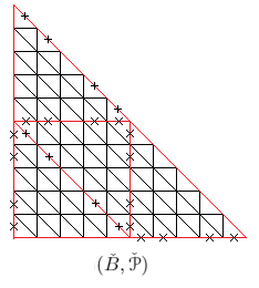
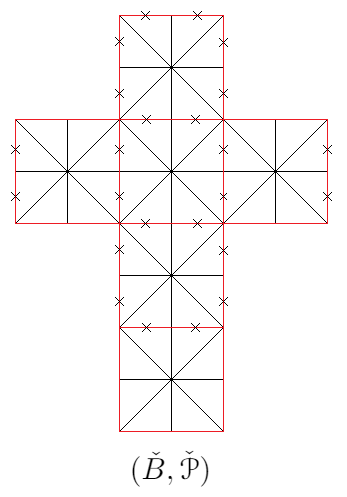
Let BB be the boundary of the unit cube in ℝ3\mathbb{R}^{3}. Let LL be a 2-torus. Then LL branches over BB at 4 points. Denote this covering map by π:L→B\pi:L\to B. We can assume the branch points (colored points) are located as in Figure 2. Vertices with same color are identified and each colored vertex on LL corresponds to a branch point on BB with the same color.

Refer to caption
Figure 2.

As the domain LL is an integral affine manifold with singularities, we can therefore define the sheaf of integral affine functions 𝒜​f​f​(L,ℤ)\mathcal{A}ff(L,\mathbb{Z}) on LL as before. However, since the singular locus S′S^{\prime} lies in L(0)L^{(0)}, we need to clarify what we mean by a piecewise linear function though it is similar to Definition 2.4:

Definition 3.4.

Let BB be an integral affine manifold with singularities equipped with a polyhedral decomposition 𝒫\mathscr{P}. Let π:L→B\pi:L\to B be an admissible covering map equipped with a polyhedral decomposition 𝒫π\mathscr{P}_{\pi}. Let U~\widetilde{U} be an open subset of LL. A piecewise linear function on U~\widetilde{U} is a continuous function φ′\varphi^{\prime} which is affine linear on Int​(σ′)\text{Int}(\sigma^{\prime}) for any maximal cell σ′∈𝒫π\sigma^{\prime}\in\mathscr{P}_{\pi} and satisfies the following property: for any y′∈U~y^{\prime}\in\widetilde{U} and y′∈Int​(τ′)y^{\prime}\in\text{Int}(\tau^{\prime}) (for some τ′∈𝒫π\tau^{\prime}\in\mathscr{P}_{\pi}), there is a neighborhood V~\widetilde{V} of y′y^{\prime} and f′∈Γ⁡(V~,𝒜​f​f​(L,ℤ))f^{\prime}\in\Gamma(\widetilde{V},\mathcal{A}ff(L,\mathbb{Z})) such that

φ′|V~∩τ′=f′|V~∩τ′.\varphi^{\prime}|_{\widetilde{V}\cap\tau^{\prime}}=f^{\prime}|_{\widetilde{V}\cap\tau^{\prime}}.

We denote the sheaf of piecewise linear functions on LL by 𝒫​ℒ𝒫π​(L,ℤ)\mathcal{PL}_{\mathscr{P}_{\pi}}(L,\mathbb{Z}).

Definition 3.5.

The sheaf of multi-valued piecewise linear functions ℳ​𝒫​ℒ𝒫π\mathcal{MPL}_{\mathscr{P}_{\pi}} on LL is defined as the quotient

0→𝒜​f​f​(L,ℤ)→𝒫​ℒ𝒫π​(L,ℤ)→ℳ​𝒫​ℒ𝒫π→0.0\to\mathcal{A}ff(L,\mathbb{Z})\to\mathcal{PL}_{\mathscr{P}_{\pi}}(L,\mathbb{Z})\to\mathcal{MPL}_{\mathscr{P}_{\pi}}\to 0.

We are now ready to define the main object to be studied in this paper.

Definition 3.6.

Let BB be a 2-dimensional integral affine manifold with singularities equipped with a polyhedral decomposition 𝒫\mathscr{P}. A tropical Lagrangian multi-section of rank rr is a quadruple 𝕃:=(L,π,𝒫π,φ′)\mathbb{L}:=(L,\pi,\mathscr{P}_{\pi},\varphi^{\prime}), where

  1. 1)

    LL is a topological manifold and π:L→B\pi:L\to B is an admissible rr-fold covering map,

  2. 2)

    𝒫π\mathscr{P}_{\pi} is a polyhedral decomposition of π:L→B\pi:L\to B, and

  3. 3)

    φ′\varphi^{\prime} is a multi-valued piecewise linear function on LL.

4. A local model around the ramification locus

In this section, we prescribe a local model for 𝕃\mathbb{L} around each ramification point of π:L→B\pi:L\to B; such a model is motivated by the work [26] of Payne and the previous work [33] of the third author. We also give an explicit construction of a certain class of rank 2 tropical Lagrangian multi-sections over BB.

Definition 4.1.

Let BB be an integral affine manifold with singularities equipped with a polyhedral decomposition 𝒫\mathscr{P}, and π:L→B\pi:L\to B an admissible covering map. A branch point v∈S⊂Bv\in S\subset B is called standard if there is an isomorphism Σv≅Σℙ2\Sigma_{v}\cong\Sigma_{\mathbb{P}^{2}} between the fan Σv\Sigma_{v} and that of ℙ2\mathbb{P}^{2}.

For a standard vertex v∈Sv\in S, we construct a fan Σv′\Sigma_{v^{\prime}}, a 22-fold covering map π∗:|Σv′|→|Σv|\pi_{*}:|\Sigma_{v^{\prime}}|\to|\Sigma_{v}| with a unique branch point at 00 and a piecewise linear function φv′:|Σv′|→ℝ\varphi_{v^{\prime}}:|\Sigma_{v^{\prime}}|\to\mathbb{R} on |Σv′||\Sigma_{v^{\prime}}| as follows.

Let Kσ0,Kσ1,Kσ2∈ΣvK_{\sigma_{0}},K_{\sigma_{1}},K_{\sigma_{2}}\in\Sigma_{v} be the top dimensional cones of Σv\Sigma_{v} which correspond to the cones σ0,σ1,σ2∈Σℙ2\sigma_{0},\sigma_{1},\sigma_{2}\in\Sigma_{\mathbb{P}^{2}} (see Figure 1) respectively. Let Kσi±K_{\sigma_{i}}^{\pm} be two copies of KσiK_{\sigma_{i}}. Let ρj,ρk\rho_{j},\rho_{k} be the rays spanning KσiK_{\sigma_{i}} and ρj±,ρk±\rho_{j}^{\pm},\rho_{k}^{\pm} be that for Kσi±K_{\sigma_{i}}^{\pm}, for i,j,k∈{0,1,2}i,j,k\in\{0,1,2\} being distinct. We glue Kσ0±K_{\sigma_{0}}^{\pm} with Kσ1∓K_{\sigma_{1}}^{\mp} and Kσ2∓K_{\sigma_{2}}^{\mp} by identifying ρ1±\rho_{1}^{\pm} with ρ1∓\rho_{1}^{\mp} and ρ2±\rho_{2}^{\pm} with ρ2∓\rho_{2}^{\mp} respectively, and glue Kσ1±K_{\sigma_{1}}^{\pm} with Kσ2∓K_{\sigma_{2}}^{\mp} by identifying ρ0±\rho_{0}^{\pm} with ρ0∓\rho_{0}^{\mp}. Then the fan Σv′\Sigma_{v^{\prime}} is given by

{Kσi±,ρi±,0∣i=0,1,2}.\{K_{\sigma_{i}}^{\pm},\rho_{i}^{\pm},0\mid i=0,1,2\}.

The projection π∗:|Σv′|→|Σv|\pi_{*}:|\Sigma_{v^{\prime}}|\to|\Sigma_{v}| is defined by Kσi±→KσiK_{\sigma_{i}}^{\pm}\to K_{\sigma_{i}}.

On the fan Σv′\Sigma_{v^{\prime}}, one can define a piecewise linear function φv′\varphi_{v^{\prime}} by setting

φv′:={(n−m)​ξ1 on ​Kσ0+,(n−m)​ξ2 on ​Kσ0−,n​ξ1 on ​Kσ1+,n​ξ1+(n−m)​ξ2 on ​Kσ1−,(n−m)​ξ1+n​ξ2 on ​Kσ2+,n​ξ2 on ​Kσ2−,\varphi_{v^{\prime}}:=\begin{cases}(n-m)\xi_{1}&\text{ on }K_{\sigma_{0}}^{+},\\ (n-m)\xi_{2}&\text{ on }K_{\sigma_{0}}^{-},\\ n\xi_{1}&\text{ on }K_{\sigma_{1}}^{+},\\ n\xi_{1}+(n-m)\xi_{2}&\text{ on }K_{\sigma_{1}}^{-},\\ (n-m)\xi_{1}+n\xi_{2}&\text{ on }K_{\sigma_{2}}^{+},\\ n\xi_{2}&\text{ on }K_{\sigma_{2}}^{-},\end{cases}

for some m,n∈ℤm,n\in\mathbb{Z} with m≠nm\neq n. Here, ξ1,ξ2\xi_{1},\xi_{2} are affine coordinates on |Σv|≅ℝ2|\Sigma_{v}|\cong\mathbb{R}^{2}. This gives a tropical Lagrangian multi-section (|Σv′|,π∗,Σv′,φv′)(|\Sigma_{v^{\prime}}|,\pi_{*},\Sigma_{v^{\prime}},\varphi_{v^{\prime}}) of the smooth affine manifold |Σv||\Sigma_{v}| with polyhedral decomposition given by the fan Σv\Sigma_{v}.

Recall that when π\pi has simple branching, for any branch point v∈Sv\in S, one can choose a neighborhood UU of vv such that

π−1​(U)=U′∐∐i=1r−2Ui′,\pi^{-1}(U)=U^{\prime}\amalg\coprod_{i=1}^{r-2}U_{i}^{\prime},

for some open subsets U′,U1′,…,Ur−2′⊂LU^{\prime},U_{1}^{\prime},\dots,U_{r-2}^{\prime}\subset L and π|U′:U′→U\pi|_{U^{\prime}}:U^{\prime}\to U is a branched 2-fold covering map. Let 𝒫π\mathscr{P}_{\pi} be a polyhedral decomposition of π:L→B\pi:L\to B. Denote by 𝒫v′\mathscr{P}_{v^{\prime}} the collection of all cells σ′∈𝒫π\sigma^{\prime}\in\mathscr{P}_{\pi} such that v′∈σ′v^{\prime}\in\sigma^{\prime}. Write

π−1​(σ∩U)∩U′=(σ+∪σ−)∩U′\pi^{-1}(\sigma\cap U)\cap U^{\prime}=(\sigma^{+}\cup\sigma^{-})\cap U^{\prime}

for σ∈𝒫\sigma\in\mathscr{P} and σ±∈𝒫v′\sigma^{\pm}\in\mathscr{P}_{v^{\prime}}.

Definition 4.2.

Let BB be a 2-dimensional integral affine manifold with singularities, 𝒫\mathscr{P} a polyhedral decomposition of BB. A tropical Lagrangian multi-section 𝕃:=(L,π,𝒫π,φ′)\mathbb{L}:=(L,\pi,\mathscr{P}_{\pi},\varphi^{\prime}) is said to be of class 𝒮\mathscr{S}, denoted as 𝕃∈𝒮\mathbb{L}\in\mathscr{S}, if

  1. (1)

    every branch point of π:L→B\pi:L\to B is standard;

  2. (2)

    for any vertex v∈Sv\in S, there exists a neighborhood U⊂BU\subset B of vv and two integral affine embeddings f′:U′→|Σv′|f^{\prime}:U^{\prime}\to|\Sigma_{v^{\prime}}|, f:U→|Σv|f:U\to|\Sigma_{v}| such that f′​(σ±∩U′)⊂Kσ±f^{\prime}(\sigma^{\pm}\cap U^{\prime})\subset K_{\sigma}^{\pm} for all σ∈𝒫\sigma\in\mathscr{P} with v∈σv\in\sigma and π∗∘f′=f∘π\pi_{*}\circ f^{\prime}=f\circ\pi; and

  3. (3)

    for each vertex v∈Sv\in S, φ′\varphi^{\prime} can be represented by φv′\varphi_{v^{\prime}} on U′U^{\prime}, i.e., if φU′′\varphi^{\prime}_{U^{\prime}} is a representative of φ′\varphi^{\prime} on U′U^{\prime}, then

    φU′′−φv′|f′​(U′)∘f′∈𝒜​f​f​(U′,ℤ),\varphi_{U^{\prime}}^{\prime}-\varphi_{v^{\prime}}|_{f^{\prime}(U^{\prime})}\circ f^{\prime}\in\mathcal{A}ff(U^{\prime},\mathbb{Z}),

    for some m⁡(v′),n⁡(v′)∈ℤm(v^{\prime}),n(v^{\prime})\in\mathbb{Z} defining φv′\varphi_{v^{\prime}}.

For fixed m,n∈ℤm,n\in\mathbb{Z} with m≠nm\neq n, there is a subclass 𝒮m,n\mathscr{S}_{m,n} of 𝒮\mathscr{S} defined as

𝒮m,n:={𝕃∈𝒮:{m⁡(v′),n⁡(v′)}={m,n}​ for all ​v′∈S′}.\mathscr{S}_{m,n}:=\{\mathbb{L}\in\mathscr{S}:\{m(v^{\prime}),n(v^{\prime})\}=\{m,n\}\text{ for all }v^{\prime}\in S^{\prime}\}.

This collection of tropical Lagrangian multi-sections will be our main object of study in Section 6.

5. Construction of ℰ0​(𝕃,𝐤s)\mathcal{E}_{0}(\mathbb{L},{\bf{k}}_{s}) for 𝕃∈𝒮\mathbb{L}\in\mathscr{S}

Let (B,𝒫)(B,\mathscr{P}) be a 2-dimensional integral affine manifold with singularities equipped with a regular polyhedral decomposition 𝒫\mathscr{P}. Let 𝕃\mathbb{L} be a rank rr tropical Lagrangian multi-section of class 𝒮\mathscr{S} as in Definition 4.2. The goal of this section is to construct a locally free sheaf ℰ0​(𝕃,𝐤s)\mathcal{E}_{0}(\mathbb{L},{\bf{k}}_{s}) of rank rr on the scheme X0​(B,𝒫,s)X_{0}(B,\mathscr{P},s) associated to 𝕃\mathbb{L} equipped with some continuous data 𝐤s{\bf{k}}_{s} which depends on the gluing data ss.

First of all, for any vertex {v}∈𝒫\{v\}\in\mathscr{P}, we need to construct a locally free sheaf ℰ⁡(v)\mathcal{E}(v) over the toric component Xv⊂X0​(B,𝒫,s)X_{v}\subset X_{0}(B,\mathscr{P},s). Let σ1,…,σl\sigma_{1},\dots,\sigma_{l} be the top dimensional cells that contain vv and Uσi⊂XvU_{\sigma_{i}}\subset X_{v} be the toric affine chart corresponding to σi\sigma_{i}. Then {Uσi}\{U_{\sigma_{i}}\} forms an open covering of XvX_{v}. Suppose the vertex v∉Sv\notin S. Then the preimage of vv consists of rr distinct points v(α)v^{(\alpha)}, for k=1,…,rk=1,\dots,r. Hence we obtain rr piecewise linear functions φv(α):|Σv(α)|→ℝ\varphi_{v^{(\alpha)}}:|\Sigma_{v^{(\alpha)}}|\to\mathbb{R}, which correspond to rr toric line bundles ℒ⁡(v(α))\mathcal{L}(v^{(\alpha)}) over XvX_{v}. The transition function of ℒ⁡(v(α))\mathcal{L}(v^{(\alpha)}) on the overlap Uv​(σ1)∩Uv​(σ2)U_{v}(\sigma_{1})\cap U_{v}(\sigma_{2}) can be chosen as

zmk​(σ1′)−mk​(σ2′),z^{m_{k}(\sigma_{1}^{\prime})-m_{k}(\sigma_{2}^{\prime})},

where mk​(σ′)m_{k}(\sigma^{\prime}) is the slope of φv(α)\varphi_{v^{(\alpha)}} on the maximal cell σ′\sigma^{\prime}. In this case, we put

ℰ⁡(v):=⨁k=1rℒ⁡(v(α)).\mathcal{E}(v):=\bigoplus_{k=1}^{r}\mathcal{L}(v^{(\alpha)}).

Now suppose v∈Sv\in S. Then by our assumption, there are precisely three top dimensional cells σ0,σ1,σ2\sigma_{0},\sigma_{1},\sigma_{2} containing vv. In this case, Xv≅ℙ2X_{v}\cong\mathbb{P}^{2}. Let v′∈S′v^{\prime}\in S^{\prime} be the unique ramification point such that π⁡(v′)=v\pi(v^{\prime})=v. In a neighborhood UU of vv, write

π−1​(σi∩U):=((σi+∪σi−)∩U′)∐∐k=1r−2σi(α)∩Uk′\pi^{-1}(\sigma_{i}\cap U):=\left((\sigma_{i}^{+}\cup\sigma_{i}^{-})\cap U^{\prime}\right)\amalg\coprod_{k=1}^{r-2}\sigma_{i}^{(\alpha)}\cap U_{k}^{\prime}

with σi+∩σi−={v′}\sigma_{i}^{+}\cap\sigma_{i}^{-}=\{v^{\prime}\} being the ramification point. As φ|U′\varphi|_{U^{\prime}} can be represented by φv′\varphi_{v^{\prime}}, by restricting to σi±,σi(α)\sigma_{i}^{\pm},\sigma_{i}^{(\alpha)}, we obtain rr integral affine functions. Hence they define rr toric line bundles ℒi±,ℒi(α)\mathcal{L}_{i}^{\pm},\mathcal{L}_{i}^{(\alpha)}, k=1,…,r−2k=1,\dots,r-2, on the affine chart Ui:=Uv​(σi)U_{i}:=U_{v}(\sigma_{i}), where

ℒ0+=\displaystyle\mathcal{L}_{0}^{+}=\, 𝒪⁡((n−m)​D1)|U0,ℒ0−=𝒪⁡((n−m)​D2)|U0,\displaystyle\mathcal{O}((n-m)D_{1})|_{U_{0}},\quad\mathcal{L}_{0}^{-}=\mathcal{O}((n-m)D_{2})|_{U_{0}},
ℒ1+=\displaystyle\mathcal{L}_{1}^{+}=\, 𝒪⁡(n​D0)|U1,ℒ1−=𝒪⁡((m−n)​D2+(2​n−m)​D0)|U1,\displaystyle\mathcal{O}(nD_{0})|_{U_{1}},\quad\quad\quad\quad\mathcal{L}_{1}^{-}=\mathcal{O}((m-n)D_{2}+(2n-m)D_{0})|_{U_{1}},
ℒ2+=\displaystyle\mathcal{L}_{2}^{+}=\, 𝒪⁡(n​D0)|U2,ℒ2−=𝒪⁡((m−n)​D1+(2​n−m)​D0)|U2.\displaystyle\mathcal{O}(nD_{0})|_{U_{2}},\quad\quad\quad\quad\mathcal{L}_{2}^{-}=\mathcal{O}((m-n)D_{1}+(2n-m)D_{0})|_{U_{2}}.

Here, Ui⊂ℙ2U_{i}\subset\mathbb{P}^{2} are the affine charts corresponding to the cones KσiK_{\sigma_{i}} and DkD_{k} is the divisor corresponding to the ray ρk\rho_{k}. In this case, we set

ℰi:=(ℒi+⊕ℒi−)⊕⨁k=1r−2ℒi(α),\mathcal{E}_{i}:=(\mathcal{L}_{i}^{+}\oplus\mathcal{L}_{i}^{-})\oplus\bigoplus_{k=1}^{r-2}\mathcal{L}_{i}^{(\alpha)},

which is a rank rr vector bundle on UσiU_{\sigma_{i}}.

Next, we try to glue the bundles ℰi\mathcal{E}_{i}’s together. First of all, the line bundles {ℒi(α)}i=0,1,2\{\mathcal{L}_{i}^{(\alpha)}\}_{i=0,1,2} naturally glue together to form a toric line bundle ℒ⁡(vk′)\mathcal{L}(v_{k}^{\prime}) on XvX_{v} as before.

However, in the case v∈Sv\in S, the rank 2 bundles {ℒi+⊕ℒi−}i=0,1,2\{\mathcal{L}_{i}^{+}\oplus\mathcal{L}_{i}^{-}\}_{i=0,1,2} cannot be glued equivariantly. This is because when we try to glue ℒi±\mathcal{L}_{i}^{\pm} to ℒj∓\mathcal{L}_{j}^{\mp} equivariantly, the gluing data consists of two diagonal matrices and one off-diagonal matrix, and so the cocycle condition fails to hold. More precisely, the equivariant structure on each ℒi+⊕ℒi−\mathcal{L}_{i}^{+}\oplus\mathcal{L}_{i}^{-} is given by the minus of the slopes of φv′\varphi_{v^{\prime}} on KσiK_{\sigma_{i}}:

(2) (λ1,λ2)⋅(w01,w02,v0+,v0−)=(λ1​w01,λ2​w02,λ1m−n​v0+,λ2m−n​v0−),(λ1,λ2)⋅(w10,w12,v1−,v1+)=(λ1−1​w10,λ1−1​λ2​w12,λ1−n​v1−,λ1−n​λ2m−n​v1+),(λ1,λ2)⋅(w20,w21,v2+,v2−)=(λ2−1​w20,λ1​λ2−1​w21,λ2−n​v2+,λ1m−n​λ2−n​v2−);\begin{split}(\lambda_{1},\lambda_{2})\cdot(w_{0}^{1},w_{0}^{2},v^{+}_{0},v^{-}_{0})&=(\lambda_{1}w_{0}^{1},\lambda_{2}w_{0}^{2},\lambda_{1}^{m-n}v^{+}_{0},\lambda_{2}^{m-n}v^{-}_{0}),\\ (\lambda_{1},\lambda_{2})\cdot(w_{1}^{0},w_{1}^{2},v^{-}_{1},v^{+}_{1})&=(\lambda_{1}^{-1}w_{1}^{0},\lambda_{1}^{-1}\lambda_{2}w_{1}^{2},\lambda_{1}^{-n}v^{-}_{1},\lambda_{1}^{-n}\lambda_{2}^{m-n}v^{+}_{1}),\\ (\lambda_{1},\lambda_{2})\cdot(w_{2}^{0},w_{2}^{1},v^{+}_{2},v^{-}_{2})&=(\lambda_{2}^{-1}w_{2}^{0},\lambda_{1}\lambda_{2}^{-1}w_{2}^{1},\lambda_{2}^{-n}v_{2}^{+},\lambda_{1}^{m-n}\lambda_{2}^{-n}v^{-}_{2});\end{split}

here vi±v_{i}^{\pm} are fiber coordinates of ℒi±\mathcal{L}_{i}^{\pm}. According to the gluing of |Σv′|\{v′}|\Sigma_{v^{\prime}}|\backslash\{v^{\prime}\}, one can write down the naive transition functions

τ10s​f:=(a0(w01)m00b0(w01)n),τ21s​f:=(b1(w12)n00a1(w12)m),τ02s​f:=(0b2(w20)na2(w20)m0),\tau^{sf}_{10}:=\begin{pmatrix}\frac{a_{0}}{(w_{0}^{1})^{m}}&0\\ 0&\frac{b_{0}}{(w_{0}^{1})^{n}}\end{pmatrix},\tau^{sf}_{21}:=\begin{pmatrix}\frac{b_{1}}{(w_{1}^{2})^{n}}&0\\ 0&\frac{a_{1}}{(w_{1}^{2})^{m}}\end{pmatrix},\tau^{sf}_{02}:=\begin{pmatrix}0&\frac{b_{2}}{(w_{2}^{0})^{n}}\\ \frac{a_{2}}{(w_{2}^{0})^{m}}&0\end{pmatrix},

where wij:=ζjζiw_{i}^{j}:=\frac{\zeta^{j}}{\zeta^{i}} are inhomogeneous coordinates of a point [ζ0:ζ1:ζ2]∈ℙ2[\zeta^{0}:\zeta^{1}:\zeta^{2}]\in\mathbb{P}^{2} and ai,bia_{i},b_{i} are arbitrary non-zero constants. It is clear that they do not compose to the identity.

To correct the gluing, we introduce three automorphisms. For m>nm>n, we consider

Θ10\displaystyle\Theta_{10} :=I+(00−a0​b1​a2​(w02w01)m−n0)∈A​u​t​(𝒪|U10⊕𝒪|U10),\displaystyle:=I+\begin{pmatrix}0&0\\ -a_{0}b_{1}a_{2}\left(\frac{w^{2}_{0}}{w^{1}_{0}}\right)^{m-n}&0\end{pmatrix}\in Aut\left(\mathcal{O}|_{U_{10}}\oplus\mathcal{O}|_{U_{10}}\right),
Θ21\displaystyle\Theta_{21} :=I+(0−a0​a1​b2​(w10w12)m−n00)∈A​u​t​(𝒪⁡(m​D0)|U21⊕𝒪⁡(n​D0)|U21),\displaystyle:=I+\begin{pmatrix}0&-a_{0}a_{1}b_{2}\left(\frac{w^{0}_{1}}{w^{2}_{1}}\right)^{m-n}\\ 0&0\end{pmatrix}\in Aut\left(\mathcal{O}(mD_{0})|_{U_{21}}\oplus\mathcal{O}(nD_{0})|_{U_{21}}\right),
Θ02\displaystyle\Theta_{02} :=I+(00−b0​a1​a2​(w21w20)m−n0)∈A​u​t​(𝒪⁡(m​D0)|U02⊕𝒪⁡(n​D0)|U02),\displaystyle:=I+\begin{pmatrix}0&0\\ -b_{0}a_{1}a_{2}\left(\frac{w^{1}_{2}}{w^{0}_{2}}\right)^{m-n}&0\end{pmatrix}\in Aut\left(\mathcal{O}(mD_{0})|_{U_{02}}\oplus\mathcal{O}(nD_{0})|_{U_{02}}\right),

while for m<nm<n, we consider

Θ10\displaystyle\Theta_{10} :=I+(0−b0​a1​b2​(w02w01)n−m00)∈A​u​t​(𝒪|U10⊕𝒪|U10),\displaystyle:=I+\begin{pmatrix}0&-b_{0}a_{1}b_{2}\left(\frac{w^{2}_{0}}{w^{1}_{0}}\right)^{n-m}\\ 0&0\end{pmatrix}\in Aut\left(\mathcal{O}|_{U_{10}}\oplus\mathcal{O}|_{U_{10}}\right),
Θ21\displaystyle\Theta_{21} :=I+(00−b0​b1​a2​(w10w12)n−m0)∈A​u​t​(𝒪⁡(m​D0)|U21⊕𝒪⁡(n​D0)|U21),\displaystyle:=I+\begin{pmatrix}0&0\\ -b_{0}b_{1}a_{2}\left(\frac{w^{0}_{1}}{w^{2}_{1}}\right)^{n-m}&0\end{pmatrix}\in Aut\left(\mathcal{O}(mD_{0})|_{U_{21}}\oplus\mathcal{O}(nD_{0})|_{U_{21}}\right),
Θ02\displaystyle\Theta_{02} :=I+(0−a0​b1​b2​(w21w20)n−m00)∈A​u​t​(𝒪⁡(m​D0)|U02⊕𝒪⁡(n​D0)|U02).\displaystyle:=I+\begin{pmatrix}0&-a_{0}b_{1}b_{2}\left(\frac{w^{1}_{2}}{w^{0}_{2}}\right)^{n-m}\\ 0&0\end{pmatrix}\in Aut\left(\mathcal{O}(mD_{0})|_{U_{02}}\oplus\mathcal{O}(nD_{0})|_{U_{02}}\right).

The factors Θi​j\Theta_{ij} are written in terms of the frame of ℰj\mathcal{E}_{j} on UjU_{j}. Let

τi​j:=τi​js​f​Θi​j.\tau_{ij}:=\tau_{ij}^{sf}\Theta_{ij}.

Then a straightforward computation gives the following

Proposition 5.1.

If we impose the condition that ∏iai​bi=−1\prod_{i}a_{i}b_{i}=-1, then

τ02​τ21​τ10=I.\tau_{02}\tau_{21}\tau_{10}=I.

Moreover, the equivariant structure defined by (2) can be extended.

Hence we obtain a rank 2 toric vector bundle Em,nE_{m,n} on Xv≅ℙ2X_{v}\cong\mathbb{P}^{2} (for v∈Sv\in S). The mysterious constants ai,bia_{i},b_{i}’s are indeed irrelevant to the holomorphic structure.

Lemma 5.2.

The holomorphic structure of Em,nE_{m,n} is independent of ai,bia_{i},b_{i}’s as long as ∏iai​bi=−1\prod_{i}a_{i}b_{i}=-1.

Proof.

We will only consider the case m>nm>n; the proof for n>mn>m is similar. Let τi​j′\tau_{ij}^{\prime}’s be the transition functions of Em,nE_{m,n} with ai=−1a_{i}=-1, bi=1b_{i}=1, for all i=0,1,2i=0,1,2. We define ff by

f|U0:=f0:=\displaystyle f|_{U_{0}}:=f_{0}:= (100a0​b1​a2),\displaystyle\begin{pmatrix}1&0\\ 0&a_{0}b_{1}a_{2}\end{pmatrix},
f|U1:=f1:=\displaystyle f|_{U_{1}}:=f_{1}:= (−a000−a1−1​b2−1),\displaystyle\begin{pmatrix}-a_{0}&0\\ 0&-a_{1}^{-1}b_{2}^{-1}\end{pmatrix},
f|U2:=f2:=\displaystyle f|_{U_{2}}:=f_{2}:= (a0​b100b2−1).\displaystyle\begin{pmatrix}a_{0}b_{1}&0\\ 0&b_{2}^{-1}\end{pmatrix}.

Using ∏iai​bi=−1\prod_{i}a_{i}b_{i}=-1, one can check that

τ02​f2=f0​τ02′,τ21​f1=f2​τ21′,τ10​f0=f1​τ10′.\tau_{02}f_{2}=f_{0}\tau_{02}^{\prime},\quad\tau_{21}f_{1}=f_{2}\tau_{21}^{\prime},\quad\tau_{10}f_{0}=f_{1}\tau_{10}^{\prime}.

Hence ff defines an isomorphism. ∎

From now on, we will take ai=−1,bi=1a_{i}=-1,b_{i}=1, for all i=0,1,2i=0,1,2. Then the corresponding transition functions are given by

(3) τ10′:=(−1(w01)m0−(w02)m−n(w01)m1(w01)n),τ21′:=(1(w12)n−(w10)m−n(w12)m0−1(w12)m),τ02′:=(−(w21)m−n(w20)m1(w20)n−1(w20)m0),\tau_{10}^{\prime}:=\begin{pmatrix}-\frac{1}{(w_{0}^{1})^{m}}&0\\ -\frac{(w_{0}^{2})^{m-n}}{(w_{0}^{1})^{m}}&\frac{1}{(w_{0}^{1})^{n}}\end{pmatrix},\tau_{21}^{\prime}:=\begin{pmatrix}\frac{1}{(w_{1}^{2})^{n}}&-\frac{(w_{1}^{0})^{m-n}}{(w_{1}^{2})^{m}}\\ 0&-\frac{1}{(w_{1}^{2})^{m}}\end{pmatrix},\tau_{02}^{\prime}:=\begin{pmatrix}-\frac{(w_{2}^{1})^{m-n}}{(w_{2}^{0})^{m}}&\frac{1}{(w_{2}^{0})^{n}}\\ -\frac{1}{(w_{2}^{0})^{m}}&0\end{pmatrix},

for m>nm>n and

τ10′:=(−1(w01)m−(w02)n−m(w01)n01(w01)n),τ21′:=(1(w12)n0−(w10)n−m(w12)n−1(w12)m),τ02′:=(01(w20)n−1(w20)m−(w21)m−n(w20)m),\tau_{10}^{\prime}:=\begin{pmatrix}-\frac{1}{(w_{0}^{1})^{m}}&-\frac{(w_{0}^{2})^{n-m}}{(w_{0}^{1})^{n}}\\ 0&\frac{1}{(w_{0}^{1})^{n}}\end{pmatrix},\tau_{21}^{\prime}:=\begin{pmatrix}\frac{1}{(w_{1}^{2})^{n}}&0\\ -\frac{(w_{1}^{0})^{n-m}}{(w_{1}^{2})^{n}}&-\frac{1}{(w_{1}^{2})^{m}}\end{pmatrix},\tau_{02}^{\prime}:=\begin{pmatrix}0&\frac{1}{(w_{2}^{0})^{n}}\\ -\frac{1}{(w_{2}^{0})^{m}}&-\frac{(w_{2}^{1})^{m-n}}{(w_{2}^{0})^{m}}\end{pmatrix},

for n>mn>m.

Proposition 5.3.

For any m,n∈ℤm,n\in\mathbb{Z} with m≠nm\neq n, we have Em,n≅En,mE_{m,n}\cong E_{n,m} and Em,n∗≅E−m,−nE_{m,n}^{*}\cong E_{-m,-n}.

Proof.

Let {τi​jm,n}\{\tau_{ij}^{m,n}\} be the transition functions of Em,nE_{m,n}. Put

J:=(0−110).J:=\begin{pmatrix}0&-1\\ 1&0\end{pmatrix}.

Then we have

τ10m,n​J=J−1​τ10n,m,τ21m,n​J−1=J​τ21n,m,τ02m,n​J=J​τ02n,m.\tau_{10}^{m,n}J=J^{-1}\tau_{10}^{n,m},\quad\tau_{21}^{m,n}J^{-1}=J\tau_{21}^{n,m},\quad\tau_{02}^{m,n}J=J\tau_{02}^{n,m}.

Hence Em,n≅En,mE_{m,n}\cong E_{n,m}. It is immediate that (τi​jm,n)−1=(τi​j−m,−n)t(\tau_{ij}^{m,n})^{-1}=(\tau_{ij}^{-m,-n})^{t}. Thus Em,n∗≅E−m,−nE_{m,n}^{*}\cong E_{-m,-n}. ∎

Before constructing the sheaf ℰ0​(𝕃,𝐤s)\mathcal{E}_{0}(\mathbb{L},{\bf{k}}_{s}), we first prove the simplicity of the rank 2 bundle Em,nE_{m,n}. This will be crucial in the study of smoothability of the pair (X0​(B,𝒫,s),ℰ0​(𝕃,𝐤s))(X_{0}(B,\mathscr{P},s),\mathcal{E}_{0}(\mathbb{L},{\bf{k}}_{s})) in Section 6. Recall that a locally free sheaf ℰ\mathcal{E} on a scheme XX is called simple if H0​(X,ℰ​n​d​(ℰ))=ℂH^{0}(X,\mathcal{E}nd(\mathcal{E}))=\mathbb{C}, or equivalently, H0​(X,ℰ​n​d0​(ℰ))=0H^{0}(X,\mathcal{E}nd_{0}(\mathcal{E}))=0 where ℰ​n​d0\mathcal{E}nd_{0} denotes the sheaf of traceless endomorphisms.

For this purpose, we compute the Chern classes of Em,nE_{m,n}. The piecewise linear function φm,n\varphi_{m,n} allows us to obtain the equivariant Chern classes as piecewise polynomial functions on |Σℙ2||\Sigma_{\mathbb{P}^{2}}| (see [26, Section 3.2]) , namely,

c1(ℂ×)2​(Em,n)=\displaystyle c_{1}^{(\mathbb{C}^{\times})^{2}}(E_{m,n})= {(n−m)​(ξ1+ξ2) on ​σ0,2​n​ξ1+(n−m)​ξ2 on ​σ1,(n−m)​ξ1+2​n​ξ2 on ​σ2.\displaystyle\begin{cases}(n-m)(\xi_{1}+\xi_{2})&\text{ on }\sigma_{0},\\ 2n\xi_{1}+(n-m)\xi_{2}&\text{ on }\sigma_{1},\\ (n-m)\xi_{1}+2n\xi_{2}&\text{ on }\sigma_{2}.\end{cases}
c2(ℂ×)2​(Em,n)=\displaystyle c_{2}^{(\mathbb{C}^{\times})^{2}}(E_{m,n})= {(n−m)2​ξ1​ξ2 on ​σ0,n2​ξ12+n⁡(n−m)​ξ1​ξ2 on ​σ1,n⁡(n−m)​ξ1​ξ2+n2​ξ22 on ​σ2.\displaystyle\begin{cases}(n-m)^{2}\xi_{1}\xi_{2}&\text{ on }\sigma_{0},\\ n^{2}\xi_{1}^{2}+n(n-m)\xi_{1}\xi_{2}&\text{ on }\sigma_{1},\\ n(n-m)\xi_{1}\xi_{2}+n^{2}\xi_{2}^{2}&\text{ on }\sigma_{2}.\end{cases}

Since the equivariant cohomology H(ℂ×)2∙​(ℙ2,ℤ)H^{\bullet}_{(\mathbb{C}^{\times})^{2}}(\mathbb{P}^{2};\mathbb{Z}) of ℙ2\mathbb{P}^{2} is given by ℤ⁡[t0,t1,t2]/(t0​t1​t2)\mathbb{Z}[t_{0},t_{1},t_{2}]/(t_{0}t_{1}t_{2}), where tit_{i}’s are piecwewise linear functions on |Σℙ2||\Sigma_{\mathbb{P}^{2}}| so that ti​(vj)=δi​jt_{i}(v_{j})=\delta_{ij}, and the forgetful map H(ℂ×)2∙​(ℙ2,ℤ)→H∙​(ℙ2,ℤ)≅ℤ⁡[H]/(H3)H^{\bullet}_{(\mathbb{C}^{\times})^{2}}(\mathbb{P}^{2};\mathbb{Z})\to H^{\bullet}(\mathbb{P}^{2};\mathbb{Z})\cong\mathbb{Z}[H]/(H^{3}) is given by mapping all the tit_{i}’s to the hyperplane class HH, we have

c⁡(Em,n)=1+(m+n)​H+(m2+n2−m​n)​H2.c(E_{m,n})=1+(m+n)H+(m^{2}+n^{2}-mn)H^{2}.
Proposition 5.4.

For all m,n∈ℤm,n\in\mathbb{Z} with m≠nm\neq n, the bundle Em,nE_{m,n} is stable and hence simple.

Proof.

A straightforward calculation shows that we have the equality

c2−4​c12=−3​(m−n)2.c_{2}-4c_{1}^{2}=-3(m-n)^{2}.

Hence c2−4​c12<0c_{2}-4c_{1}^{2}<0 and c2−4​c12≠−4c_{2}-4c_{1}^{2}\neq-4. These conditions are equivalent to stability of rank 2 bundles on ℙ2\mathbb{P}^{2}; see [28]. ∎

Let us go back to the construction of ℰ0​(𝕃,𝐤s)\mathcal{E}_{0}(\mathbb{L},{\bf{k}}_{s}). The fan structure around v∈Sv\in S defines a toric isomorphism Xv≅ℙ2X_{v}\cong\mathbb{P}^{2}. Denote the corresponding bundle on XvX_{v} by ℰ⁡(v′)\mathcal{E}(v^{\prime}) and put

ℰ⁡(v):=ℰ⁡(v′)⊕⨁k=1r−2ℒ⁡(v(α)),\mathcal{E}(v):=\mathcal{E}(v^{\prime})\oplus\bigoplus_{k=1}^{r-2}\mathcal{L}(v^{(\alpha)}),

which is a rank rr bundle on ℙ2\mathbb{P}^{2}. In this way, the tropical Lagrangian multi-section 𝕃\mathbb{L} defines a locally free sheaf ℰ⁡(σ)\mathcal{E}(\sigma) on XσX_{\sigma} for each σ∈𝒫\sigma\in\mathscr{P}. Now we fix a closed gluing data s=(se)s=(s_{e}) for the fan picture. In order to obtain a consistent gluing, we need to find a set of isomorphisms {hτ2​τ1,s:ℰ(τ2)→Fs(e)∗ℰ(τ1)}e:τ1→τ2\{h_{\tau_{2}\tau_{1},s}:\mathcal{E}(\tau_{2})\to F_{s}(e)^{*}\mathcal{E}(\tau_{1})\}_{e:\tau_{1}\to\tau_{2}} such that

(4) (Fs​(e2)∗​hτ2​τ1,s)∘hτ3​τ2,s=hτ3​τ1,s(F_{s}(e_{2})^{*}h_{\tau_{2}\tau_{1},s})\circ h_{\tau_{3}\tau_{2},s}=h_{\tau_{3}\tau_{1},s}

for e1:τ1→τ2,e2:τ2→τ3e_{1}:\tau_{1}\to\tau_{2},e_{2}:\tau_{2}\to\tau_{3} and e3:=e2∘e1e_{3}:=e_{2}\circ e_{1}.

We first construct such data for the case s=1s=1. Let e:{v}→τe:\{v\}\to\tau. If v∉Sv\notin S, then there is a natural inclusion hτ​{v}:ℰ⁡(τ)→F​(e)∗​ℰ​(v)h_{\tau\{v\}}:\mathcal{E}(\tau)\to F(e)^{*}\mathcal{E}(v), given by

hτ​{v}|Uτ​(σ):1σ(α)​(τ)↦F​(e)∗​1σ(α)​(v)h_{\tau\{v\}}|_{U_{\tau}(\sigma)}:1_{\sigma}^{(\alpha)}(\tau)\mapsto F(e)^{*}1_{\sigma}^{(\alpha)}(v)

on the affine chart Uτ​(σ)⊂XτU_{\tau}(\sigma)\subset X_{\tau}. If v∈Sv\in S, note that the transition function of ℰ⁡(v′)\mathcal{E}(v^{\prime}) on Uv​(σ1∩σ2)U_{v}(\sigma_{1}\cap\sigma_{2}) as

τσ1​σ2​(v):1v​(σ1(α))↦∑α=12ϵσ1​σ2(α​β)​zmv​(σ1(α))−mv​(σ2(β))​1v​(σ2(β)),\tau_{\sigma_{1}\sigma_{2}}(v):1_{v}(\sigma_{1}^{(\alpha)})\mapsto\sum_{\alpha=1}^{2}\epsilon_{\sigma_{1}\sigma_{2}}^{(\alpha\beta)}z^{m_{v}(\sigma_{1}^{(\alpha)})-m_{v}(\sigma_{2}^{(\beta)})}1_{v}(\sigma_{2}^{(\beta)}),

where mv​(σi(α))m_{v}(\sigma_{i}^{(\alpha)}) is the slope of the local representative of φv′\varphi_{v^{\prime}} on σi(α)\sigma_{i}^{(\alpha)} and ϵσ1​σ2(α​β)∈{0,1,−1}\epsilon_{\sigma_{1}\sigma_{2}}^{(\alpha\beta)}\in\{0,1,-1\} are prescribed as in (3). Let e:{v}→τe:\{v\}\to\tau, with τ\tau being an edge. Note that Θi​j≡I​d\Theta_{ij}\equiv Id on the divisor DkD_{k}, for i,j,k=0,1,2i,j,k=0,1,2 being distinct. The transition maps F​(e)∗​τσ1​σ2​(v)F(e)^{*}\tau_{\sigma_{1}\sigma_{2}}(v) of F​(e)∗​ℰ​(v)F(e)^{*}\mathcal{E}(v) is then given by

F​(e)∗​1v​(σ1(α))↦ϵσ1​σ2(α​α′)​(v)​zmv​(σ1(α))−mv​(σ2(α′))​F​(e)∗​1v​(σ2(α′)),F(e)^{*}1_{v}(\sigma_{1}^{(\alpha)})\mapsto\epsilon_{\sigma_{1}\sigma_{2}}^{(\alpha\alpha^{\prime})}(v)z^{m_{v}(\sigma_{1}^{(\alpha)})-m_{v}(\sigma_{2}^{(\alpha^{\prime})})}F(e)^{*}1_{v}(\sigma_{2}^{(\alpha^{\prime})}),

where α′\alpha^{\prime} is uniquely determined by the conditions v′∉σ1(α)∩σ2(α′)v^{\prime}\notin\sigma_{1}^{(\alpha)}\cap\sigma_{2}^{(\alpha^{\prime})} and π⁡(σ2(α′))=σ2\pi(\sigma_{2}^{(\alpha^{\prime})})=\sigma_{2}. Note that ϵσ1​σ2(α​α′)​(v)≠0\epsilon_{\sigma_{1}\sigma_{2}}^{(\alpha\alpha^{\prime})}(v)\neq 0 for all α\alpha. Since XτX_{\tau} is covered by two charts Uτ​(σ1),Uτ​(σ2)U_{\tau}(\sigma_{1}),U_{\tau}(\sigma_{2}), we can define

H⁡(e):{1τ​(σ1(α))↦F​(e)∗​1v​(σ1(α)) on ​Uτ​(σ1),1τ​(σ2(α))↦ϵσ1​σ2(α​α′)​(v)​F​(e)∗​1v​(σ2(α′)) on ​Uτ​(σ2).H(e):\begin{cases}1_{\tau}(\sigma_{1}^{(\alpha)})\mapsto F(e)^{*}1_{v}(\sigma_{1}^{(\alpha)})&\text{ on }U_{\tau}(\sigma_{1}),\\ 1_{\tau}(\sigma_{2}^{(\alpha)})\mapsto\epsilon_{\sigma_{1}\sigma_{2}}^{(\alpha\alpha^{\prime})}(v)F(e)^{*}1_{v}(\sigma_{2}^{(\alpha^{\prime})})&\text{ on }U_{\tau}(\sigma_{2}).\end{cases}

Then it is easy to see that

Hs​(e)|Uτ​(σ2)∘τσ1​σ2​(τ)=F​(e)∗​τσ1​σ2​(v)∘Hs​(e)|Uτ​(σ1).H_{s}(e)|_{U_{\tau}(\sigma_{2})}\circ\tau_{\sigma_{1}\sigma_{2}}(\tau)=F(e)^{*}\tau_{\sigma_{1}\sigma_{2}}(v)\circ H_{s}(e)|_{U_{\tau}(\sigma_{1})}.

Hence H⁡(e):ℰ⁡(τ)→F​(e)∗​ℰ​(v)H(e):\mathcal{E}(\tau)\to F(e)^{*}\mathcal{E}(v) defines an isomorphism. For e3:{v}→e1τ→e2σe_{3}:\{v\}\xrightarrow{e_{1}}\tau\xrightarrow{e_{2}}\sigma, with σ∈𝒫⁡(2)\sigma\in\mathscr{P}(2), we put

H⁡(e2):\displaystyle H(e_{2}):  1σ​(σ(α))↦(ϵσ1​σ2(α​α′)​(v))−1​F​(e2)∗​1τ​(σ(α)),\displaystyle\,1_{\sigma}(\sigma^{(\alpha)})\mapsto(\epsilon_{\sigma_{1}\sigma_{2}}^{(\alpha\alpha^{\prime})}(v))^{-1}F(e_{2})^{*}1_{\tau}(\sigma^{(\alpha)}),
H⁡(e3):\displaystyle H(e_{3}):  1σ​(σ(α))↦F​(e3)∗​1v​(σ(α′)).\displaystyle\,1_{\sigma}(\sigma^{(\alpha)})\mapsto F(e_{3})^{*}1_{v}(\sigma^{(\alpha^{\prime})}).

Note that H⁡(e2)H(e_{2}) is well-defined because σ1,σ2\sigma_{1},\sigma_{2} are uniquely determined by τ\tau and ϵσ1​σ2(α​α′)​(v)≠0\epsilon_{\sigma_{1}\sigma_{2}}^{(\alpha\alpha^{\prime})}(v)\neq 0. It is clear that

(5) H⁡(e3)=H⁡(e1)∘H⁡(e2).H(e_{3})=H(e_{1})\circ H(e_{2}).

Now we turn on the gluing data ss. Since all bundles that we constructed are equivariant with respective to the torus of the corresponding toric strata, there is an isomorphism ℰ⁡(τ2)≅se∗​ℰ​(τ2)\mathcal{E}(\tau_{2})\cong s_{e}^{*}\mathcal{E}(\tau_{2}), for any e:τ1→τ2e:\tau_{1}\to\tau_{2}. Therefore, we can compose hτ2​τ1h_{\tau_{2}\tau_{1}} with this isomorphism to get hτ2​τ1,sh_{\tau_{2}\tau_{1},s}. But the cocycle condition (4) may not be satisfied due to the non-trivial gluing data ss. Explicitly, by using (5), the composition

hτ3​τ1,s−1∘(Fs​(e2)∗​hτ2​τ1,s)∘hτ3​τ2,sh_{\tau_{3}\tau_{1},s}^{-1}\circ(F_{s}(e_{2})^{*}h_{\tau_{2}\tau_{1},s})\circ h_{\tau_{3}\tau_{2},s}

is given by

1σ(α)​(τ3)↦sτ1​τ2​τ3​(σ(α))−1​1σ(α)​(τ3),1_{\sigma}^{(\alpha)}(\tau_{3})\mapsto s_{\tau_{1}\tau_{2}\tau_{3}}(\sigma^{(\alpha)})^{-1}1_{\sigma}^{(\alpha)}(\tau_{3}),

where

sτ1​τ2​τ3​(σ(α)):=se2​(mτ3​(σ(α)))​se1​(mτ2​(σ(α)))​se3​(mτ3​(σ(α)))−1.s_{\tau_{1}\tau_{2}\tau_{3}}(\sigma^{(\alpha)}):=s_{e_{2}}(m_{\tau_{3}}(\sigma^{(\alpha)}))s_{e_{1}}(m_{\tau_{2}}(\sigma^{(\alpha)}))s_{e_{3}}(m_{\tau_{3}}(\sigma^{(\alpha)}))^{-1}.

Here e1:τ1→τ2,e2:τ2→τ3,e3=e2∘e1e_{1}:\tau_{1}\to\tau_{2},e_{2}:\tau_{2}\to\tau_{3},e_{3}=e_{2}\circ e_{1} and mτi​(σ(α))m_{\tau_{i}}(\sigma^{(\alpha)}) is the slope of φτi′\varphi_{\tau_{i}^{\prime}} on the cone Sτi′​(σ(α))∈Στi′S_{\tau_{i}^{\prime}}(\sigma^{(\alpha)})\in\Sigma_{\tau_{i}^{\prime}}. As Fs​(e3)=Fs​(e1)∘Fs​(e2)F_{s}(e_{3})=F_{s}(e_{1})\circ F_{s}(e_{2}), we have

sτ1​τ2​τ3​(σ1(α))=sτ1​τ2​τ3​(σ2(β)).s_{\tau_{1}\tau_{2}\tau_{3}}(\sigma_{1}^{(\alpha)})=s_{\tau_{1}\tau_{2}\tau_{3}}(\sigma_{2}^{(\beta)}).

Hence the quantity

sτ1′​τ2′​τ3′:=sτ1​τ2​τ3​(σ(α))s_{\tau_{1}^{\prime}\tau_{2}^{\prime}\tau_{3}^{\prime}}:=s_{\tau_{1}\tau_{2}\tau_{3}}(\sigma^{(\alpha)})

only depends on the lifts τ1′⊂τ2′⊂τ3′\tau_{1}^{\prime}\subset\tau_{2}^{\prime}\subset\tau_{3}^{\prime} that σ′\sigma^{\prime} contains. Also, if we choose other local representatives of φ′\varphi^{\prime}, then

s^τ1′​τ2′​τ3′=sτ1′​τ2′​τ3′​(se1​(a⁡(τ3′))​se2​(a⁡(τ2′))​se3​(a⁡(τ3′))−1),\hat{s}_{\tau_{1}^{\prime}\tau_{2}^{\prime}\tau_{3}^{\prime}}=s_{\tau_{1}^{\prime}\tau_{2}^{\prime}\tau_{3}^{\prime}}\left(s_{e_{1}}(a(\tau_{3}^{\prime}))s_{e_{2}}(a(\tau_{2}^{\prime}))s_{e_{3}}(a(\tau_{3}^{\prime}))^{-1}\right),

where a(∙′)a(\bullet^{\prime}) is the slope some affine function. Hence, for any τ1′⊂τ2′⊂τ3′\tau_{1}^{\prime}\subset\tau_{2}^{\prime}\subset\tau_{3}^{\prime}, we obtain an element sτ1′​τ2′​τ3′∈ℂ×s_{\tau_{1}^{\prime}\tau_{2}^{\prime}\tau_{3}^{\prime}}\in\mathbb{C}^{\times}, so that (sτ1′​τ2′​τ3′)τ1′⊂τ2′⊂τ3′(s_{\tau_{1}^{\prime}\tau_{2}^{\prime}\tau_{3}^{\prime}})_{\tau_{1}^{\prime}\subset\tau_{2}^{\prime}\subset\tau_{3}^{\prime}} gives a ℂ×\mathbb{C}^{\times}-valued Cěch 2-cocycle with respect to the simplicial structure on LL induced by 𝒫π\mathscr{P}_{\pi}. This defines a cohomology class

o𝕃​(s):=[(sτ1′​τ2′​τ3′)τ1′⊂τ2′⊂τ3′]∈H2​(𝒲′,ℂ×).o_{\mathbb{L}}(s):=[(s_{\tau_{1}^{\prime}\tau_{2}^{\prime}\tau_{3}^{\prime}})_{\tau_{1}^{\prime}\subset\tau_{2}^{\prime}\subset\tau_{3}^{\prime}}]\in H^{2}(\mathcal{W}^{\prime},\mathbb{C}^{\times}).

It is also clear that o𝕃​(s)o_{\mathbb{L}}(s) only depends on the cohomology class [s][s] of ss in H1​(𝒲,𝒬𝒫⊗ℂ×)H^{1}(\mathcal{W},\mathcal{Q}_{\mathscr{P}}\otimes\mathbb{C}^{\times}). As a result, we obtain the obstruction map as a group homomorphism

o𝕃:H1​(𝒲,𝒬𝒫⊗ℂ×)→H2​(𝒲′,ℂ×).o_{\mathbb{L}}:H^{1}(\mathcal{W},\mathcal{Q}_{\mathscr{P}}\otimes\mathbb{C}^{\times})\to H^{2}(\mathcal{W}^{\prime},\mathbb{C}^{\times}).
Theorem 5.5.

If o𝕃​([s])=1o_{\mathbb{L}}([s])=1, then the rank rr locally free sheaves {ℰ⁡(σ)}σ∈𝒫\{\mathcal{E}(\sigma)\}_{\sigma\in\mathscr{P}} can be glued to a locally free sheaf of rank rr over X0​(B,𝒫,s)X_{0}(B,\mathscr{P},s).

Proof.

If o𝕃​([s])=1o_{\mathbb{L}}([s])=1, write

sτ1′​τ2′​τ3′=kτ1′​τ2′​kτ3′​τ3′​kτ1′​τ3′−1.s_{\tau_{1}^{\prime}\tau_{2}^{\prime}\tau_{3}^{\prime}}=k_{\tau_{1}^{\prime}\tau_{2}^{\prime}}k_{\tau_{3}^{\prime}\tau_{3}^{\prime}}k_{\tau_{1}^{\prime}\tau_{3}^{\prime}}^{-1}.

We modify hτ1​τ2,sh_{\tau_{1}\tau_{2},s} by

h~τ1​τ2,s:1σ(α)​(τ2)↦±kτ1′​τ2′​se​(mτ2​(σ(α)))−1​Fs​(e1)∗​1σ(α)​(τ1),\widetilde{h}_{\tau_{1}\tau_{2},s}:1_{\sigma}^{(\alpha)}(\tau_{2})\mapsto\pm k_{\tau_{1}^{\prime}\tau_{2}^{\prime}}s_{e}(m_{\tau_{2}}(\sigma^{(\alpha)}))^{-1}F_{s}(e_{1})^{*}1_{\sigma}^{(\alpha)}(\tau_{1}),

where ±\pm is determined by hτ1​τ2h_{\tau_{1}\tau_{2}} and τ1′,τ2′\tau_{1}^{\prime},\tau_{2}^{\prime} are determined by the condition τ1′⊂τ2′⊂σ(α)\tau_{1}^{\prime}\subset\tau_{2}^{\prime}\subset\sigma^{(\alpha)}. By using (5), one can easily check that

h~τ3​τ1,s−1∘(Fs​(e2)∗​h~τ2​τ1,s)∘h~τ3​τ2,s=I​d.\widetilde{h}_{\tau_{3}\tau_{1},s}^{-1}\circ(F_{s}(e_{2})^{*}\widetilde{h}_{\tau_{2}\tau_{1},s})\circ\widetilde{h}_{\tau_{3}\tau_{2},s}=Id.

Thus we can take the direct limit lim⟶ℰ⁡(σ)\displaystyle{\lim_{\longrightarrow}}\,\mathcal{E}(\sigma) to glue {ℰσ}σ∈𝒫\{\mathcal{E}_{\sigma}\}_{\sigma\in\mathscr{P}} together. ∎

Definition 5.6.

If o𝕃​([s])=1o_{\mathbb{L}}([s])=1, with a choice of {kτ1′​τ2′}τ1′⊂τ2′⊂ℂ×\{k_{\tau_{1}^{\prime}\tau_{2}^{\prime}}\}_{\tau_{1}^{\prime}\subset\tau_{2}^{\prime}}\subset\mathbb{C}^{\times} as in Theorem 5.5, we define ℰ0​(𝕃,𝐤s):=lim⟶ℰ⁡(σ)\mathcal{E}_{0}(\mathbb{L},{\bf{k}}_{s}):=\displaystyle{\lim_{\longrightarrow}}\,\mathcal{E}(\sigma).

Remark 5.7.

As in the case of ample line bundles (see [16], paragraph right after the proof of Theorem 2.34), different choices of the constants {kτ1′​τ2′}τ1′⊂τ2′⊂ℂ×\{k_{\tau_{1}^{\prime}\tau_{2}^{\prime}}\}_{\tau_{1}^{\prime}\subset\tau_{2}^{\prime}}\subset\mathbb{C}^{\times} in the proof of Theorem 5.5 may produce different locally free sheaves, and the notation ℰ0​(𝕃,𝐤s)\mathcal{E}_{0}(\mathbb{L},{\bf{k}}_{s}) is to indicate the dependence.

Remark 5.8.

The obstruction map o𝕃o_{\mathbb{L}} is a higher rank analog of the obstruction map defined in [16, Theorem 2.34] via open gluing data. Since the space of open gluing data is embedded into the space of closed gluing data (see [16, Proposition 2.32]), we can restrict o𝕃o_{\mathbb{L}} to the space of open gluing data.

6. Simplicity and smoothability

As before, we assume that dim(B)=2\dim(B)=2 and the polyhedral decomposition 𝒫\mathscr{P} is elementary (see Definition 2.11). Consider a tropical Lagrangian multi-section 𝕃\mathbb{L} of class 𝒮m,n\mathscr{S}_{m,n} (see Definition 4.2) and assume that the domain LL of 𝕃\mathbb{L} is connected. These imply that, at an unramified vertex v′∈Lv^{\prime}\in L, φv′\varphi_{v^{\prime}} can be represented by the piecewise linear function

φk:={0 on ​Kσ0,k​ξ1 on ​Kσ1,k​ξ2 on ​Kσ2,\varphi_{k}:=\begin{cases}0&\text{ on }K_{\sigma_{0}},\\ k\xi_{1}&\text{ on }K_{\sigma_{1}},\\ k\xi_{2}&\text{ on }K_{\sigma_{2}},\end{cases}

for k∈{m,n}k\in\{m,n\}, which corresponds to the line bundle 𝒪ℙ2​(k)\mathcal{O}_{\mathbb{P}^{2}}(k) on ℙ2\mathbb{P}^{2}. We also choose a gluing data ss such that o𝕃​([s])=1o_{\mathbb{L}}([s])=1.77 7 Recall that we always assume that all closed gluing data for both the fan and cone pictures are induced by open gluing data for the fan picture.

The main theorem of [18] says that X0​(B,𝒫,s)X_{0}(B,\mathscr{P},s) can be smoothed out to give a toric degeneration p:𝒳→Δ=Spec​(ℂ⁡[[t]])p:\mathcal{X}\to\Delta=\text{Spec}(\mathbb{C}[[t]]). Now we would like to smooth out the pair (X0​(B,𝒫,s),ℰ0​(𝕃,𝐤s))(X_{0}(B,\mathscr{P},s),\mathcal{E}_{0}(\mathbb{L},{\bf{k}}_{s})). To simplify notations, we write X0:=X0​(B,𝒫,s)X_{0}:=X_{0}(B,\mathscr{P},s) and ℰ0:=ℰ0​(𝕃,𝐤s)\mathcal{E}_{0}:=\mathcal{E}_{0}(\mathbb{L},{\bf{k}}_{s}). Our strategy is to apply [2, Corollary 4.6]. So we need to compute the cohomology group H2​(X0,ℰ​n​d0​(ℰ0))H^{2}(X_{0},\mathcal{E}nd_{0}(\mathcal{E}_{0})). Higher cohomologies are usually hard to compute. But fortunately, we are in the 2-dimensional case and X0​(B,𝒫,s)X_{0}(B,\mathscr{P},s) is a Calabi-Yau, so it uffices to compute H0​(X0,ℰ​n​d0​(ℰ0))H^{0}(X_{0},\mathcal{E}nd_{0}(\mathcal{E}_{0})). We will handle the r=2r=2 case and the r≥3r\geq 3 case separately.

6.1. Simplicity and smoothing in rank 2

For any vertex {v}∈𝒫\{v\}\in\mathscr{P}, let

Πv:H0​(X0,ℰ​n​d​(ℰ0))→\displaystyle\Pi_{v}:H^{0}(X_{0},\mathcal{E}nd(\mathcal{E}_{0}))\to H0​(Xv,ℰ​n​d​(ℰ⁡(v))),\displaystyle H^{0}(X_{v},\mathcal{E}nd(\mathcal{E}(v))),
Πv0:H0​(X0,ℰ​n​d0​(ℰ0))→\displaystyle\Pi_{v}^{0}:H^{0}(X_{0},\mathcal{E}nd_{0}(\mathcal{E}_{0}))\to H0​(Xv,ℰ​n​d0​(ℰ⁡(v)))\displaystyle H^{0}(X_{v},\mathcal{E}nd_{0}(\mathcal{E}(v)))

be the restriction maps. By Proposition 5.4, we know that Πv0≡0\Pi_{v}^{0}\equiv 0 for v∈Sv\in S. So, to prove simplicity of ℰ0​(𝕃,𝐤s)\mathcal{E}_{0}(\mathbb{L},{\bf{k}}_{s}), it remains to study Πv0\Pi_{v}^{0} for v∉Sv\notin S.

Definition 6.1.

Define

(6) G⁡(𝒫):=⋃τ∈𝒫(0)∪𝒫(1)τ,G0​(𝕃):=⋃τ∈𝒫(0)∪𝒫(1):τ∩S=∅τ.\begin{split}G(\mathscr{P})&:=\bigcup_{\tau\in\mathscr{P}^{(0)}\cup\mathscr{P}^{(1)}}\tau,\\ G_{0}(\mathbb{L})&:=\bigcup_{\tau\in\mathscr{P}^{(0)}\cup\mathscr{P}^{(1)}:\tau\cap S=\emptyset}\tau.\end{split}

They are embedded graphs in BB with G0​(𝕃)⊂G​(𝒫)G_{0}(\mathbb{L})\subset G(\mathscr{P}).

Note that V⁡(G0​(𝕃))∐S=V⁡(G⁡(𝒫)CLOSEV(G_{0}(\mathbb{L}))\amalg S=V(G(\mathscr{P}). Hence if G0​(𝕃)=∅G_{0}(\mathbb{L})=\emptyset, we have Πv0≡0\Pi_{v}^{0}\equiv 0 for all v∉Sv\notin S. However, if G0​(𝕃)≠∅G_{0}(\mathbb{L})\neq\emptyset, the group H0​(Xv,ℰ​n​d0​(ℰ⁡(v)))H^{0}(X_{v},\mathcal{E}nd_{0}(\mathcal{E}(v))) never vanishes for v∉Sv\notin S since ℰ⁡(v)≅𝒪ℙ2​(n)⊕𝒪ℙ2​(m)\mathcal{E}(v)\cong\mathcal{O}_{\mathbb{P}^{2}}(n)\oplus\mathcal{O}_{\mathbb{P}^{2}}(m).

Definition 6.2.

A 1-cycle γ⊂G0​(𝕃)\gamma\subset G_{0}(\mathbb{L}) is called a minimal cycle if there exists a 2-cell σ∈𝒫\sigma\in\mathscr{P} such that ∂σ=γ\partial\sigma=\gamma.

We now focus on the case m=n+1m=n+1.

Definition 6.3.

A tropical Lagrangian multi-section 𝕃∈𝒮n+1,n\mathbb{L}\in\mathscr{S}_{n+1,n} is called simple if G0​(𝕃)G_{0}(\mathbb{L}) has no minimal cycles.

For example, when G0​(𝕃)G_{0}(\mathbb{L}) is a disjoint union of trees, 𝕃\mathbb{L} is always simple.

Theorem 6.4.

𝕃∈𝒮n+1,n\mathbb{L}\in\mathscr{S}_{n+1,n} is simple if and only if the locally free sheaf ℰ0​(𝕃,𝐤s)\mathcal{E}_{0}(\mathbb{L},{\bf{k}}_{s}) is simple.

Proof.

Let AA be a non-zero section of ℰ​n​d0​(ℰ0​(𝕃,𝐤s))\mathcal{E}nd_{0}(\mathcal{E}_{0}(\mathbb{L},{\bf{k}}_{s})). Then there exists v∈G0​(𝕃)v\in G_{0}(\mathbb{L}) such that Πv0​(A)≠0\Pi_{v}^{0}(A)\neq 0, Xv≅ℙ2X_{v}\cong\mathbb{P}^{2} and ℰ⁡(v)≅𝒪ℙ2​(n)⊕𝒪ℙ2​(n+1)\mathcal{E}(v)\cong\mathcal{O}_{\mathbb{P}^{2}}(n)\oplus\mathcal{O}_{\mathbb{P}^{2}}(n+1). By reordering, we may assume Πv0​(A)\Pi_{v}^{0}(A) is of the form

(λvav0−λv),\begin{pmatrix}\lambda_{v}&a_{v}\\ 0&-\lambda_{v}\end{pmatrix},

where ava_{v} is a section of 𝒪ℙ2​(1)\mathcal{O}_{\mathbb{P}^{2}}(1) and λv∈ℂ\lambda_{v}\in\mathbb{C}. Since LL is connected, there exists a path in G⁡(𝒫)G(\mathscr{P}) connecting vv to some branch vertex v′v^{\prime}. Since λv\lambda_{v} is a constant, we must have λv=0\lambda_{v}=0 by simplicity of ℰ⁡(v′)\mathcal{E}(v^{\prime}) and continuity of the global section AA. So we can write

Πv0​(A)=(0av00),\Pi_{v}^{0}(A)=\begin{pmatrix}0&a_{v}\\ 0&0\end{pmatrix},

Since ava_{v} is a non-zero section of 𝒪ℙ2​(1)\mathcal{O}_{\mathbb{P}^{2}}(1), there exists at least one vertex σˇ∈𝒫ˇ\check{\sigma}\in\check{\mathscr{P}} such that ava_{v} is non-zero at the torus fixed point Xσ⊂XvX_{\sigma}\subset X_{v}. Consider the minimal cycle γ:=∂σ\gamma:=\partial\sigma. We need to show that γ\gamma lies inside G0​(𝕃)G_{0}(\mathbb{L}). To see this, suppose there exists some vertex v′∈V⁡(γ)v^{\prime}\in V(\gamma) such that Πv′0​(A)=0\Pi_{v^{\prime}}^{0}(A)=0. Then by continuity, av​(A)a_{v}(A) must vanish at the torus fixed point XσX_{\sigma} because vˇ\check{v} and vˇ′\check{v}^{\prime} share the common vertex σˇ\check{\sigma} (see Figure 3 below). Thus Πv′0​(A)≠0\Pi_{v^{\prime}}^{0}(A)\neq 0 for all v′∈V⁡(σ)v^{\prime}\in V(\sigma), and hence v′v^{\prime} cannot be a branch vertex. In particular, γ⊂G0​(𝕃)\gamma\subset G_{0}(\mathbb{L}).

Refer to caption
Figure 3. The dual of the minimal cycle γ\gamma.

Conversely, suppose G0​(𝕃)G_{0}(\mathbb{L}) has a minimal cycle γ\gamma. Let

Xγ:=⋃v∈V⁡(γ)XvX_{\gamma}:=\bigcup_{v\in V(\gamma)}X_{v}

and ℰγˇ:=ℰ0​(𝕃,𝐤s)|Xγ\mathcal{E}_{\check{\gamma}}:=\mathcal{E}_{0}(\mathbb{L},{\bf{k}}_{s})|_{X_{\gamma}}. We want to construct a non-zero section AA of ℰ​n​d0​(ℰγˇ)→Xγ\mathcal{E}nd_{0}(\mathcal{E}_{\check{\gamma}})\to X_{\gamma} by gluing non-zero sections {svˇ}v∈V⁡(γ)\{s_{\check{v}}\}_{v\in V(\gamma)} of 𝒪⁡(1)→Xv\mathcal{O}(1)\to X_{v}, v∈V⁡(γ)v\in V(\gamma), which has vanishing order 1 along the boundary divisors of XγX_{\gamma}. To do this, we first define a cover {Uv}v∈V⁡(γ)\{U_{v}\}_{v\in V(\gamma)} of γ\gamma by

Uv:={v}∪⋃τ∈E⁡(γ):v∈τInt(τ).U_{v}:=\{v\}\cup\bigcup_{\tau\in E(\gamma):v\in\tau}\text{Int}(\tau).

Let {sv}v∈V⁡(γ)\{s_{v}\}_{v\in V(\gamma)} be sections of 𝒪⁡(1)\mathcal{O}(1) which vanish along the divisor correspond to the half-edges88 8 Let GG be a graph and HH be a subgraph of GG. An edge τ∈E⁡(G)\tau\in E(G) is called a half-edge of HH if τ∉E⁡(H)\tau\notin E(H) and τ∩H≠∅\tau\cap H\neq\emptyset. of γ\gamma. Then for any τ∈E⁡(γ)\tau\in E(\gamma) with vertices e:{v}→τ,e′:{v′}→τe:\{v\}\to\tau,e^{\prime}:\{v^{\prime}\}\to\tau, Fs​(e)∗​svF_{s}(e)^{*}s_{v} and Fs​(e′)∗​sv′F_{s}(e^{\prime})^{*}s_{v^{\prime}} can be regarded as non-zero holomorphic sections of 𝒪Xτ​(1)→Xτ\mathcal{O}_{X_{\tau}}(1)\to X_{\tau}. Thus

λv​v′:=Fs​(e)∗​svFs​(e′)∗​sv′\lambda_{vv^{\prime}}:=\frac{F_{s}(e)^{*}s_{v}}{F_{s}(e^{\prime})^{*}s_{v^{\prime}}}

is a meromorphic function on XτX_{\tau}. But λv​v′\lambda_{vv^{\prime}} has no zeros and poles, so λv​v′∈ℂ×\lambda_{vv^{\prime}}\in\mathbb{C}^{\times}. Hence the data ℒ:=({Uv},{ℂ⁡⟨sv⟩},{λv​v′})\mathcal{L}:=(\{U_{v}\},\{\mathbb{C}\langle s_{v}\rangle\},\{\lambda_{vv^{\prime}}\}) defines a rank 1 local system on γ≅S1\gamma\cong S^{1}. Let σ\sigma be such that ∂σ=γ\partial\sigma=\gamma. We extend ℒ\mathcal{L} as follows: Cover σ\sigma by

Uvσ:=Uv∪Int​(σ).U_{v}^{\sigma}:=U_{v}\cup\text{Int}(\sigma).

If Uvσ∩Uv′σ≠∅U_{v}^{\sigma}\cap U_{v^{\prime}}^{\sigma}\neq\emptyset, then

Uvσ∩Uv′σ={Int​(τ)∪Int​(σ) if ​Uv∩Uv′=Int​(τ),Int​(σ) otherwise.U_{v}^{\sigma}\cap U_{v^{\prime}}^{\sigma}=\begin{cases}\text{Int}(\tau)\cup\text{Int}(\sigma)&\text{ if }U_{v}\cap U_{v^{\prime}}=\text{Int}(\tau),\\ \text{Int}(\sigma)&\text{ otherwise}.\end{cases}

We define

λ~v​v′:={Fs​(e)∗​svFs​(e′)∗​sv′​ if ​Uv∩Uv′=Int​(τ),Fs​(f)∗​svFs​(f′)∗​sv′​ otherwise,,\widetilde{\lambda}_{vv^{\prime}}:=\begin{cases}\frac{F_{s}(e)^{*}s_{v}}{F_{s}(e^{\prime})^{*}s_{v^{\prime}}}\text{ if }U_{v}\cap U_{v^{\prime}}=\text{Int}(\tau),\\ \frac{F_{s}(f)^{*}s_{v}}{F_{s}(f^{\prime})^{*}s_{v^{\prime}}}\text{ otherwise},\end{cases},

where f:{v}→σ,f′:{v′}→σf:\{v\}\to\sigma,f^{\prime}:\{v^{\prime}\}\to\sigma. Clearly, λ~v​v′∈ℂ×\widetilde{\lambda}_{vv^{\prime}}\in\mathbb{C}^{\times}. If we let h:τ→σh:\tau\to\sigma, since Fs​(h)∘Fs​(e)=Fs​(f)F_{s}(h)\circ F_{s}(e)=F_{s}(f), which is independent of τ\tau, the cocycle condition is satisfied. Thus we get a local system ℒ~→σ\widetilde{\mathcal{L}}\to\sigma extending ℒ→γ\mathcal{L}\to\gamma. Since σ\sigma is contractible, ℒ~\widetilde{\mathcal{L}}, and hence ℒ\mathcal{L}, are trivial as local systems. Therefore, we can find {cv}⊂ℂ×\{c_{v}\}\subset\mathbb{C}^{\times} such that λv​v′=cv′/cv\lambda_{vv^{\prime}}=c_{v^{\prime}}/c_{v}. By definition, we have

Fs​(e)∗​(cv​sv)=Fs​(e′)∗​(cv′​sv′)F_{s}(e)^{*}(c_{v}s_{v})=F_{s}(e^{\prime})^{*}(c_{v^{\prime}}s_{v^{\prime}})

for all τ\tau with vertices v,v′v,v^{\prime}. Thus we obtain a section AA of ℰ​n​d0​(ℰγˇ)→Xγ\mathcal{E}nd_{0}(\mathcal{E}_{\check{\gamma}})\to X_{\gamma} which vanishes along the boundary divisor of XγX_{\gamma}. Extend AA by zero to the other toric components, we see that ℰ​n​d0​(ℰ0​(𝕃,𝐤s))\mathcal{E}nd_{0}(\mathcal{E}_{0}(\mathbb{L},{\bf{k}}_{s})) has a non-zero section. ∎

Corollary 6.5.

𝕃∈𝒮n+1,n\mathbb{L}\in\mathscr{S}_{n+1,n} is simple if and only if H2​(X0​(B,𝒫,s),ℰ​n​d0​(ℰ0​(𝕃,𝐤s)))=0H^{2}(X_{0}(B,\mathscr{P},s),\mathcal{E}nd_{0}(\mathcal{E}_{0}(\mathbb{L},{\bf{k}}_{s})))=0 for any choice of 𝐤s{\bf{k}}_{s}.

Proof.

Since X0​(B,𝒫,s)X_{0}(B,\mathscr{P},s) has Gorenstein singularities, Serre duality holds. The canonical sheaf is trivial by the Calabi-Yau condition. ∎

Because of Corollary 6.5, we can apply the smoothing result of [2] to obtain the following

Corollary 6.6.

If 𝕃∈𝒮n+1,n\mathbb{L}\in\mathscr{S}_{n+1,n} is simple, then the pair (X0​(B,𝒫,s),ℰ0​(𝕃,𝐤s))(X_{0}(B,\mathscr{P},s),\mathcal{E}_{0}(\mathbb{L},{\bf{k}}_{s})) is smoothable for any choice of 𝐤s{\bf{k}}_{s}.

Remark 6.7.

The case when m≥n+2m\geq n+2 is actually much easier. By choosing sections of 𝒪ℙ2​(m−n)\mathcal{O}_{\mathbb{P}^{2}}(m-n) which vanish only along boundary divisors, it is not hard to see that

  • •

    when m=n+2m=n+2, ℰ0​(𝕃,𝐤s)\mathcal{E}_{0}(\mathbb{L},{\bf{k}}_{s}) is simple if and only if G0​(𝕃)G_{0}(\mathbb{L}) is a collection of vertices in B\SB\backslash S;

  • •

    when m≥n+3m\geq n+3, ℰ0​(𝕃,𝐤s)\mathcal{E}_{0}(\mathbb{L},{\bf{k}}_{s}) is simple if and only if G0​(𝕃)=∅G_{0}(\mathbb{L})=\emptyset.

It is not hard to construct such simple tropical Lagrangian multi-sections. First, to obtain a suitable pair (B,𝒫)(B,\mathscr{P}), we can start with an arbitrary pair (Bˇ,𝒫ˇ′)(\check{B},\check{\mathscr{P}}^{\prime}). By refining the polyhedral decomposition, we may assume that (Bˇ,𝒫ˇ′)(\check{B},\check{\mathscr{P}}^{\prime}) is already simple from the beginning. By further subdividing into elementary simplices and taking a discrete Legendre transform, we get an integral affine manifold BB with singularities equipped with a simple polyhedral decomposition 𝒫\mathscr{P}.

To construct a rank 2 tropical Lagrangian multi-section, we label the vertices in 𝒫\mathscr{P} so that

  1. (1)

    the total number of labelled vertices is even, and

  2. (2)

    unlabelled vertices do not bound any minimal cycles.

Then one can easily construct a closed topological surface LL and a branched covering π:L→B\pi:L\to B so that all the labelled vertices are branch points. The genus of LL is determined by the Riemann-Hurwitz formula:

g⁡(L)=#​{labelled vertices}2−1g(L)=\frac{\#\{\text{labelled vertices}\}}{2}-1

Then we lift the polyhedral decomposition 𝒫\mathscr{P} to LL, and try to glue our local model at each labelled vertex with m=n+1m=n+1. Obviously, there are combinatorial obstructions for doing so, but the following condition is sufficient to guarantee that this can be done:

  • (E)

    Every maximal cell has even number of branch vertices.

Under this condition, we obtain a simple tropical Lagrangian multi-section over (B,𝒫)(B,\mathscr{P}) of class 𝒮n,n+1\mathscr{S}_{n,n+1}. A couple of concrete examples are now in order.

Example 6.8.

Let Ξ\Xi be a simplex centered at origin and with affine length 5 on each edge and Bˇ:=∂Ξ\check{B}:=\partial\Xi. Equip Bˇ\check{B} with the affine structure given in [16, Example 1.18]. This affine structure is integral because Ξ\Xi is reflexive up to scaling. The proper faces of Ξ\Xi give the standard polyhedral decomposition 𝒫ˇs​t​d\check{\mathscr{P}}_{std} on Bˇ\check{B}. This decomposition is not simple but we can subdivide it into smaller triangles so that it becomes simple. More precisely, we may consider the subdivision shown in the following figure (where we have unfolded Bˇ\check{B}).

Refer to caption
Figure 4. The red lines indicate the original standard polyhedral decomposition 𝒫ˇs​t​d\check{\mathscr{P}}_{std} and the black lines are its subdivision 𝒫ˇ\check{\mathscr{P}}. The crosses denote the locations of the 24 affine singularities.

Then we put the 24 affine singular points on distinct red edges that have affine length 1 so that the decomposition 𝒫\mathscr{P} is simple. Choose any strictly convex multi-valued piecewise linear function and let (B,𝒫)(B,\mathscr{P}) be the discrete Legendre transform of (Bˇ,𝒫ˇ)(\check{B},\check{\mathscr{P}}), which is also simple. Now we look at the following two configurations.

Refer to caption
Figure 5. Shaded cells correspond to branch vertices on (B,𝒫)(B,\mathscr{P}).

On the left (resp. right), we have 74 (resp. 58) branch points and there is a 2-fold branched covering map from a genus 36 (resp. 28) surface to BB. Equip each ramification point with the local model defined before. As each maximal cell has even number of branched points in both configurations, we obtain two tropical Lagrangian multi-section 𝕃1,𝕃2∈𝒮m,n\mathbb{L}_{1},\mathbb{L}_{2}\in\mathscr{S}_{m,n} over (B,𝒫)(B,\mathscr{P}). Clearly, there are no minimal cycles and therefore, when m=n+1m=n+1, ℰ0​(𝕃i,𝐤s)\mathcal{E}_{0}(\mathbb{L}_{i},{\bf{k}}_{s}) are simple for all 𝐤s{\bf{k}}_{s} and i=1,2i=1,2.

Example 6.9.

Here we consider the boundary Bˇ\check{B} of a cube centered at origin with affine length 2 on each edge. Equip it with the affine structure and polyhedral decomposition 𝒫ˇs​t​d\check{\mathscr{P}}_{std} introduced [16, Example 1.18]. Since Bˇ\check{B} is reflexive, this affine structure is integral. We subdivide 𝒫ˇs​t​d\check{\mathscr{P}}_{std} by elementary simplices as shown in Figure 6 (where, again, we have unfolded Bˇ\check{B} for a better visualization). This gives a simple polyhedral decomposition 𝒫ˇ\check{\mathscr{P}}. Again, choose any strictly convex multi-valued piecewise linear function on (Bˇ,𝒫ˇ)(\check{B},\check{\mathscr{P}}) and define (B,𝒫)(B,\mathscr{P}) as the discrete Legendre transform of (Bˇ,𝒫ˇ)(\check{B},\check{\mathscr{P}}).

Refer to caption
Figure 6.

Note that each maximal cell of (B,𝒫)(B,\mathscr{P}) has an even number of vertices. Hence, by taking a cover branched over all vertices, we obtain a tropical Lagrangian multi-section 𝕃∈𝒮m,n\mathbb{L}\in\mathscr{S}_{m,n} of rank 2, whose domain is a genus 23 surface and where m,nm,n can be arbitrary distinct integers. Since all vertices are branch points, 𝕃\mathbb{L} must be simple.

For a less obvious example, consider the configuration shown in Figure 7.

Refer to caption
Figure 7.

This produces a 2-fold branched covering map from a genus 17 surface to BB, branched over the 36 vertices which correspond to the shaded maximal cells. By putting our local model at each ramification point, we get a tropical Lagrangian multi-section 𝕃∈𝒮m,n\mathbb{L}\in\mathscr{S}_{m,n} without minimal cycles. Hence when m=n+1m=n+1, the resulting locally free sheaf ℰ0​(𝕃,𝐤s)\mathcal{E}_{0}(\mathbb{L},{\bf{k}}_{s}) is simple for all 𝐤s{\bf{k}}_{s}.

6.2. Towards general rank

As before, BB is a 2-dimensional integral affine manifold with singularities but now 𝒫\mathscr{P} can be any polyhedral decomposition. Let 𝕃=(L,𝒫′,π,φ)\mathbb{L}=(L,\mathscr{P}^{\prime},\pi,\varphi) be a tropical Lagrangian multi-section of the following particular type:

Definition 6.10.

A tropical Lagrangian multi-section 𝕃\mathbb{L} of rank rr is said to be of class 𝒞\mathcal{C} if, for any v∈Sv\in S, there exists a neighborhood Wv′⊂LW_{v^{\prime}}\subset L around vv such that π|Wv′:Wv′→Wv\pi|_{W_{v^{\prime}}}:W_{v^{\prime}}\to W_{v} is conjugate to the rr-fold map z↦zrz\mapsto z^{r} on ℂ\mathbb{C} and the slopes of the local representative φv′\varphi_{v^{\prime}} satisfies

  1. (1)

    m⁡(ω(α))≠m⁡(ω(β))m(\omega^{(\alpha)})\neq m(\omega^{(\beta)}) for all ω∈𝒫\omega\in\mathscr{P} and α≠β\alpha\neq\beta and

  2. (2)

    mv′​(σ(α))−mv′​(σ(β))∉Kv​(σ)∨∩𝒬v∗m_{v^{\prime}}(\sigma^{(\alpha)})-m_{v^{\prime}}(\sigma^{(\beta)})\notin K_{v}(\sigma)^{\vee}\cap\mathcal{Q}_{v}^{*}, for all σ∈𝒫m​a​x\sigma\in\mathscr{P}_{max} and α≠β\alpha\neq\beta.

Suppose that Assumption 1.6 holds, namely, for each branch vertex v∈Sv\in S, there exists a rank rr toric vector bundle ℰ⁡(v)\mathcal{E}(v) over XvX_{v} whose cone complex satisfies the slope conditions in Definition 6.10. It can then be shown that the slope conditions in Definition 6.10 imply that ℰ⁡(v)\mathcal{E}(v) is simple [32]. Furthermore, a similar argument as in Section 5 gives an obstruction map o𝕃o_{\mathbb{L}} so that, when o𝕃​([s])=1o_{\mathbb{L}}([s])=1 and 𝕃∈𝒞\mathbb{L}\in\mathcal{C}, the collection of vector bundles {ℰ⁡(v)}v∈𝒫⁡(0)\{\mathcal{E}(v)\}_{v\in\mathscr{P}(0)} can be glued together. Since ℰ⁡(v)\mathcal{E}(v) is simple for v∈Sv\in S and ℰ⁡(v)\mathcal{E}(v) is a direct sum of line bundles for v∉Sv\not\in S, we are in a situation very similar to the rank 2 case. So we can apply the same technique to study simplicity and smoothability.

First of all, on XvX_{v} where v∉Sv\notin S, ℰ⁡(v)\mathcal{E}(v) is given by a direct sum of line bundles

⨁α=1rℒφv(α),\bigoplus_{\alpha=1}^{r}\mathcal{L}_{\varphi_{v^{(\alpha)}}},

where φv(α)\varphi_{v^{(\alpha)}} is a local representative of φ\varphi around the vertex v(α)v^{(\alpha)}. Thus, ℰ​n​d​(ℰ⁡(v))\mathcal{E}nd(\mathcal{E}(v)) is given by

⨁α,β=1rℒφv(α)∗⊗ℒφv(β)=⨁α,β=1rℒφv(β)−φv(α),\bigoplus_{\alpha,\beta=1}^{r}\mathcal{L}_{\varphi_{v^{(\alpha)}}}^{*}\otimes\mathcal{L}_{\varphi_{v^{(\beta)}}}=\bigoplus_{\alpha,\beta=1}^{r}\mathcal{L}_{\varphi_{v^{(\beta)}}-\varphi_{v^{(\alpha)}}},

So non-zero sections of ℰ​n​d​(ℰ⁡(v))\mathcal{E}nd(\mathcal{E}(v)) are basically sections of ℒφv(β)−φv(α)\mathcal{L}_{\varphi_{v^{(\beta)}}-\varphi_{v^{(\alpha)}}}.

We now consider the fiber product

P⁡(𝕃):=L×BL.P(\mathbb{L}):=L\times_{B}L.

The polyhedral decomposition 𝒫′\mathscr{P}^{\prime} on LL induces a polyhedral decomposition on P⁡(𝕃)P(\mathbb{L}), namely,

𝒫~:={σ(α)×σσ(β)|π⁡(σ(α))=π⁡(σ(β))=σ}.\widetilde{\mathscr{P}}:=\{\sigma^{(\alpha)}\times_{\sigma}\sigma^{(\beta)}\,|\,\pi(\sigma^{(\alpha)})=\pi(\sigma^{(\beta)})=\sigma\}.

Let G~​(𝕃)⊂P​(𝕃)\widetilde{G}(\mathbb{L})\subset P(\mathbb{L}) be the graph given by the union of all edges in 𝒫~\widetilde{\mathscr{P}}.

Definition 6.11.

We define the subgraph G~0​(𝕃)⊂G~​(𝕃)\widetilde{G}_{0}(\mathbb{L})\subset\widetilde{G}(\mathbb{L}) by requiring:

  • •

    a vertex (v(α),v(β))(v^{(\alpha)},v^{(\beta)}) of G~​(𝕃)\widetilde{G}(\mathbb{L}) is a vertex of G~0​(𝕃)\widetilde{G}_{0}(\mathbb{L}) if and only if v∉Sv\notin S and the Newton polytope of φv(β)−φv(α)\varphi_{v^{(\beta)}}-\varphi_{v^{(\alpha)}} is non-empty, and

  • •

    an edge of G~​(𝕃)\widetilde{G}(\mathbb{L}) is an edge of G~0​(𝕃)\widetilde{G}_{0}(\mathbb{L}) if and only if its vertices are in G~0​(𝕃)\widetilde{G}_{0}(\mathbb{L}).

For v~=(v(α),v(β))∈G~0​(𝕃)\widetilde{v}=(v^{(\alpha)},v^{(\beta)})\in\widetilde{G}_{0}(\mathbb{L}), we write φv(β)−φv(α)\varphi_{v^{(\beta)}}-\varphi_{v^{(\alpha)}} as φv~\varphi_{\widetilde{v}}. Also, as in Definition 6.2, a 1-cycle γ~⊂G~0​(𝕃)\widetilde{\gamma}\subset\widetilde{G}_{0}(\mathbb{L}) is called a minimal cycle if there exists a 2-cell σ~∈𝒫~\widetilde{\sigma}\in\widetilde{\mathscr{P}} such that ∂σ~=γ~\partial\widetilde{\sigma}=\widetilde{\gamma}.

Example 6.12.

Let us give a rank 3 example for which we have G~0​(𝕃)=∅\widetilde{G}_{0}(\mathbb{L})=\emptyset. Let (B,𝒫)(B,\mathscr{P}) be obtained as in Example 6.9. Take a genus 22 closed surface LL. There is a 3-fold covering map π:L→B\pi:L\to B branched over BB at all 48 vertices. At each branch point v∈Sv\in S, we can use the local model that correspond to the toric vector bundle given in [4, Example 4.2]. Namely, we consider the function φ:|Σ′|≅Nℝ→|Σℙ2|\varphi:|\Sigma^{\prime}|\cong N_{\mathbb{R}}\to|\Sigma_{\mathbb{P}^{2}}|, given by gluing

φ|σ0(1)=\displaystyle\varphi|_{\sigma_{0}^{(1)}}= −ξ1−2​ξ2,\displaystyle-\xi_{1}-2\xi_{2}, φ|σ1(1)=−3​ξ2,\displaystyle\varphi|_{\sigma_{1}^{(1)}}=-3\xi_{2}, φ|σ2(1)=0,\displaystyle\varphi|_{\sigma_{2}^{(1)}}=0,
φ|σ0(2)=\displaystyle\varphi|_{\sigma_{0}^{(2)}}= −2​ξ1,\displaystyle-2\xi_{1}, φ|σ1(2)=−ξ1−ξ2,\displaystyle\varphi|_{\sigma_{1}^{(2)}}=-\xi_{1}-\xi_{2}, φ|σ2(2)=−ξ1+3​ξ2,\displaystyle\varphi|_{\sigma_{2}^{(2)}}=-\xi_{1}+3\xi_{2},
φ|σ0(3)=\displaystyle\varphi|_{\sigma_{0}^{(3)}}= −2​ξ1+3​ξ2,\displaystyle-2\xi_{1}+3\xi_{2}, φ|σ1(3)=4​ξ1−3​ξ2,\displaystyle\varphi|_{\sigma_{1}^{(3)}}=4\xi_{1}-3\xi_{2}, φ|σ2(3)=4​ξ1−2​ξ2,\displaystyle\varphi|_{\sigma_{2}^{(3)}}=4\xi_{1}-2\xi_{2},

on each maximal cone σi(α)∈Σ′​(2)\sigma_{i}^{(\alpha)}\in\Sigma^{\prime}(2). Each ramification point is of degree 3 by the Riemann-Hurwitz formula. Hence, π\pi locally looks like z↦z3z\mapsto z^{3} around each ramification point. In this case, it is also possible to put such local model at every vertex to obtain a tropical Lagrangian multi-section 𝕃\mathbb{L} of rank 33 over (B,𝒫)(B,\mathscr{P}). Again, if o𝕃​([s])=1o_{\mathbb{L}}([s])=1, we obtain a locally free sheaf ℰ0\mathcal{E}_{0} on X0X_{0}. Since ℰ0\mathcal{E}_{0} is simple on each maximal toric stratum, we have G~0​(𝕃)=∅\widetilde{G}_{0}(\mathbb{L})=\emptyset and thus ℰ0\mathcal{E}_{0} is simple and the pair (X0,ℰ0)(X_{0},\mathcal{E}_{0}) is smoothable.

When G~0​(𝕃)\widetilde{G}_{0}(\mathbb{L}) is non-empty, we have the following theorem, whose proof is similar to that of the “only if” part of Theorem 6.4:

Theorem 6.13.

Let 𝕃∈𝒞\mathbb{L}\in\mathcal{C} such that Assumption 1.6 holds. Suppose that G~0​(𝕃)\widetilde{G}_{0}(\mathbb{L}) has no minimal cycles, and that the line bundle ℒ⁡(v~)\mathcal{L}(\widetilde{v}) associated to any v~∈G~0​(𝕃)\widetilde{v}\in\widetilde{G}_{0}(\mathbb{L}) admits a section sv~∈H0​(Xv,ℒ⁡(v~))s_{\widetilde{v}}\in H^{0}(X_{v},\mathcal{L}(\widetilde{v})) such that sv~​(pv~)≠0s_{\widetilde{v}}(p_{\widetilde{v}})\neq 0 for some torus fixed point pv~∈Xvp_{\widetilde{v}}\in X_{v}. Then ℰ0​(𝕃,𝐤s)\mathcal{E}_{0}(\mathbb{L},{\bf{k}}_{s}) is simple and hence the pair (X0​(B,𝒫,s),ℰ0​(𝕃,𝐤s))(X_{0}(B,\mathscr{P},s),\mathcal{E}_{0}(\mathbb{L},{\bf{k}}_{s})) is smoothable for all choices of 𝐤s{\bf{k}}_{s}.

Proof.

Suppose A∈H0​(X0,ℰ​n​d0​(ℰ0))A\in H^{0}(X_{0},\mathcal{E}nd_{0}(\mathcal{E}_{0})) is a non-zero section. By the same argument as in the proof of Theorem 6.4, but working on P⁡(𝕃)P(\mathbb{L}), we can assume for any vertex {v}∈𝒫\{v\}\in\mathscr{P}, the diagonal terms of Πv0​(A)\Pi_{v}^{0}(A) are all zero. Again, as AA is non-zero, there exists v∈G0​(𝕃)v\in G_{0}(\mathbb{L}) such that Πv0​(A)≠0\Pi_{v}^{0}(A)\neq 0. Let av~a_{\widetilde{v}} be the ℒ⁡(v~)\mathcal{L}(\widetilde{v})-component of ℰ​n​d0​(ℰ⁡(v))\mathcal{E}nd_{0}(\mathcal{E}(v)). By assumption, there exists v~∈G~0​(𝕃)\widetilde{v}\in\widetilde{G}_{0}(\mathbb{L}) and a torus fixed point pv~∈Xvp_{\widetilde{v}}\in X_{v} such that av~​(pv~)≠0a_{\widetilde{v}}(p_{\widetilde{v}})\neq 0. The point pv~p_{\widetilde{v}} corresponds to a maximal cell σ∈𝒫\sigma\in\mathscr{P} that contains vv. Lift σ\sigma to the maximal cell σ~\widetilde{\sigma} that contains v~\widetilde{v}. All vertices of σ~\widetilde{\sigma} are in G~0​(𝕃)\widetilde{G}_{0}(\mathbb{L}), otherwise, av~​(pv~)=0a_{\widetilde{v}}(p_{\widetilde{v}})=0. It is now easy to see that ∂σ~⊂G~0​(𝕃)\partial\widetilde{\sigma}\subset\widetilde{G}_{0}(\mathbb{L}) is a minimal cycle. ∎

Remark 6.14.

As G~0​(𝕃)→G0​(𝕃)\widetilde{G}_{0}(\mathbb{L})\to G_{0}(\mathbb{L}) (here G0​(𝕃)G_{0}(\mathbb{L}) is defined as in Definition 6.1) is surjective and unramified, existence of minimal cycles in G~0​(𝕃)\widetilde{G}_{0}(\mathbb{L}) is equivalent to existence of minimal cycles in G0​(𝕃)G_{0}(\mathbb{L}). Thus we can weaken the assumption in Theorem 6.13 to G0​(𝕃)G_{0}(\mathbb{L}) having no minimal cycles.

One advantage of the above theorem is that it works for any polyhedral decompositions (not necessarily elementary ones). This provides a larger class of smoothable pairs. Finally, the converse of Theorem 6.13 is also true if we know that, for any minimal cycle γ~⊂G~0​(𝕃)\widetilde{\gamma}\subset\widetilde{G}_{0}(\mathbb{L}) and vertex v~∈γ~\widetilde{v}\in\widetilde{\gamma}, there exist sections of ℒ⁡(v~)\mathcal{L}(\widetilde{v}) that vanish along all the toric divisors which correspond to the half-edges of γ~\widetilde{\gamma}. The proof is similar to the rank 22 case.

References

  • [1] K. Chan, N. C. Leung, and Z. N. Ma, Geometry of the Maurer-Cartan equation near degenerate Calabi-Yau varieties, J. Differential Geom., to appear, arXiv:1902.11174.
  • [2] K. Chan and Z. N. Ma, Smoothing pairs over degenerate Calabi-Yau varieties, Int. Math. Res. Not. IMRN, to appear, arXiv:1910.08256.
  • [3] K. Chan and Y.-H. Suen, SYZ transforms for immersed Lagrangian multisections, Trans. Amer. Math. Soc. 372 (2019), no. 8, 5747–5780.
  • [4] S. Di Rocco, K. Jabbusch, and G. G. Smith, Toric vector bundles and parliaments of polytopes, Trans. Amer. Math. Soc. 370 (2018), no. 11, 7715–7741.
  • [5] B. Fang, C.-C. M. Liu, D. Treumann, and E. Zaslow, A categorification of Morelli’s theorem, Invent. Math. 186 (2011), no. 1, 79–114.
  • [6] by same author, The coherent-constructible correspondence and Fourier-Mukai transforms, Acta Math. Sin. (Engl. Ser.) 27 (2011), no. 2, 275–308.
  • [7] by same author, The coherent-constructible correspondence and homological mirror symmetry for toric varieties, Geometry and analysis. No. 2, Adv. Lect. Math. (ALM), vol. 18, Int. Press, Somerville, MA, 2011, pp. 3–37.
  • [8] by same author, T-duality and homological mirror symmetry for toric varieties, Adv. Math. 229 (2012), no. 3, 1875–1911.
  • [9] S. Felten, M. Filip, and H. Ruddat, Smoothing toroidal crossing spaces, Forum Math. Pi 9 (2021), e7, 36 pp.
  • [10] R. Friedman, Global smoothings of varieties with normal crossings, Ann. of Math. (2) 118 (1983), no. 1, 75–114.
  • [11] K. Fukaya, Multivalued Morse theory, asymptotic analysis and mirror symmetry, Graphs and patterns in mathematics and theoretical physics, Proc. Sympos. Pure Math., vol. 73, Amer. Math. Soc., Providence, RI, 2005, pp. 205–278.
  • [12] B. Gammage and V. Shende, Homological mirror symmetry at large volume, preprint (2021), arXiv:2104.11129.
  • [13] S. Ganatra, J. Pardon, and V. Shende, Covariantly functorial wrapped Floer theory on Liouville sectors, Publ. Math. Inst. Hautes Études Sci. 131 (2020), 73–200.
  • [14] M. Gross, P. Hacking, and S. Keel, Mirror symmetry for log Calabi-Yau surfaces I, Publ. Math. Inst. Hautes Études Sci. 122 (2015), 65–168.
  • [15] M. Gross, P. Hacking, and B. Siebert, Theta functions on varieties with effective anti-canonical class, Mem. Amer. Math. Soc., to appear, arXiv:1601.07081.
  • [16] M. Gross and B. Siebert, Mirror symmetry via logarithmic degeneration data. I, J. Differential Geom. 72 (2006), no. 2, 169–338.
  • [17] by same author, Mirror symmetry via logarithmic degeneration data, II, J. Algebraic Geom. 19 (2010), no. 4, 679–780.
  • [18] by same author, From real affine geometry to complex geometry, Ann. of Math. (2) 174 (2011), no. 3, 1301–1428.
  • [19] by same author, Theta functions and mirror symmetry, Surveys in differential geometry 2016. Advances in geometry and mathematical physics, Surv. Differ. Geom., vol. 21, Int. Press, Somerville, MA, 2016, pp. 95–138.
  • [20] M. Kapranov and V. Schechtman, Perverse sheaves over real hyperplane arrangements, Ann. of Math. (2) 183 (2016), no. 2, 619–679.
  • [21] Y. Kawamata and Y. Namikawa, Logarithmic deformations of normal crossing varieties and smoothing of degenerate Calabi-Yau varieties, Invent. Math. 118 (1994), no. 3, 395–409.
  • [22] M. Kontsevich, Homological algebra of mirror symmetry, Proceedings of the International Congress of Mathematicians, Vol. 1, 2 (Zürich, 1994), Birkhäuser, Basel, 1995, pp. 120–139.
  • [23] M. Kontsevich and Y. Soibelman, Homological mirror symmetry and torus fibrations, Symplectic geometry and mirror symmetry (Seoul, 2000), World Sci. Publ., River Edge, NJ, 2001, pp. 203–263.
  • [24] by same author, Affine structures and non-Archimedean analytic spaces, The unity of mathematics, Progr. Math., vol. 244, Birkhäuser Boston, Boston, MA, 2006, pp. 321–385.
  • [25] Z. N. Ma, From Witten-Morse theory to mirror symmetry, ProQuest LLC, Ann Arbor, MI, 2014, Thesis (Ph.D.)–The Chinese University of Hong Kong (Hong Kong).
  • [26] S. Payne, Toric vector bundles, branched covers of fans, and the resolution property, J. Algebraic Geom. 18 (2009), no. 1, 1–36.
  • [27] H. Ruddat and B. Siebert, Period integrals from wall structures via tropical cycles, canonical coordinates in mirror symmetry and analyticity of toric degenerations, Publ. Math. Inst. Hautes Études Sci. 132 (2020), 1–82.
  • [28] R. L. E. Schwarzenberger, Vector bundles on the projective plane, Proc. London Math. Soc. (3) 11 (1961), 623–640.
  • [29] P. Seidel, Fukaya categories and deformations, Proceedings of the International Congress of Mathematicians, Vol. II (Beijing, 2002), Higher Ed. Press, Beijing, 2002, pp. 351–360.
  • [30] by same author, Homological mirror symmetry for the quartic surface, Mem. Amer. Math. Soc. 236 (2015), no. 1116, vi+129.
  • [31] A. Strominger, S.-T. Yau, and E. Zaslow, Mirror symmetry is TT-duality, Nuclear Phys. B 479 (1996), no. 1-2, 243–259.
  • [32] Y.-H. Suen, in preparation.
  • [33] by same author, Reconstruction of holomorphic tangent bundle of complex projective plane via via tropical Lagrangian multi-section, New York J. Math. 27 (2021), no. 2, 1096–1114.
  • [34] A. Tyurin, Geometric quantization and mirror symmetry, preprint (1999), arXiv:9902027.