A Modified SIR Model for the COVID-19 Contagion in Italy
Abstract
The purpose of this work is to give a contribution to the understanding of the COVID-19 contagion in Italy. To this end, we developed a modified Susceptible-Infected-Recovered (SIR) model for the contagion, and we used official data of the pandemic up to March 30th, 2020 for identifying the parameters of this model. The non standard part of our approach resides in the fact that we considered as model parameters also the initial number of susceptible individuals, as well as the proportionality factor relating the detected number of positives with the actual (and unknown) number of infected individuals. Identifying the contagion, recovery and death rates as well as the mentioned parameters amounts to a non-convex identification problem that we solved by means of a two-dimensional grid search in the outer loop, with a standard weighted least-squares optimization problem as the inner step.
I Introduction
Mathematical models can offer a precious tool to public health authorities for the control of epidemics, potentially contributing to significant reductions in the number of infected people and deaths. Indeed, mathematical models can be used for obtaining short and long-term predictions, which in turn may enable decision makers optimize possible control strategies, such as containment measures, lockdowns and vaccination campaigns. Models can also be crucial in a number of other tasks, such as estimation of transmission parameters, understanding of contagion mechanisms, simulation of different epidemic scenarios, and test of various hypotheses.
Several kind of models have been proposed for describing the time evolution of epidemics, among which we distinguish two main groups: collective models and networked models. Collective models are characterized by a small number of parameters and describe the epidemic spread in a population using a limited number of collective variables. They include generalized growth models [1], logistic models [2], Richards models [3], Generalized Richards models [1], sub-epidemics wave models [4], Susceptible-Infected-Recovered (SIR) models [2, 5], and Susceptible-Exposed-Infectious-Removed (SEIR) models [1]. SIR, SEIR and other similar models belong to the class of the so-called compartmental models [6, 1]. Networked models typically treat a population as a network of interacting individuals and the contagion process is described at the level of each individual, see, e.g., [7, 8, 9, 10, 11, 12, 13]. These models clearly provide a more detailed description of the epidemic spread than collective models but their identification is significantly harder. A first reason is that they are usually characterized by a high number of parameters and variables. A second reason, perhaps more relevant, is that the network topology is unknown in most real situations and its identification is an extremely hard task. In this paper, we focus on collective models since, thanks to their relative simplicity, they can be more suitable for non-expert operators and public health authorities, and they can provide simple but reliable models, even under scarcity of data.
Collective models are typically written in the form of differential equations or discrete-time difference equations, and are characterized by a set of parameters that are not known a-priori and have to be identified from data. However, the identification of such parameters raises several practical issues, as discussed next. An important variable in many epidemic models is the number of individuals that are infected at a given time. However, in a real epidemic scenario, only the number of infected individuals that have been detected as “positive” is available, while the actual number of infected people remains unknown. A common assumption made in the literature is that the observed cases are the actual ones. Clearly, this assumption is unrealistic and may lead to wrong epidemiological interpretations/conclusions. Other issues stem from the fact that identification of epidemic models requires in many cases to deal with non-convex optimization problems. Indeed, a key feature of an epidemic model is to provide reliable results in long-term predictions, in order to allow analysis/comparison of different scenarios and design of suitable control strategies. Hence, identification has to be performed with the objective of minimizing the model multi-step prediction error. This typically requires solving a non-convex optimization problem, even when the model is linear in the parameters, with the ensuing relevant risk of being trapped in poorly-performing local solutions. Furthermore, the initial values of some model variables have often to be identified, in addition to the model parameters, and this also requires solution of a non-convex optimization problem.
In this paper, we propose a variant of the SIR model, developed in order to describe the actual number of infected individuals. As discussed above, this quantity is important from the epidemiological standpoint. The second contribution consists in a model identification and prediction framework that allowed us to overcome the mentioned problems in the modeling of the infection evolution of the present COVID-19 pandemics. The model identification approach is based on a simple yet practically effective scheme: a model structure is assumed, characterized by a set of parameters to be identified. A grid is defined for those few (two, in the actual model considered here) parameters on which the model has a nonlinear dependence (with some abuse of terminology, these are called the nonlinear parameters). For each point of this grid, the other parameters are identified via convex optimization. Finally, the optimal parameter estimate is chosen as one minimizing a suitable objective function over the grid. This approach is particularly suitable for epidemic collective models, which typically feature a low number of nonlinear parameters. Clearly, when the number of such parameters is large, the approach becomes computationally unfeasible.
In general, this approach is expected to provide reliable parameter estimates. However, the resulting model may be not extremely precise in long-term predictions, since convex optimization allows minimization of the one-step prediction error, but not minimization of multi-step prediction errors. To overcome this issue, we employed a novel long-term prediction algorithm, based on a weighted average of the multi-step predictions performed by starting the simulation at all the available initial conditions. The weighted average allows a reduction of noise and error effects, possibly yielding significant improvements in the long-term prediction accuracy.
A real-data case study is presented, concerned with the current COVID-19 epidemic in Italy.
II SIRD model for COVID-19 contagion
We consider a geographical region, assumed as isolated from other regions, and within such region we define:
- •
: the number of individuals susceptible of contracting the infection at time ;
- •
: the number of infected individuals that are active at time ;
- •
: the cumulative number of individuals that recovered from the disease up to time ;
- •
: the cumulative number of individuals that deceased due to the disease, up to time .
We thus seek to describe approximately the dynamics of the COVID-19 infection via the following discrete-time version of the Kermack-McKendrick equations, as given in [5], so to account for the number of deaths due to the infection:
| (1a) | ||||
| (1b) | ||||
| (1c) | ||||
| (1d) | ||||
with initial conditions , , and , where is the infection rate, is the recovery rate, and is the mortality rate. Time is here expressed in days. Equations (1) are a discrete-time version of the classical Susceptible-Infected-Recovered (SIR) model. The underlying hypotheses in this model are that the recovered subjects are no longer susceptible of infection (an hypothesis which is apparently not yet proved, or disproved, for COVID-19), and that the number of deaths due to other reasons (different from the disease under consideration) are neglected by the model. Further, each region is assumed to be isolated from other regions, which could be a reasonable assumption if containment measures are enforced.
Model (1) assumes that the value is the actual number of infected individuals. Nonetheless, in practice, observations of the process only permit to detect a portion of infected individuals, since some of them may be asymptomatic [14]. We assume that such a number is an (unknown) fraction of the actual number , that is
| (2) |
By plugging (2) into (1), we obtain the following model
| (3a) | ||||
| (3b) | ||||
| (3c) | ||||
| (3d) | ||||
where denotes the weighted susceptible individuals at time , and denotes the detected recovered individuals at time . In the following, equations (3) will be referred to as the SIRD model.
As in its continuous-time counterpart [15], the dynamics of systems (1) and (3) are highly dependent on the initial conditions and , which determine both the amplitude and the time location of the peak in the number of infected individuals. Unfortunately, the datum is not available to the modeler (notice that taking equal to the total population of the region of interest may be a gross over-estimation of the initial number of susceptible individuals, since part of the population may be inherently immune or non affected by the contagion), thus rendering the problem of making predictions via (1) and (3) rather challenging. The main objective of this paper is then to estimate the parameters , , , , and of the model from available data, so to accurately predict the behavior of the COVID-19 spread in Italy.
III Model identification
In this section, we detail the procedure that has been used to identify the parameters , , , , and of the SIRD model in (3). The data that have been used to carry out the identification are the official data from Italian Dipartimento della Protezione Civile, available at
https://github.com/pcm-dpc/COVID-19,
and are constituted by the numbers , , and , where the discrete time represent the number of days from the start of the epidemy, over a time window starting from February 24th, 2020 and ending March 30th, 2020.
In order to correctly represent the number of susceptible individuals, we introduced an additional parameter such that , where is the total population in the region under examination, and we defined
| (4) |
Hence, for fixed values of and , the model (3) can be expressed in regression form
where and
By stacking the weighted vectors and the matrices over the available time window we obtain the matrices
where is an exponential decay weighting parameter, used to give more relevance to most recent data, and is the length of the time window. Then, the parameters , , and can be estimated by solving the mean square optimization problem
| (6) |
for given and . The optimal solution to this problem is
| (7) |
where denotes the Moore-Penrose pseudo-inverse of matrix . It is worth pointing out that while the optimization problem (6) is convex and hence readily solvable by convex optimization methods [16], the problem
| (8) |
need not be convex. As an example, Figure 1 depicts the value for , and considering all the Italian territory as a single region.

As shown in this figure, the function is not convex, thus making the problem of computing the solution to (8) rather challenging. Nonetheless, the parameters , , , , and can be determined by using the following Algorithm 1, which computes the model parameters that better fit the data by gridding the variables , , using (7) to determine , and solving .
Table I reports the values of the parameters obtained using Algorithm 1 considering either each region disjointedly or all the Italian cases of COVID-19 with and .
| Region | |||||
|---|---|---|---|---|---|
| Abruzzo | 81.9764 | 0.254559 | 0.0102637 | 0.0112523 | 0.1874 |
| Basilicata | 91.741 | 0.250907 | 0.00302937 | 0.00467164 | 0.0923 |
| Calabria | 83.423 | 0.201084 | 0.00547199 | 0.00792437 | 0.0832 |
| Campania | 54.7853 | 0.142671 | 0.00531024 | 0.00900027 | 0.157 |
| Emilia Romagna | 60.3835 | 0.19317 | 0.0117399 | 0.0120007 | 0.222727 |
| Friuli-Venezia Giulia | 62.7827 | 0.239275 | 0.0255812 | 0.00826425 | 0.0863636 |
| Lazio | 84.3756 | 0.22341 | 0.0137916 | 0.00655099 | 0.0545455 |
| Liguria | 26.7945 | 0.238016 | 0.0199404 | 0.0161546 | 0.0636364 |
| Lombardia | 17.9974 | 0.189301 | 0.0307642 | 0.0208288 | 0.0863636 |
| Marche | 25.9947 | 0.196325 | 0.000527925 | 0.0112068 | 0.0681818 |
| Molise | 79.5772 | 0.197276 | 0.0167297 | 0.006787 | 0.352 |
| Piemonte | 33.1924 | 0.231923 | 0.00606022 | 0.0104308 | 0.0772727 |
| Puglia | 85.9751 | 0.211897 | 0.0029805 | 0.00664412 | 0.152 |
| Sardegna | 24.518 | 0.213762 | 0.0100864 | 0.00538705 | 0.250 |
| Sicilia | 43.672 | 0.195245 | 0.0112913 | 0.00831225 | 0.0512 |
| Toscana | 41.1898 | 0.186643 | 0.00380713 | 0.00641778 | 0.0681818 |
| Trentino-Alto Adige/Südtirol | 17.1976 | 0.213756 | 0.0170006 | 0.0104204 | 0.0590909 |
| Umbria | 72.3795 | 0.347926 | 0.0311456 | 0.00387433 | 0.0863636 |
| Valle d’Aosta | 10.7997 | 0.29359 | 0.00565177 | 0.0112402 | 0.0532 |
| Veneto | 22.7958 | 0.19047 | 0.00938741 | 0.00509062 | 0.05 |
| Italy | 63.135 | 0.21542 | 0.017129 | 0.011832 | 0.12384 |
IV Model Predictions
Once the model (3) and the initial population of susceptible individuals have been identified, they can be used to estimate future values of detected infected , detected recovered , and deceased individuals . To this purpose, we consider Algorithm 2.
This algorithm constructs predictions , , and of the future values of , , and , respectively, by using the model (3) and the available data. The datum , , and is used to compute forward predictions , , , and of the state variables of system (3),s for all in the prediction horizon. These forward predictions are then used to update the estimates of the future values of the state variables. In particular, letting , , , and be the predictions at time obtained by projecting forward the datum , , and available at time , and letting be the time at which the last datum , , and is available, the prediction at time returned by Algorithm 2 is given by the weighted average
whereas the prediction at time is given by
Figure 2 depicts the forward predictions (fading red lines) and their weighted average (solid black line) obtained using Algorithm 2, with the parameters given in Table I, and the one-step prediction obtained by projecting of just one step ahead the datum available at time by using the identified model (3). Algorithm 2, has also been used for estimating the spread of COVID-19 in the most affected regions of Italy. Figure 4 depicts the results of such predictions.


V Discussion
This work has been done in the urgency of the ongoing COVID-19 contagion, with the purpose of providing a simple yet effective explanatory model for prediction of the future evolution of the contagion, and verification of the effectiveness of the containment and lockdown measures. One significant feature of the proposed model is the identification, simultaneously with model parameters, of the factor that relates the number of detected positives with the unknown number of actual infected individuals in the population. For the aggregated data of Italy, such factor has been estimated to a value of about . This in turns affects the real mortality rate of the infection which, if computed on the basis of the detected positives would amount to the quite high value of , whereas if referred to the number of actual infected individuals would decrease to . This seemingly high proportionality factor appears to be actually in line with today’s (March 30, 2020) estimates provided by Imperial College COVID-19 Response Team in [17], who foresee a total infected figure of about 5.9 million (with an uncertainty range of [1.9 – 15.2] million). Indeed, today’s (March 30, 2020) cumulative number of detected positive individuals in Italy is which, multiplied by , yields a figure of about 6.4 million infected, that is well within the range estimated in [17]. It is to be observed that the present identification results are quite sensitive to the input data and that, due to time constraints, we could not run a suitable Monte-Carlo analysis for inferring intervals of reliability for the model parameters and predictions. Due to the large uncertainty in the data collection procedures, however, we can expect the same type of high variability reported in [17], that is, for instance, uncertainty on the real number of total infected individuals.
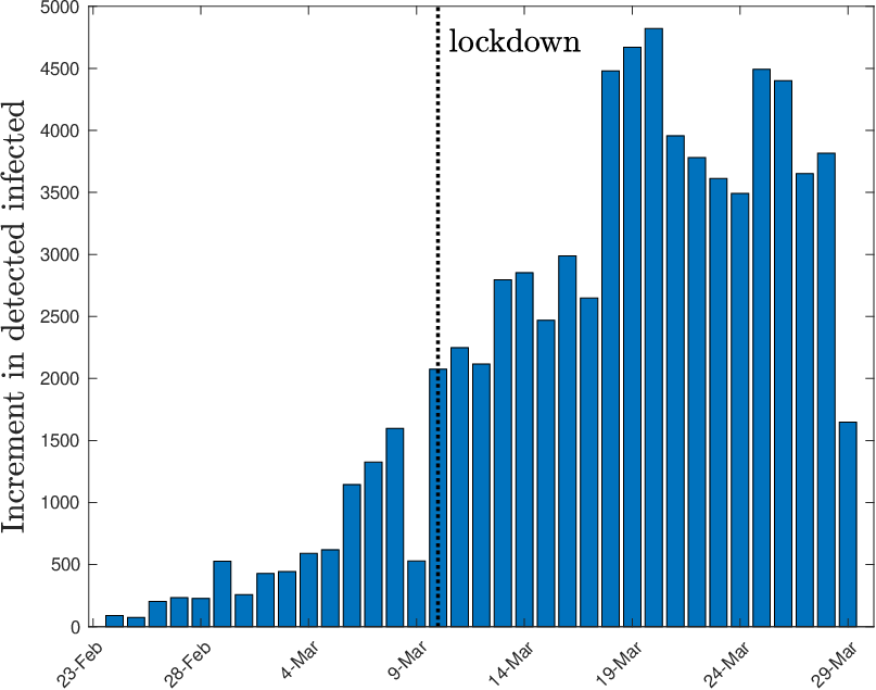
Finally, notice that the data we used for tuning the model run up to March 30th, 2020. As it can be seen in Figure 3 most recent data show a substantial decrease of the number of infected individuals, which is imputable to the coming into effect, after a delay of about two weeks, of the lockdown measures imposed by the government. Clearly, the underlying process is non-stationary, and the predictions of the model tuned using data up to March 30th, 2020 will (hopefully) be pessimistic, as the lockdown will drastically change the underlying mechanics of the contagion.


References
- [1] G. Chowell, “Fitting dynamic models to epidemic outbreaks with quantified uncertainty: A primer for parameter uncertainty, identifiability, and forecasts,” Infectious Disease Modelling, vol. 2, no. 3, pp. 379–398, 2017.
- [2] W. Kermack and A. McKendrick, “A contribution to the mathematical theory of epidemics,” Proceedings of the Royal Society of London, vol. A 115, pp. 700–721, 1927.
- [3] F. J. Richards, “A flexible growth function for empirical use,” Journal of Experimental Botany, vol. 10, no. 2, pp. 290–301, 1959.
- [4] G. Chowell, A. Tariq, and J. M. Hyman, “A novel sub-epidemic modeling framework for short-term forecasting epidemic waves,” BMC Medicine, vol. 17, no. 1, p. 164, 2019.
- [5] N. T. J. Bailey, The mathematical theory of infectious diseases and its applications. New York, NY, USA: Hafner Press, 2nd ed., 1975.
- [6] F. Brauer, “Mathematical epidemiology: Past, present, and future,” Infectious Disease Modelling, vol. 2, no. 2, pp. 113–127, 2017.
- [7] M. J. Keeling and K. T. Eames, “Networks and epidemic models,” Journal of the Royal Society Interface, vol. 2, no. 4, pp. 295–307, 2005.
- [8] M. Nadini, A. Rizzo, and M. Porfiri, “Epidemic spreading in temporal and adaptive networks with static backbone,” IEEE Transactions on Network Science and Engineering, vol. 7, no. 1, pp. 549–561, 2020.
- [9] C. Nowzari, V. M. Preciado, and G. J. Pappas, “Optimal resource allocation for control of networked epidemic models,” IEEE Transactions on Control of Network Systems, vol. 4, no. 2, pp. 159–169, 2015.
- [10] R. Pastor-Satorras, C. Castellano, P. Van Mieghem, and A. Vespignani, “Epidemic processes in complex networks,” Reviews of modern physics, vol. 87, no. 3, p. 925, 2015.
- [11] A. Y. Pastore Piontti, M. F. D. C. Gomes, N. Samay, N. Perra, and A. Vespignani, “The infection tree of global epidemics,” Network Science, vol. 2, no. 1, pp. 132–137, 2014.
- [12] L. Pellis, F. Ball, S. Bansal, K. Eames, T. House, V. Isham, and P. Trapman, “Eight challenges for network epidemic models,” Epidemics, vol. 10, pp. 58–62, 2015.
- [13] J. O. Wertheim, A. J. Leigh Brown, N. L. Hepler, S. R. Mehta, D. D. Richman, D. M. Smith, and S. L. Kosakovsky Pond, “The global transmission network of HIV-1,” Journal of Infectious Diseases, vol. 209, no. 2, pp. 304–313, 2014.
- [14] K. Mizumoto, K. Kagaya, A. Zarebski, and G. Chowell, “Estimating the asymptomatic proportion of coronavirus disease 2019 (COVID-19) cases on board the Diamond Princess cruise ship, Yokohama, Japan, 2020,” Eurosurveillance, vol. 25, no. 10, p. 2000180, 2020.
- [15] W. Gleissner, “The spread of epidemics,” Applied Mathematics & Computation, vol. 27, pp. 167–171, 1988.
- [16] S. Boyd and L. Vandenberghe, Convex optimization. Cambridge, UK: Cambridge University Press, 2004.
- [17] S. Flaxman, S. Mishra, A. Gandy, et al., “Estimating the number of infections and the impact of non- pharmaceutical interventions on COVID-19 in 11 European countries,” tech. rep., Imperial College London, 2020.