Distance-based Formation Tracking with Unknown Bounded Reference Velocity
Abstract
TThis paper studies a distance-based formation tracking problem in the -dimensional space. The formation has a directed acyclic leader-following structure with leaders moving at a same unknown bounded velocity. Distributed control laws are proposed for follower agents to maintain the desired formation shape and move at the leaders’ velocity in finite time. Simulation results are also provided to support the theoretical analysis.
I Introduction
Formation-type collective behaviors such as bird flocking, fish schooling, or V-shaped flying formation are frequently observed in nature. A number of research works suggests that formation-type collective behaviors serve survival needs of animals (evading predator, hunting, foraging, etc.) and these behaviors require the individuals to interact or communicate with each other. Inspired by formation-type behaviors, formation control has been extensively studied. Beyond theoretical meaning, formation control also finds applications in satellite formations, robotics, and sensor networks [1].
Formation control can be categorized into several categories: position-, displacement-, distance-, bearing vector-, angle-, and mixed-sensing based approaches [2]. The difficulties of these approaches mainly depend on the amount of information that each agent can be accessed to solve the problem. Since position- and displacement- based approaches require knowledge of the global reference frame [3], bearing- and angle-based approaches have no control on formation’s scale [4], the distance-based approach has been the focus of many research works [5, 6, 7, 8, 9]. In distance-based formation control, each agent senses the relative positions of its neighboring agents in its local reference frame [10] and control some desired distances with other agents. As a result, there is no need of a global reference coordinate system. However, the lack of global information makes the control design and analysis of this approach more challenging.
Existing works on distance-based formation control mostly focused on the formation acquisition process using gradient descent control laws [11, 12]. The distance-based formation tracking problem is more challenging because the agents have to achieve the desired formation shape and follow a reference trajectory simultaneously. In [13], an undirected formation tracking problem was studied, where the authors introduced a nonlinear PI controller so that the agents can track a leader moving at a constant velocity. The authors in [10] studied a directed leader-follower formation and proposed a velocity estimator to estimate the leaders’ velocities. However, the velocity estimator in [10, 2] is applicable when the leaders’ velocity is constant or vanishing exponentially fast. The authors in [14] studied a distance-based problem where the reference velocity of the formation centroid is estimated (by a finite-time consensus algorithm) and tracked by all agents. Finally, formation control with bounded disturbances has been also recently studied in [15, 16].
In this paper, we study a distance-based formation tracking problem for single-integrator modeled agents in . There are leaders moving with the same bounded reference velocity. The remaining agents, called followers, can measure the relative positions of neighboring agents in their local reference frame and only know an upper bound of the reference velocity. The sensing/controlling topology among agents in the formation is described by a directed acyclic graph. Then, there exists a first follower agent, whose neighbors are leaders. A finite-time control law is proposed so that the first follower can achieve all the desired distances with regard to the leaders and follow the leader’s velocity at the same time. The proposed control law consists of two components: the first component drives the agent to a time varying desired position in a finite time and the second component tracks the unknown reference velocity. It is noted that the finite-time formation control component in this paper is different from existing ones in the literature [17, 18, 19]. As the leader’s velocity is unknown to the follower, their movements are considered as disturbances acting on the follower’s motion. Thus, the second component of our control law, which includes a signum function, is included to eliminate the effect of the leaders’ movement to the formation. As the formation has a leader-following structure, the stability analysis starts from the first follower, whose neighbors are the leaders. After the first follower achieved all desired distances and moved at the same velocity with the leaders, it can be considered as a new leader, and the local stability of the formation follows from mathematical induction.
The remainder of this paper is organized as follows. Section 2 provides the related background and main assumptions before formulating the main problem studied in this paper. The proposed control law and stability analysis are presented in Section 3. Simulation results are given in Section 4, and Section 5 concludes the paper.
II Preliminaries
II-A Notation
In this paper, , and denote the set of real numbers, the -dimensional Euclidean space and the set of real matrices, respectively. , , and denote the 1-, 2-, and -norm of a vector. Let be a vector in . Denote , and , where and is the signum function. , , , and denote the determinant, the Frobenius norm, the vectorization operation, and the Hadamard product, respectively.
II-B Problem Formulation
Consider a system of single-integrator agents in the -dimensional space (). Let ,…, denote the positions of the agents written in a global reference frame. Let and be sets of leaders and followers. Suppose that in the system, leader agents have knowledge about the global reference frame and they are moving with the same reference velocity. More specifically, the leaders’ motions are governed by the equations where is assumed to be a bounded, continuous reference velocity which is the same for all leaders. The other agents are followers and each follower maintains a local reference frame . The motion of a follower can be expressed in its local reference frame as follows: where and are the position of agent and its control input expressed in , respectively. The relative position of agent with regard to agent in , or the local displacement between and , is defined as . Further, we denote as the displacement written in . The distance between and is denoted by .
A directed graph is used to characterize the interaction among the agents in the system, where is the set of nodes and is the set of edges. Each node in represents an agent in the system. The neighbor set of node is defined as . Then, or means that agent senses the relative position of agent with respect to and controls the distance between them.
In this paper, we consider formations having a leader-following sensing/controlling graph constructed by the following procedure, which is called Procedure 1:
- •
Start with vertices .
- •
For , add a vertex together with directed edges to the current graph, where .
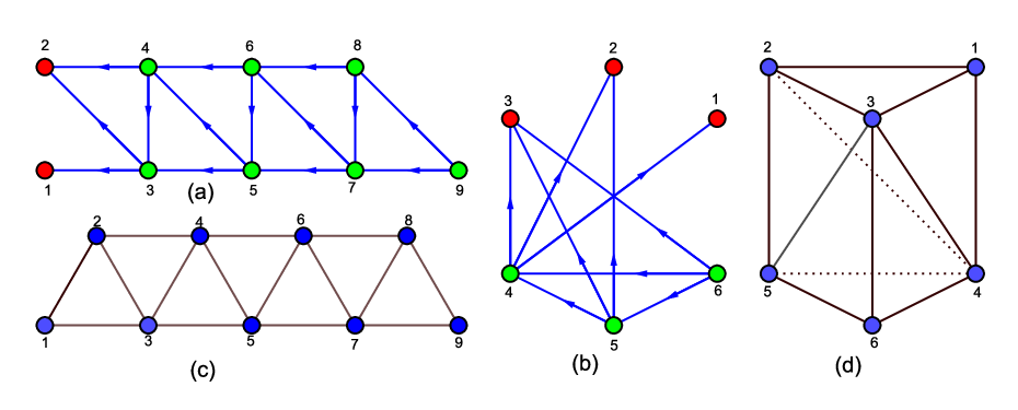
Example of graphs constructed from Procedure 1 are given in Fig. 1.
From the construction of , it is clear that is directed and acyclic. Furthermore, for each follower , and . Next, define , where .
A formation is defined by , where characterizes the distance constraints between agents and is a realization of in . The realization induces a set of realizable distance constraints . Conversely, a set is realizable if there exists a realization satisfying all the distance constraints in .
Two realizations and of are congruent if and only if , . A realization is rigid if there exists such that all realizations of the distance set induced by and satisfying are congruent to . The graph is generically rigid if almost all realizations of are rigid [5, 20]. The following assumptions will be adopted in this paper:
Assumption 1.
The graph is constructed from Procedure 1. The graph is generically rigid.
Assumption 2.
The set of desired distances is realizable and there exists a desired realization of which is rigid.
Assumption 3.
The leaders are initially positioned at such that and they move at the same velocity , where is an unknown continuous vector function in such that . The initial positions of each follower and its neighbors are not degenerate in .
Assumptions 2 and 3 imply that for any , the dimension of the affine span of and for is . The problem studied in this paper is stated as follows:
Problem.

III Main Results
III-A Proposed control laws
Consider the first follower . For an arbitrary number , we propose the following control law written in the local reference frame of agent :
| (1) |
where are the squared distance errors and is a constant number. In (1), the component is used to achieve the desired distances in a finite time and the component handles the uncertainty in the leaders’ velocity. The control law (1) is distributed since each agent uses only the relative positions of its neighboring agents.
III-B Stability analysis
Denote , , , where . Let and .
Theorem 1.
Under the control law (1), approaches the set as . Moreover, is bounded.
Proof.
We denote the leaders’ velocity in the reference frame of agent by . There exists a rotation matrix such that . Thus, the following inequality holds Consider the positive definite Lyapunov function It follows from the chain rule [21] that
| (2) |
where
| (3) |
Note that , substituting this result into (2) yields
Based on the vector norm inequalities, we obtain
| (4) |
Therefore, is evaluated as follows
| (5) |
which implies tends to as . Furthermore, the boundedness of can be obtained from (5) as follows
| (6) |
From (6) and the definition of , we have and are also bounded for all , which leads to the boundedness of . Thus, combining with the fact that is bounded, we conclude is bounded. ∎
Note that distance errors and are invariant with a change of the coordinate frame. Consider the reference frame which moves at the leaders’ velocity. In , the leaders do not move and we can determine the value of if in , for example in , as follows. Suppose the origin of is the middle point of two leaders of (i.e., and ). Denote , , and by , , as can be seen in Fig. 2. From the definition of and , it is clear that if and only if and
Therefore, the set can be determined and its cardinality is finite (less than 4), so we can calculate . This number is denoted by . Note that only depends on the desired distances. From definitions of and , it is clear that and are the sets of global minimum extrema and potential extrema of the function , which implies that is the smallest local minimum value of . Therefore, the condition means that the initial value of is less than its smallest local minimum value, which leads to the fact that tends to the global minimum value as because is nonincreasing. We have the following theorem regarding this fact.
Theorem 2.
Under the control law (1), if then in finite time. After that time, the velocity of agent is equal to the leader’s velocity.
Proof.
Using (6), we have , and it follows that does not tend to . As a result, tends to as .
Let be an arbitrary number in . Since , we have . Moreover, the determinant is continuous, so . Consequently, there exists a positive number such that if . This inequality implies .
Since the matrix is symmetric and positive definite when , all eigenvalues of are positive. Let be the minimum eigenvalue of and let be its the remaining eigenvalues. From the structure of the matrix , there holds Thus, the following result is obtained
It follows that which leads to the following evaluation
| (7) |
Hence, in the set .
Because approaches to as , will converge into the set after a finite time . Equation (6) shows that is a nonincreasing function, so . Hence, the trajectory does not escape from . Thus, Based on this and (5), can be evaluated as follows
| (8) |
Denote and , we will prove that Suppose . Because is nonincreasing and nonnegative, we obtain . Hence, the continuity of and shows that is continuous in . This implies the existence of . Therefore,
| (9) |
This contradiction implies . Since is a nonnegative and nonincreasing function, it follows that , and this implies that the control law drives the agent to the desired position in a finite time . We have , if and only if , . Taking the derivative of for , we have , where is the velocity of agent . It follows that . Because the matrix is nonsingular, we have . ∎
Remark 1.
Under the proposed control law, for , the agent satisfies all desired distance constraints and has the same velocity as the leaders. After that, it is possible to consider agent as a leader to control the next follower. Thus, the problem of controlling subsequent followers can be solved similarly and the stability of the -agent formation follows from mathematical induction.
Remark 2.
To decrease the convergence time, we can modify (1) as follows:
| (10) |
where , and . Under the control law (10), by a similar analysis, (8) becomes
| (11) |
where and are two strictly positive real numbers. It can be seen that in (11), when is quite large, the component dominates and makes decreases fast until . After , the component becomes bigger and makes converge to in finite time.
Remark 3.
Let we assume the velocity function of the leaders is given by
| (12) |
where is an unknown continuous matrix function in satisfying , where is a known constant, and is a known bounded continuous function. The proposed control law in this case is similar to (1), except that the term becomes , that is,
| (13) |
Similar to Remark 2, we can also use the following control law to decrease the convergence time
| (14) |
Theorem 2 is still correct under these proposed control laws (13) and (14).
IV Simulation Results
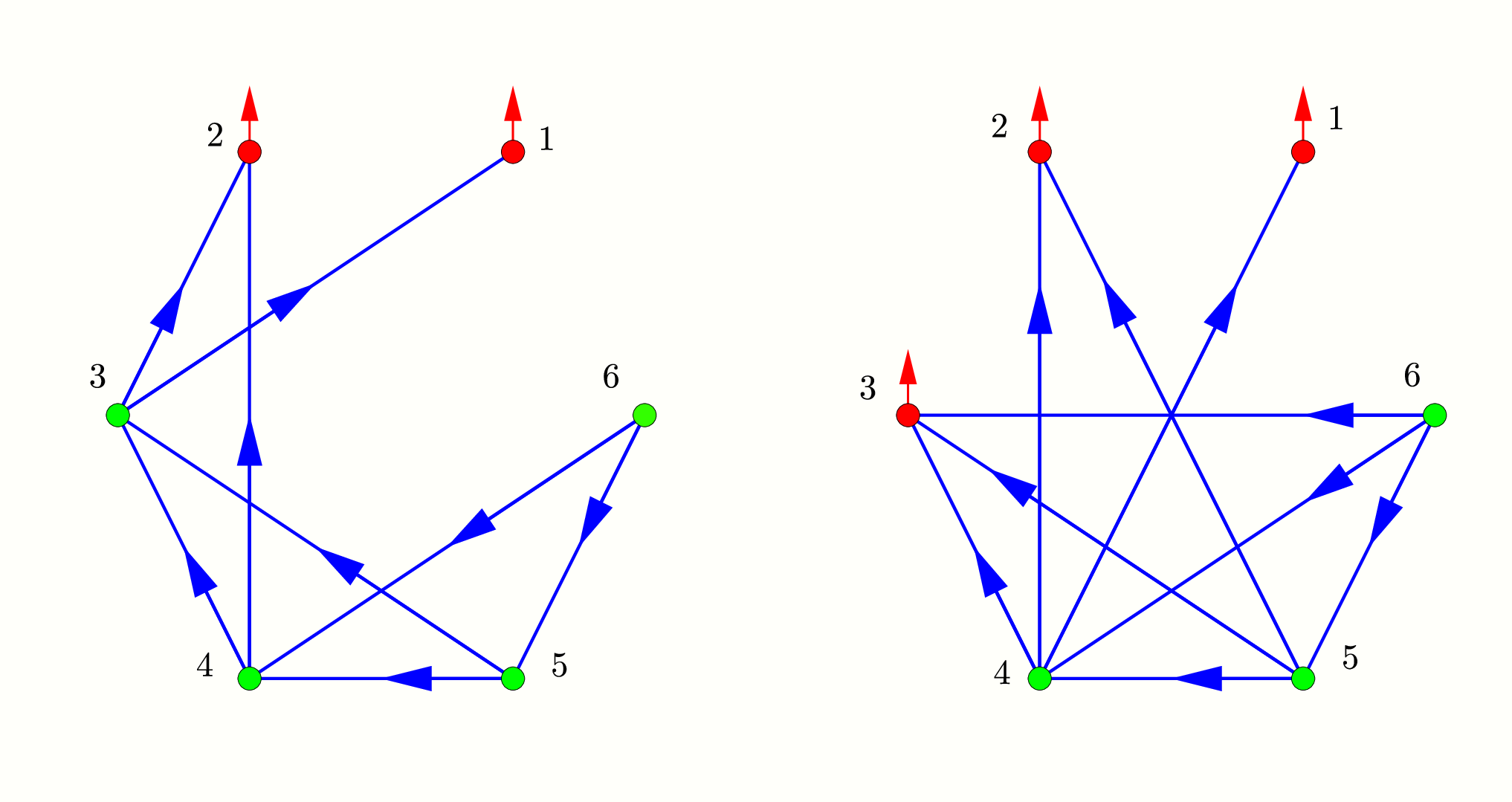
In this section, we conduct two simulations to validate the theoretical results in Section 3. In Simulation 1, we consider a nine-agent system in (2 leaders and 7 followers) and in Simulation 2, we consider a six-agent system in (3 leaders and 3 followers). The graphs are constructed by Procedure 1, e.g., in Simulation 1, the leader-follower graph is defined as , where and . The graphs and the desired formations in two simulations are depicted in Fig. 3. The orientation and initial positions of the followers are randomly generated.
IV-A Simulation 1
In this simulation, the control law (1) is adopted for the agents. The parameters are chosen as follows: , , . The initial positions of two leaders are and . The desired distances are all chosen as . The leaders’ velocity is , where and were randomly selected.
Trajectories of nine agents and the squared distance errors are depicted in Fig. 4. As can be seen in Fig. 4, for s, are all zero. The agents then have the same velocity, and thus the formation shape is maintained after that.


IV-B Simulation 2
In this simulation, the initial positions of three leaders are , , and . The desired distances are and . Therefore, the desired formation is an uniform triangular prism. With arbitrary numbers , the matrix and the vector in Remark 3 are chosen as
| (15) |
and . The control laws (13) with is adopted for Simulation 2a and the control law (14) with is adopted in Simulation 2b.
Figure 5 depicts the trajectories of agents and the squared distance errors versus time. We also observe that the desired formation is achieved in a finite time, and the agents move at the same velocity after that. Moreover, by comparing the squared distance errors vs time in Simulations 2a and 2b, we also observe that the convergence time decreases when (14) is adopted.
V Conclusions
In this paper, the distance-based formation tracking problem was studied for formations with the leader-following topology. The proposed control law guarantees the followers to maintain the desired distances with regard to its leaders and move at the same velocity with the leader after a finite time. Simulation results were also provided to accompanied with the analysis.


Acknowledgment
This work was supported by the National Research Foundation of Korea (NRF) under the grant NRF- 2017R1A2B3007034.
References
- [1] B. D. O. Anderson, C. Yu, B. Fidan, and J. M. Hendrickx, “Rigid graph control architectures for autonomous formations,” IEEE Control Systems Magazine, vol. 28, no. 6, pp. 48–63, 2008.
- [2] H.-S. Ahn, Formation Control: Approaches for distributed agents. Springer, 2020.
- [3] K.-K. Oh, M.-C. Park, and H.-S. Ahn, “A survey of multi-agent formation control,” Automatica, vol. 53, pp. 424–440, 2015.
- [4] S. Zhao and D. Zelazo, “Bearing rigidity and almost global bearing-only formation stabilization,” IEEE Transactions on Automatic Control, vol. 61, no. 5, pp. 1255–1268, 2016.
- [5] J. M. Hendrickx, B. D. O. Anderson, J.-C. Delvenne, and V. D. Blondel, “Directed graphs for the analysis of rigidity and persistence in autonomous agent systems,” International Journal of Robust and Nonlinear Control, vol. 17, no. 10-11, pp. 960–981, 2007.
- [6] K.-K. Oh and H.-S. Ahn, “Formation control of mobile agents based on inter-agent distance dynamics,” Automatica, vol. 47, no. 10, pp. 2306–2312, 2011.
- [7] Y.-P. Tian and Q. Wang, “Global stabilization of rigid formations in the plane,” Automatica, vol. 49, no. 5, pp. 1436–1441, 2013.
- [8] Z. Sun, S. Mou, B. D. O. Anderson, and M. Cao, “Exponential stability for formation control systems with generalized controllers: A unified approach,” Systems & Control Letters, vol. 93, pp. 50–57, 2016.
- [9] M. H. Trinh, V. H. Pham, M.-C. Park, Z. Sun, B. D. O. Anderson, and H.-S. Ahn, “Comments on “Global stabilization of rigid formations in the plane [automatica 49 (2013) 1436–1441]”,” Automatica, vol. 77, pp. 393–396, 2017.
- [10] S.-M. Kang, M.-C. Park, B.-H. Lee, and H.-S. Ahn, “Distance-based formation control with a single moving leader,” in 2014 American Control Conference. IEEE, 2014, pp. 305–310.
- [11] Z. Sun, U. Helmke, and B. D. O. Anderson, “Rigid formation shape control in general dimensions: an invariance principle and open problems,” in Proc. of the 54th IEEE Conference on Decision and Control (CDC). IEEE, 2015, pp. 6095–6100.
- [12] M. Cao, B. D. O. Anderson, A. S. Morse, and C. Yu, “Control of acyclic formations of mobile autonomous agents,” in 2008 47th IEEE Conference on Decision and Control. IEEE, 2008, pp. 1187–1192.
- [13] O. Rozenheck, S. Zhao, and D. Zelazo, “A proportional-integral controller for distance-based formation tracking,” in 2015 European Control Conference (ECC). IEEE, 2015, pp. 1693–1698.
- [14] Q. Yang, M. Cao, H. Fang, and J. Chen, “Weighted centroid tracking control for multi-agent systems,” in Prof. of the IEEE 55th Conference on Decision and Control (CDC). IEEE, 2016, pp. 939–944.
- [15] F. Mehdifar, C. P. Bechlioulis, F. Hashemzadeh, and M. Baradarannia, “Prescribed performance distance-based formation control of multi-agent systems,” arXiv preprint arXiv:1911.07266, 2019.
- [16] D. V. Vu, M. H. Trinh, P. D. Nguyen, and H.-S. Ahn, “Distance-based formation control with bounded disturbances,” IEEE Control Systems Letters, vol. 5, no. 2, pp. 451–456, 2021.
- [17] M.-C. Park, Z. Sun, K.-K. Oh, B. D. O. Anderson, and H.-S. Ahn, “Finite-time convergence control for acyclic persistent formations,” in 2014 IEEE International Symposium on Intelligent Control (ISIC). IEEE, 2014, pp. 1608–1613.
- [18] Z. Sun, S. Mou, M. Deghat, B. D. O. Anderson, and A. S. Morse, “Finite time distance-based rigid formation stabilization and flocking,” IFAC Proceedings Volumes, vol. 47, no. 3, pp. 9183–9189, 2014.
- [19] V. H. Pham, M. H. Trinh, and H.-S. Ahn, “Finite-time convergence of acyclic generically persistent formations,” in 2018 Annual American Control Conference (ACC). IEEE, 2018, pp. 3642–3647.
- [20] C. Yu, J. M. Hendrickx, B. Fidan, B. D. O. Anderson, and V. D. Blondel, “Three and higher dimensional autonomous formations: Rigidity, persistence and structural persistence,” Automatica, vol. 43, no. 3, pp. 387–402, 2007.
- [21] D. Shevitz and B. Paden, “Lyapunov stability theory of nonsmooth systems,” IEEE Transactions on automatic control, vol. 39, no. 9, pp. 1910–1914, 1994.