Initial results from a realtime FRB search with the GBT2020Initial results from a realtime FRB search with the GBT–References

Devansh Agarwal Thanks: da0017@mix.wvu.edu Affiliation: West Virginia University, Department of Physics and Astronomy, P. O. Box 6315, Morgantown, WV, USA Affiliation: Center for Gravitational Waves and Cosmology, West Virginia University, Chestnut Ridge Research Building, Morgantown, WV, USA D. R. Lorimer Affiliation: West Virginia University, Department of Physics and Astronomy, P. O. Box 6315, Morgantown, WV, USA Affiliation: Center for Gravitational Waves and Cosmology, West Virginia University, Chestnut Ridge Research Building, Morgantown, WV, USA M.P. Surnis Affiliation: West Virginia University, Department of Physics and Astronomy, P. O. Box 6315, Morgantown, WV, USA Affiliation: Center for Gravitational Waves and Cosmology, West Virginia University, Chestnut Ridge Research Building, Morgantown, WV, USA X. Pei Affiliation: Xinjiang Astronomical Observatory, Chinese Academy of Sciences, Urumqi, Xinjiang 830011, China Affiliation: University of Chinese Academy of Sciences, Beijing 100049, China A. Karastergiou Affiliation: University of Oxford, Sub-Department of Astrophysics, Denys Wilkinson Building, Keble Road, Oxford, OX1 3RH, United Kingdom Affiliation: Physics Department, University of the Western Cape, Cape Town 7535, South Africa Affiliation: Department of Physics and Electronics, Rhodes University, PO Box 94, Grahamstown 6140, South Africa G. Golpayegani Affiliation: West Virginia University, Department of Physics and Astronomy, P. O. Box 6315, Morgantown, WV, USA Affiliation: Center for Gravitational Waves and Cosmology, West Virginia University, Chestnut Ridge Research Building, Morgantown, WV, USA D. Werthimer Affiliation: Department of Astronomy, University of California, Berkeley, 501 Campbell Hall #3411, Berkeley, CA 94720, USA J. Cobb Affiliation: Department of Astronomy, University of California, Berkeley, 501 Campbell Hall #3411, Berkeley, CA 94720, USA M.A. McLaughlin Affiliation: West Virginia University, Department of Physics and Astronomy, P. O. Box 6315, Morgantown, WV, USA Affiliation: Center for Gravitational Waves and Cosmology, West Virginia University, Chestnut Ridge Research Building, Morgantown, WV, USA S. White Affiliation: Green Bank Observatory, P.O. Box 2, Green Bank, WV 24944, USA W. Armour Affiliation: OeRC, Department of Engineering Science, University of Oxford, Keble Road, Oxford OX1 3QG, UK D.H.E. MacMahon Affiliation: Department of Astronomy, University of California, Berkeley, 501 Campbell Hall #3411, Berkeley, CA 94720, USA A.P.V. Siemion Affiliation: Department of Astronomy, University of California, Berkeley, 501 Campbell Hall #3411, Berkeley, CA 94720, USA Affiliation: Radboud University, Nijmegen, 6525 HP, the Netherlands Affiliation: SETI Institute, Mountain View, CA 94043, USA G. Foster Affiliation: University of Oxford, Sub-Department of Astrophysics, Denys Wilkinson Building, Keble Road, Oxford, OX1 3RH, United Kingdom

Accepted XXX. Received YYY; in original form ZZZ

Abstract

We present the data analysis pipeline, commissioning observations and initial results from the GREENBURST fast radio burst (FRB) detection system on the Robert C. Byrd Green Bank Telescope (GBT) previously described by Surnis et al. which uses the 21 cm receiver observing commensally with other projects. The pipeline makes use of a state-of-the-art deep learning classifier to winnow down the very large number of false positive single-pulse candidates that mostly result from radio frequency interference. In our observations totalling 156.5 days so far, we have detected individual pulses from 20 known radio pulsars which provide an excellent verification of the system performance. We also demonstrate, through blind injection analyses, that our pipeline is complete down to a signal-to-noise threshold of 12. Depending on the observing mode, this translates to peak flux sensitivities in the range 0.14–0.89 Jy. Although no FRBs have been detected to date, we have used our results to update the analysis of Lawrence et al. to constrain the FRB all-sky rate to be $1140^{+200}_{-180}$ per day above a peak flux density of 1 Jy. We also constrain the source count index $\alpha=0.83\pm 0.06$ which indicates that the source count distribution is substantially flatter than expected from a Euclidean distribution of standard candles (where $\alpha=1.5$ ). We discuss this result in the context of the FRB redshift and luminosity distributions. Finally, we make predictions for detection rates with GREENBURST, as well as other ongoing and planned FRB experiments.

Keywords:

radio continuum: transients – surveys – stars: pulsars: general

1 Introduction

Fast Radio bursts (FRBs) are enigmatic astrophysical objects that burst for millisecond durations with flux densities of the order of a few Jansky that were first discovered by Lorimer et al. 2007. FRBs show the characteristic inverse frequency squared sweep in observing frequency, which is quantified by the dispersion measure (DM). Their DMs are substantially larger than those expected from the Milky Way in the direction of detection, indicating their extragalactic nature. To date, $\sim$ 110 FRBs have been reported¹¹ 1 http://frbcat.org (see Petroff et al. 2016, and references therein), and their origins are still unclear. Out of all the FRBs discovered so far, of special interest are those which show repeat bursts. The first repeater, FRB 121102, (Spitler et al. 2014) was localised to a host galaxy by Chatterjee et al. 2017. FRB 171019 was found to have repeat bursts with $\sim 350$ times smaller fluence as compared to the first detection (Shannon et al. 2018; Kumar et al. 2019) and 18 repeaters were also recently reported (The CHIME/FRB Collaboration et al. 2019a; The CHIME/FRB Collaboration et al. 2019b; Fonseca et al. 2020a). Very recently, a 16.34-day periodicity from the repeating FRB 180916.J0158+65 (Collaboration et al. 2020) and a possible 159-day periodicity for FRB 121102 (Rajwade et al. 2020) were announced.

Detection of FRBs requires data at radio frequency to be de-dispersed at many trial DM values. For each DM, all the frequencies are added to form a time series which is then searched using matched filters to find bursts above a certain threshold. With the help of Graphics Processing Units (GPUs), it is now possible to perform such searches in real time (Magro et al. 2011; Barsdell et al. 2012; Karastergiou et al. 2015; Adamek & Armour 2019). Inspired by the capabilities of real-time processing which has been successfully implemented at Parkes (see Osłowski et al. 2019, for recent commensal discoveries), many radio telescopes around the globe are deploying commensal search backends to enable serendipitous discoveries of FRBs. A few examples include: realfast (Law et al. 2018) at the Very Large Array, the craft survey with the Australian Square Kilometre Array Pathfinder (ASKAP) telescope (Macquart et al. 2010), alfaburst at the Arecibo observatory (Chennamangalam et al. 2017a; Foster et al. 2017) and GBTrans using the 20 m telescope at Green Bank (Golpayegani et al. 2019). With such backends, a copy of the data from the receiver is de-dispersed and searched for FRBs. Real-time detection of FRBs is required for prompt follow-up at other wavelengths that might provide valuable insights towards understanding the underlying emission mechanisms and possible progenitors.

In this paper we present the results from 3756 hours on sky from the commensal backend at the 110 m Robert C. Byrd Green Bank Telescope (GBT). We henceforth refer to this system as GREENBURST. This paper is organised as follows. We first describe and summarise the system description and detail the FRB search pipeline in §2 followed by benchmarks of our pipeline in §3. In §4 we present results from our commensal observations and constraints on FRB rates. In §5, we discuss the consequences of our results in terms of FRB source counts and predictions for ongoing future experiments. Finally, in §6, we present our conclusions.

2 Search Pipeline

Figure 1: Schematic depiction of the detection pipeline. Data through ethernet arrives as user datagram protocol (UDP) packets. Using a double buffer system, data from the UDP packets are rearranged and written in filterbank format. In parallel, all the telescope metadata are saved in the influx database at 1 s intervals. Once a filterbank file is written, data validity is checked (see text for details). Valid data are searched with heimdall. Candidates are then parsed through FETCH, and positively labelled candidates are sent for visual inspection. A condensed version of telescope metadata and the candidates is saved in elasticsearch for future reference.

The system description is detailed in Surnis et al. 2019 and is summarised here. Using a dedicated directional coupler designed and built at the observatory, we obtain a copy of the signal from the L-band (21 cm) receiver. This signal is then digitised using a field programmable gate array on board the setiburst backend (Chennamangalam et al. 2017b) and sampled every 256 $\mu$ s with 8-bit precision. The resulting data stream consists of 4096 channels spanning a 960 MHz bandwidth at a central frequency of 1440 MHz. A unique property of this system is that even when the L-band receiver is not in the primary focus, it still is illuminated by a large part of the dish. As a result, it can be used commensally with observations at other frequencies.

Fig. 1 details our search and verification pipeline. The digitised data are transported over an ethernet connection to a dedicated computer which processes and stores the data as binary files in filterbank format (Lorimer et al. 2000). The filterbank files contain 16 chunks of $2^{17}$ samples corresponding to 10,000 $\text{pc}\;\text{cm}^{-3}$ DM delay along with an overlapping chunk from the last file. The overlap ensures that no transient events are missed due to data being split between two files. In parallel, the telescope metadata, which includes the receiver turret angle, telescope pointing altitude and azimuth, and observing project IDs are recorded at a cadence of one second in influxDB²² 2 https://www.influxdata.com. This serves as a high-resolution short term storage database, where the metadata are saved for seven days.

Refer to caption — Figure 2: Radio frequency interference clipping using the Savitzky–Golay filter. The bottom left, and middle plots show the raw and cleaned de-dispersed spectrum of a single from PSR B0329+54. In the bottom right panel, the raw bandpass is shown in blue, while the smoothed bandpass from the filter is shown by the black dashed lines. The red lines mark the flagged channels. The top left and middle plots show the frequency integrated profile of the single pulse.

Once a filterbank file is written, data validity is checked using metadata from influxDB. The data are considered invalid if any of the following conditions are met.

•

The receiver turret is unlocked. This typically happens when the observer changes the receiver in focus.
•

The turret angle is between 160^∘ and 220^∘. At these angles the GBT primary focus feed structure blocks the receiver’s field of view.
•

The primary focus receiver is extended due to the same reason as above.

If the data are valid, we first excise radio frequency interference (RFI) from affected channels using the following method. All the time samples are added to form a bandpass of the data. The bandpass is smoothed using a Savitzky--Golay filter. Here we use a running window of 61 data samples and fit a second-order polynomial to obtain a smooth bandpass. The measured and smooth bandpass are subtracted from one another. Through empirical investigations with preliminary data, we found that a good RFI excision procedure is to use this subtraction result and flag any channels which differ from the smooth bandpass by more than five counts³³ 3 Here we use the term “count” to refer to an intensity value quantized in the range 0–255. Five counts corresponds to $\sim 6$ times the root mean square value of the data.. Both the window size and the difference threshold were determined empirically. Fig. 2 shows the profile of PSR B0329+54, before and after masking bad channels. In parallel, a coarse version of the telescope metadata is computed by binning by time spent by the telescope in each 1 ${}^{\circ}\times$ 1^∘ patch in the Galactic latitude-longitude grid. The metadata are subsequently used to generate sky coverage maps and rate calculations of FRBs described below.

We use heimdall⁴⁴ 4 https://sourceforge.net/projects/heimdall-astro along with the bad channel flags to search for pulses in the range $10\leq$ DM $\leq 10,000$ $\text{pc}\;\text{cm}^{-3}$ , and smoothing over $[2^{0},2^{1},...,2^{7}]$ adjacent samples spanning widths in the range 256 $\mu$ s—32.768 ms above a signal to noise ratio (S/N) of 8. The candidates above the S/N threshold are then classified as either RFI or an astronomical transient using model a of the artificial neural network FETCH (Agarwal et al. 2019a). Candidates labelled as positives are then sorted into two categories: Galactic and extragalactic. We do this by computing the expected DM contribution in the direction of observation by integrating the electron density by both NE2001 and YMW16 models out to 25 kpc. The smaller of the two DM estimates is chosen as the Galactic DM in that direction. In case the candidate DM is Galactic, the position and DM are matched with the ATNF pulsar catalogue (Manchester et al. 2005) to verify if the candidate is a known source. If the source is unknown or the DM is larger than the Galactic DM, the candidates are marked for manual verification. Positively marked candidates are stored in the elasticsearch⁵⁵ 5 https://www.elastic.co/elasticsearch database.

3 Pipeline Benchmarks

To assess the completeness of our pipeline, we injected fake FRBs with various observational parameters and run the complete pipeline as detailed in §2. Based on the results from our pipeline we compute several metrics to quantify the pipeline’s ability to detect FRBs.

3.1 Blind FRB injections

Table 1: Distributions of FRBs injected for benchmarking the pipeline

Parameter name	Distribution
Signal-to-noise ratio	Uniform(6,100)
Pulse width	Uniform(0.5, 26) ms
Spectral index	Uniform(–3,3)
Scattering time	Uniform(0.256,6.5) ms
Number of scintillation patches	Log-Uniform(–3, 2)

To inject FRBs, we first randomly select filterbank files from the observations on a single day (MJD 58728). On this date, all the data were acquired using the L-band receiver. The parameters of the injected FRB distribution are summarised in Table 1. For each injection, first a random start time in the file is chosen such that there is enough data to fully inject the dispersion delay. Then, Gaussian-shaped profiles are created for each channel with standard deviation

w=\sqrt{t_{\text{samp}}^{2}+t_{\text{DM}}^{2}+w_{\text{int}}^{2}}.

(1)

Here $t_{\text{samp}}=256~\mu$ s is the sampling interval, $t_{\text{DM}}$ is the dispersion smearing (the delay due to dispersion across a channel bandwidth) and $w_{\text{int}}$ is the intrinsic pulse width drawn from a uniform distribution between 0.5 and 26 ms. This profile is then convolved with an exponential function of the form $e^{-t/\tau}/\tau$ , where $\tau$ is randomly drawn from a uniform distribution of 0.256 and 6.5 ms, to add scattering the the profile. The lower limit is 0.256 ms and not zero because of the $1/\tau$ normalisation factor and the upper limit of 6.5 ms such that the resultant widths of the scattered FRBs are similar to the observed population. These profiles are then scaled with the spectral index by multiplying with $(F/F_{\text{ref}})^{\gamma}$ . Here $F$ is the channel frequency, $F_{\text{ref}}$ is the reference frequency of 1400 MHz and $\gamma$ is the spectral index. Scintillation is added to the data by modulating the spectra using the positive half of a cosine function. The number of such patches are drawn from a log-normal distribution of mean –3 and standard deviation of 2. The above parameters lead to $\sim 10$ % of FRBs with a patchy spectral structure. To add scintillation we create an envelope where $N_{s}$ is the number of bright patches which is multiplied with the pulse. The envelope,

E=\cos\bigg[2\pi N_{s}\Big(\frac{F}{F_{\text{ref}}}\Big)^{2}+\phi\bigg],

(2)

is generated with $\phi$ being a random phase in the range 0 to $2\pi$ drawn from a uniform distribution. $E>0$ values are then multiplied with $S$ to simulate scintillation. The parameters from the above-described distributions are drawn and injected using the publicly available code injectfrb⁶⁶ 6 https://github.com/liamconnor/injectfrb. To create realistic bright FRBs, as our the data are 8-bit unsigned integers, for cases where the profile intensity exceeds the dynamic range the values are wrapped around the maximum value of 255. This is done because the FPGA wraps the numbers exceeding the dynamic range instead of clipping them at the maximum value. An instance of this can be viewed in Fig. 2 where dark blue patches can be seen within the dynamic spectrum of the pulsar.

3.2 Evaluation Metrics

Figure 3: The parameteric recall curve. The ordinate and abscissa correspond to the injected S/N and the recall respectively. The curve indicates that our pipeline is able to recover all the injected FRBs with S/N

\gtrsim

12.

To quantify the performance of our pipeline, we calculate what is known as “recall” (Sammut & Webb 2017) which is simply the ratio of the number of recovered FRBs to the total number of injected FRBs. While there are other metrics like accuracy and precision, their calculation involves the number of false positives which themselves depend on the RFI environment at the time of the observations and the performance of the RFI mitigation algorithms. We restrict our evaluation to the recovery of injected FRBs, and hence, we chose to evaluate using recall. To extract deeper insights than traditional recall, we here define a parameter weighted recall which we call parametric recall (PR). For this analysis we inject $\sim$ 1200 FRBs and we chose S/N as the parameter. Then, injected data are binned with respect to the parameter such that each bin has an equal number of points and the recall is calculated for each bin. PR can also be understood as the first moment of a distribution of recall over the given parameter. In this framework, we have

\text{PR}=\frac{\sum_{i=0}^{N_{\text{bins}}}\text{Recall}_{i}\,\mathcal{P}_{i}}{\sum_{i=0}^{N_{\text{bins}}}\mathcal{P}_{i}}.

(3)

Here, $\mathcal{P}_{i}$ and $\text{Recall}_{i}$ is the mean $\mathcal{P}$ and the recall of the $i^{\rm th}$ bin. The maximum value for the PR is unity, i.e. the pipeline found all FRBs at all injected S/N values. In case where the pipeline misses FRBs at high S/N the PR would be penalised more resulting in lower overall score. Hence PR is a better measure of performance as compared to traditional recall.

Fig. 3 shows the PR for the injected S/N as parameter ( $\mathcal{P}$ ). As can be seen from the plot, the pipeline is able to recover all events above a S/N $\sim$ 12. The PR from the above stated curve is 0.95. We inspected the candidates missed by the pipeline injected between a S/N of 8 to 12. All the candidates missed are due to the presence of strong RFI near the signal. In future, we plan to implement more sophisticated RFI mitigation algorithms to prevent achieve a lower S/N threshold with 100% reliability.

4 Results

GREENBURST started commensal observations on MJD 58587 (2019-03-14) and, as of MJD 58917 (2020-03-09), has observed for 156.5 days. While the backend has been operational for 330 days, only $\sim$ 50% of the available time has been spent on sky. This because of several factors that govern the validity of the data such as the telescope down time for maintenance, availability and observer’s choice of the receiver (see §2 for details).

Fig. 4 shows the sky coverage during this time in equatorial coordinates. The hexagons show $6^{\circ}\times 6^{\circ}$ area with colour bar representing the hours spent in the region.

Table 2: GREENBURST observational summary to date. From left to right, we list the receiver in prime focus, the turret angle relative to the L-band receiver, the time spent on sky with that receiver, the instantaneous solid angle covered

(\Omega)

and the sensitivity as evaluated from the blind injection analysis (see §3.1).

Receiver	Turret	Observation	$\Omega$	Sensitivity
	Angle	Time	$\times 10^{-2}$
	(^∘)	(hr)	(sr)	(Jy)
L-band	0	2194	3.12	0.14
X-band	260	615	3.33	0.89
C-band	60	556	3.19	0.25
Ku-band	100	210	3.40	0.80
MUSTANG	300	181	3.26	0.26

Table 2 shows the time spent, solid angle and sensitivity at each turret position for ${\rm S/N}=12$ . The sensitivity shown here is slightly different when compared to the numbers we reported earlier (Surnis et al. 2019) where we assumed a bandwidth of 960 MHz for the calculation and a S/N threshold of 12. Soon after the backend became functional, due to the presence of RFI, it was decided to always have the notch filter which blocks frequencies in the range 1.25–1.35 GHz in place. This filter is only taken out by the observer (primarily for pulsar/FRB observations). Along with the notch filter, we routinely flag $\sim$ 10% of the total band band reducing our bandwidth to 760 MHz. The beam solid angle, $\Omega\approx 1.33\,\text{FWHM}^{2}$ , where FWHM is the full width at half maximum and is taken from Surnis et al. 2019.

Table 3: Known pulsars detected by GREENBURST during commensal observations.

N_{\text{pulses}}

is the number of single pulses detected, S/N

{}_{\text{max}}

is the max S/N detected for the corresponding pulsar. DM and the

S_{1400}

is the dispersion measure and the mean flux density at 1400 MHz respectively from the ATNF pulsar catalogue.

Pulsar	DM	$N_{\text{pulses}}$	S/N ${}_{\text{max}}$	$S_{1400}$
	( $\text{pc}\;\text{cm}^{-3}$ )			(mJy)
B0329+54	26.76	113	195	203
J0426+4933	85.00	1	17	0.19
B0450–18	39.90	423	77	16.8
B0818–13	40.94	258	115	6
B0919+06	27.29	2	14	10
B1508+55	19.62	49	29	8
B1702–19	22.91	316	80	9.3
B1718–35	496.00	4	11	16.8
B1745–20A	219.40	21	13	0.37
B1804–08	112.38	102	30	18.2
B1822–09	19.38	71	137	10.2
B1933+16	158.52	408	262	57.8
B1937+21	71.02	14	17	15.2
B1946+35	129.37	125	133	8.3
B2021+51	22.55	26	51	27
B2035+36	93.56	2	42	0.8
B2111+46	141.26	28	99	19
B2154+40	71.12	58	75	17
B2217+47	43.50	90	73	3
B2310+42	17.28	43	43	15

During observations so far, we detected 2153 single pulses from 20 pulsars. Table 3 shows the number of single pulses observed from each pulsar. Fig. 5 shows the waterfall plot and frequency integrated time profile of the brightest single pulse from each pulsar. The pulsars in the figure are de-dispersed at the detection DM and at the DM of the pulsar. The two DMs are often different because the detection DM is a sample from the coarser grid of trial DMs used for the search. The presence of RFI and zero DM subtraction also contributes towards the difference between the DMs. As a result in some cases the effects of residual dispersion can be seen. In case of PSR B1804-08 we can see three single pulses from the pulsar (the fourth pulse is narrow band RFI). For PSR B1946+35 the burst near $\sim 300$ ms is also RFI.

5 Discussion

5.1 Time to first GREENBURST detection

So far, we have observed for 156.5 days and detected no FRBs. To check whether our non-detection is anticipated, we first use previous estimates of the all-sky rate of FRBs

\mathcal{R}(\mathcal{S})=\mathcal{R}_{0}\,\left(\frac{\mathcal{S}}{\rm Jy}\right)^{-\alpha},

(4)

where $\mathcal{R}_{0}$ is the reference rate and $\alpha$ is the source count index from the log $N$ –log $S$ relation. In their analysis, Lawrence et al. 2017 found ${\cal R}=587_{-305}^{+337}$ events per day per sky and $\alpha=0.91\pm 0.34$ where the uncertainties indicate the 95% confidence interval. Using these parameters, we estimate the waiting time to discover an FRB, $\mathcal{W}=1/\mathcal{R}\Omega$ where $\Omega$ is the beam solid angle. Using the rates from Lawrence et al. 2017, we find $\mathcal{W}=532^{+1042}_{-184}$ days for the first detection. This is significantly larger than our present observing time.

5.2 The all-sky FRB rate

We now use our null result to update the non-homogeneous Poisson process framework developed by Lawrence et al. 2017 to find revised estimates $\mathcal{R}$ as well as the source count index $\alpha$ of FRBs by taking into account both the detections and non-detections. We implemented the analysis described by Lawrence et al. 2017 using the information from 12 surveys which included 15 detections. We extend this analysis by adding 13 surveys (including this work) with 32 FRBs. We extend the datasets of Lorimer et al. 2007 by including FRB 010312 (Zhang et al. 2019) which is the second FRB in the original data set, and Thornton et al. 2013 by including FRB 110214 (Petroff et al. 2018) which was found by processing the remaining 0.5% of the HTRU survey. We include 23 FRBs from ASKAP (Shannon et al. 2018; Qiu et al. 2019; Bhandari et al. 2019; Agarwal et al. 2019b). We also include 8 FRBs from the Parkes telesope (Bhandari et al. 2017; Osłowski et al. 2019). We also incorporate various surveys reporting non-detections (Men et al. 2019; Golpayegani et al. 2019; Madison et al. 2019). In this work, since each turret position has a different sensitivity and observing time, observations at position has been added as a different survey (see Table 2 for details).

For this analysis, we exclude the FRBs from CHIME and UTMOST as they were carried out at different observing frequencies and have non-Gaussian beamshapes which are currently not incoporated into the framework. We also exclude several other surveys which have reported non-detections but were carried out in different frequency bands.

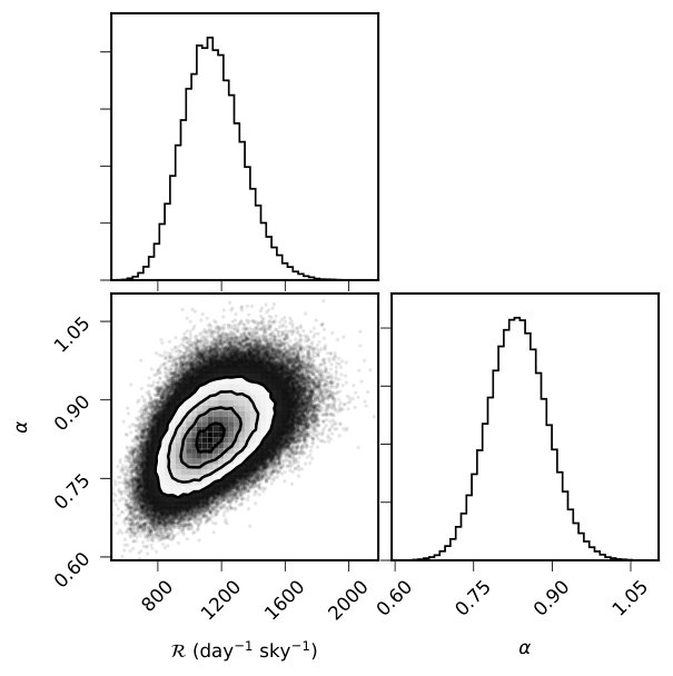
We implement the likelihood formalism of Lawrence et al. 2017 and use Markov Chain Monte Carlo (MCMC) simulation to obtain distributions of $\mathcal{R}_{0}$ and $\alpha$ . We implement the MCMC using the EMCEE⁷⁷ 7 https://github.com/dfm/emcee framework (Foreman-Mackey et al. 2013) with a uniform prior of $\alpha$ and a log-uniform prior on $\mathcal{R}_{0}$ . The resultant posterior distributions for $\log(\mathcal{R}_{0})$ and $\alpha$ are shown in Fig. 6. From this analysis, we infer the FRB rate

\mathcal{R}=1140^{+200}_{-180}\;\left(\frac{S}{\rm Jy}\right)^{-0.83\pm 0.06}\,\text{day}^{-1}\text{sky}^{-1}.

(5)

Here the quoted uncertainties corresponding to 95% confidence intervals. We find a higher rate for the FRBs above 1 Jy, as compared to the Lawrence et al. 2017 which was $587^{+337}_{-315}$ $\text{day}^{-1}\text{sky}^{-1}$ , however, the error regions with both the estimates overlap. Our source count index distribution is shallower than the Lawrence et al. 2017 value of $0.91\pm 0.34$ but lies within their predicted ranges.

Based on this revised event rate, we predict that (for observations exclusively at L-band), GREENBURST will require a further $270^{+65}_{-89}$ days to make its first detection. As can been seen from Table 2, L-Band is in focus for only $\sim$ 65% of the total on sky time. Hence a more realistic estimate for the time to first detection is $365^{+88}_{-120}$ days.

5.3 Detection rate forecasts for other surveys

Table 4: FRB detection rate predictions for various telescopes. From left to right, for each experiment, we list the telescope’s field of view (FOV), the observing bandwidth (

\Delta\nu

), the centre frequency (

F_{\text{centre}}

) and the system equivalent flux density (SEFD) as well as the predicted rate (

R

Telescope	FOV	$\Delta\nu$	$F_{\text{centre}}$	SEFD	$R$
	(deg²)	(MHz)	(MHz)	(Jy)	(day^-1)
CHIME	200	400	600	45	9 $\pm$ 2
HIRAX	56	400	600	6	10 $\pm$ 3
CHORD	130	1200	900	9	4 $\pm$ 1
Northern Cross	350	16	408	95	2 $\pm$ 1

Using our estimates from Eq. 5 we compute expected FRB rates for experiments planned with four telescopes: CHIME (and M. Amiri et al. 2018), CHORD (Vanderlinde et al. 2019), Northern Cross (Locatelli et al. 2020) and HIRAX (Newburgh et al. 2016). To estimate the rate for each survey, we compute the minimum flux density using the radiometer equation assuming a S/N threshold of 10. For experiments at frequencies outside of L-band, we assume a flat spectral index (i.e. no scaling of ${\cal R}$ with frequency). For CHIME and CHORD, the system equivalent flux density

{\rm SEFD}=\frac{T_{\text{rec}}+T_{\text{sky}}}{G},

(6)

where $T_{\text{rec}}$ and $T_{\text{sky}}$ are the receiver and the sky temperatures, respectively, and $G$ is the antenna gain. $T_{\text{sky}}$ is estimated using an average sky temperature of 34 K and a spectral index of –2.6 at a reference frequency of 408 MHz (Haslam et al. 1982). The results from these calculations are shown in Table 4. We also cross-check our results against published detections from the UTMOST telescope, where Caleb et al. 2017 report three FRBs from a 180-day survey. Our prediction for UTMOST over that time period is slightly higher (5 $\pm$ 1 detections) but does not account for the fact that a fraction of the UTMOST survey was conducted at reduced sensitivity (Caleb et al. 2017). Our forecasted rates for the other surveys are very promising and highlight the impact that these surveys will have on future constraints of the all-sky FRB rate.

5.4 Source count index

Our update of the FRB event rate favors a shallower slope $\alpha=0.83$ compared to the expectation from a population of standard candles uniformly distributed in Euclidean space for which $\alpha=1.5$ . These lines are shown in the log $N$ –log $S$ plane in Fig. 7 and are clearly inconsistent with one another. Although detailed analyses of FRB source counts can be found elsewhere (Macquart & Ekers 2017; Macquart & Ekers 2018; James et al. 2019, see, e.g.,), to show what can be learned from future discoveries, it is instructive to place our result in context of two different cosmological models. These are also shown in Fig. 7 and were computed using a simple Monte Carlo simulation in which FRBs were drawn from a population uniformly distributed in comoving volume (green line in the figure) and from a redshift distribution that follows the cosmic star formation history (Madau & Dickinson 2014, see, Eq. 15 of). From the corresponding redshift distributions, luminosity distances were computed for each Monte Carlo sample. In both these cases, the luminosities were assumed to be log–normal in form with a standard deviation (in log space) that is 2% of the mean. The mean luminosity was set somewhat arbitrarily for the purpose of these simulations to be $10^{26}$ W. Flux densities were then computed which resulted in the corresponding cumulative curves.

These models were chosen merely to demonstrate that the impact of these assumptions is to naturally flatten the slope of the source count function from the Euclidean value to something that more closely resembles what is observed. Also shown in these simulations is a steepening of the slopes at higher flux density values. Our analysis in section 5.2 does not account for a possible change in $\alpha$ across the log $N$ –log $S$ plane. In their analysis of Parkes and ASKAP detections, where they considered fluence rather than flux density, James et al. 2019 also found a steepening of the slope at higher fluence values which they suggested could be due to a change in the redshift distribution of the sources. Further analyses of the source count function are definitely required and likely to result in significant insights, particularly from CHIME where a sample of $\sim 700$ FRBs are eagerly anticipated (Fonseca et al. 2020b).

6 Conclusions

In this paper, we present results from the first 156.5 days of commensal FRB searches at the GBT. We use a GPU accelerated single-pulse search pipeline and classify candidates using a deep learning-based algorithm. Our pipeline searches and classifies candidates in real time and logs the relevant telescope metadata using several databases. During our observations, we detected over 2000 single pulses from 20 pulsars which helped to validate our pipeline. We also carried out blind injection analysis of the data and find that we could categorically detect all FRBs with S/N greater than 12.

Our null result is in line with the FRB rate estimates by Bannister et al. 2017. We update the analysis and report a rate of $1140^{+200}_{-180}$ $\text{day}^{-1}\text{sky}^{-1}$ and a shallow source count index of $0.83\pm 0.03$ above a peak flux of 1 Jy. We estimate a further year of observations is required to result in GREENBURST FRB detections. With a stable observing system now in place, we anticipate being able to go well beyond this expectation through continued commensal observing. Our revised FRB rate shows that emerging and ongoing experiments have excellent prospects to discover a very large sample of FRBs in the coming years. Through a Monte Carlo simulation, we show that studies of the source counts of FRBs using this sample will provide significant insights into the luminosity and redshift distributions of FRBs.

Acknowledgements

The Green Bank Observatory is a facility of the National Science Foundation (NSF) operated under cooperative agreement by Associated Universities, Inc. We acknowledge support from the NSF awards AAG-1616042, OIA-1458952 and PHY-1430284.

References

Adamek & Armour (2019) Adamek K., Armour W., 2019, Single Pulse Detection Algorithms for Real-time Fast Radio Burst Searches using GPUs (arXiv:1910.08324)
Agarwal et al. (2019a) Agarwal D., Aggarwal K., Burke-Spolaor S., Lorimer D. R., Garver-Daniels N., 2019a, arXiv e-prints, p. arXiv:1902.06343
Agarwal et al. (2019b) Agarwal D., et al., 2019b, Monthly Notices of the Royal Astronomical Society, 490, 1
Bannister et al. (2017) Bannister K. W., et al., 2017, ApJ, 841, L12
Barsdell et al. (2012) Barsdell B. R., Bailes M., Barnes D. G., Fluke C. J., 2012, Monthly Notices of the Royal Astronomical Society, 422, 379
Bhandari et al. (2017) Bhandari S., et al., 2017, Monthly Notices of the Royal Astronomical Society, 475, 1427
Bhandari et al. (2019) Bhandari S., Bannister K. W., James C. W., Shannon R. M., Flynn C. M., Caleb M., Bunton J. D., 2019, Monthly Notices of the Royal Astronomical Society, 486, 70
Caleb et al. (2017) Caleb M., et al., 2017, Monthly Notices of the Royal Astronomical Society, 468, 3746
Chatterjee et al. (2017) Chatterjee S., et al., 2017, Nature, 541, 58
Chennamangalam et al. (2017a) Chennamangalam J., et al., 2017a, in The Fourteenth Marcel Grossmann Meeting. WORLD SCIENTIFIC, doi:10.1142/9789813226609_0359, https://doi.org/10.1142/9789813226609_0359
Chennamangalam et al. (2017b) Chennamangalam J., et al., 2017b, The Astrophysical Journal Supplement Series, 228, 21
Collaboration et al. (2020) Collaboration T. C., et al., 2020, Periodic activity from a fast radio burst source (arXiv:2001.10275)
Fonseca et al. (2020a) Fonseca E., et al., 2020a, Nine New Repeating Fast Radio Burst Sources from CHIME/FRB (arXiv:2001.03595)
Fonseca et al. (2020b) Fonseca E., et al., 2020b, ApJ, 891, L6
Foreman-Mackey et al. (2013) Foreman-Mackey D., Hogg D. W., Lang D., Goodman J., 2013, PASP, 125, 306
Foster et al. (2017) Foster G., et al., 2017, Monthly Notices of the Royal Astronomical Society, 474, 3847
Golpayegani et al. (2019) Golpayegani G., et al., 2019, Monthly Notices of the Royal Astronomical Society
Haslam et al. (1982) Haslam C. G. T., Salter C. J., Stoffel H., Wilson W. E., 1982, A&AS, 47, 1
James et al. (2019) James C. W., Ekers R. D., Macquart J. P., Bannister K. W., Shannon R. M., 2019, MNRAS, 483, 1342
Karastergiou et al. (2015) Karastergiou A., et al., 2015, MNRAS, 452, 1254
Kumar et al. (2019) Kumar P., et al., 2019, arXiv e-prints, p. arXiv:1908.10026
Law et al. (2018) Law C. J., et al., 2018, The Astrophysical Journal Supplement Series, 236, 8
Lawrence et al. (2017) Lawrence E., Wiel S. V., Law C., Spolaor S. B., Bower G. C., 2017, The Astronomical Journal, 154, 117
Locatelli et al. (2020) Locatelli N. T., et al., 2020, The Northern Cross Fast Radio Burst project. I. Overview and pilot observations at 408 MHz (arXiv:2003.04317)
Lorimer et al. (2000) Lorimer D. R., Kramer M., Müller P., Wex N., Jessner A., Lange C., Wielebinski R., 2000, A&A, 358, 169
Lorimer et al. (2007) Lorimer D. R., Bailes M., McLaughlin M. A., Narkevic D. J., Crawford F., 2007, Science, 318, 777
Macquart & Ekers (2017) Macquart J.-P., Ekers R. D., 2017, Monthly Notices of the Royal Astronomical Society, 474, 1900
Macquart & Ekers (2018) Macquart J. P., Ekers R., 2018, MNRAS, 480, 4211
Macquart et al. (2010) Macquart J.-P., et al., 2010, Publications of the Astronomical Society of Australia, 27, 272
Madau & Dickinson (2014) Madau P., Dickinson M., 2014, Annual Review of Astronomy and Astrophysics, 52, 415
Madison et al. (2019) Madison D. R., et al., 2019, The Astrophysical Journal, 887, 252
Magro et al. (2011) Magro A., Karastergiou A., Salvini S., Mort B., Dulwich F., Adami K. Z., 2011, Monthly Notices of the Royal Astronomical Society, 417, 2642
Manchester et al. (2005) Manchester R. N., Hobbs G. B., Teoh A., Hobbs M., 2005, The Astronomical Journal, 129, 1993
Men et al. (2019) Men Y., et al., 2019, Monthly Notices of the Royal Astronomical Society
Newburgh et al. (2016) Newburgh L. B., et al., 2016, in Hall H. J., Gilmozzi R., Marshall H. K., eds, Ground-based and Airborne Telescopes VI. SPIE, doi:10.1117/12.2234286, https://doi.org/10.1117/12.2234286
Osłowski et al. (2019) Osłowski S., et al., 2019, Monthly Notices of the Royal Astronomical Society, 488, 868
Petroff et al. (2016) Petroff E., et al., 2016, Publ. Astron. Soc. Australia, 33, e045
Petroff et al. (2018) Petroff E., et al., 2018, Monthly Notices of the Royal Astronomical Society
Qiu et al. (2019) Qiu H., Bannister K. W., Shannon R. M., Murphy T., Bhandari S., Agarwal D., Lorimer D. R., Bunton J. D., 2019, Monthly Notices of the Royal Astronomical Society, 486, 166
Rajwade et al. (2020) Rajwade K. M., et al., 2020, arXiv e-prints, p. arXiv:2003.03596
Sammut & Webb (2017) Sammut C., Webb G. I., eds, 2017, Encyclopedia of Machine Learning and Data Mining. Springer US, doi:10.1007/978-1-4899-7687-1, https://doi.org/10.1007/978-1-4899-7687-1
Shannon et al. (2018) Shannon R. M., et al., 2018, Nature, 562, 386
Spitler et al. (2014) Spitler L. G., et al., 2014, The Astrophysical Journal, 790, 101
Surnis et al. (2019) Surnis M. P., et al., 2019, Publ. Astron. Soc. Australia, 36, e032
The CHIME/FRB Collaboration et al. (2019a) The CHIME/FRB Collaboration et al., 2019a, arXiv e-prints,
The CHIME/FRB Collaboration et al. (2019b) The CHIME/FRB Collaboration et al., 2019b, arXiv e-prints, p. arXiv:1908.03507
Thornton et al. (2013) Thornton D., et al., 2013, Science, 341, 53
Vanderlinde et al. (2019) Vanderlinde K., et al., 2019, LRP 2020 Whitepaper: The Canadian Hydrogen Observatory and Radio-transient Detector (CHORD) (arXiv:1911.01777)
Zhang et al. (2019) Zhang S.-B., Hobbs G., Dai S., Toomey L., Staveley-Smith L., Russell C. J., Wu X.-F., 2019, Monthly Notices of the Royal Astronomical Society: Letters, 484, L147
and M. Amiri et al. (2018) and M. Amiri et al., 2018, The Astrophysical Journal, 863, 48