Unstructured Space-Time Finite Element Methods for Optimal Sparse
Control of
Parabolic EquationsThis work has been supported by Johann Radon Institute for
Computational and Applied Mathematics (RICAM) during the special semester on
optimization that took place between 14th October and 11th December,
2019, at RICAM in Linz, Austria.
Abstract
We consider a space-time finite element method on fully unstructured simplicial meshes for optimal sparse control of semilinear parabolic equations. The objective is a combination of a standard quadratic tracking-type functional including a Tikhonov regularization term and of the -norm of the control that accounts for its spatio-temporal sparsity. We use a space-time Petrov-Galerkin finite element discretization for the first-order necessary optimality system of the associated discrete optimal sparse control problem. The discretization is based on a variational formulation that employs piecewise linear finite elements simultaneously in space and time. Finally, the discrete nonlinear optimality system that consists of coupled forward-backward state and adjoint state equations is solved by a semismooth Newton method.
Keywords: space-time finite element method, optimal sparse control,
semilinear parabolic equations
MSC 2010: 49J20, 35K20, 65M60, 65M50, 65M15, 65Y05
1 Introduction
Optimal sparse control with the -norm of the control in the objective functional and with linear elliptic state equations has been analyzed in [30] about a decade ago. The method was extended to semilinear elliptic optimal control problems in [10] and to problems governed by elliptic equations with uncertain coefficients in [27]. In [15, 16, 29], the authors investigated problems of optimal sparse control for the Schlögl and FitzHugh-Nagumo systems, where traveling wave fronts or spiral waves were controlled. Directionally spatio-temporal optimal sparse control of linear/semilinear elliptic/parabolic equations and its corresponding optimality conditions was studied in [11, 20]. Optimality conditions for directionally sparse parabolic control problems without control constraints were considered in [13]; see also [14]. The optimal sparse controls considered therein exhibit sparsity in space, but not necessarily in time. We also mention another class of optimal sparse control problems for parabolic equations with controls in measure spaces instead of -spaces, see, e.g., [5, 8, 12, 17, 23]. A thorough review of the existing literature on this challenging topic is beyond the scope of this work. Therefore, we refer to the recent survey article [7] on sparse solutions in optimal control of both elliptic and parabolic equations and the references therein.
Moreover, numerical approximations of optimal sparse controls of elliptic and parabolic problems were of great interest. For example, the standard -point stencil was used in [30] for the discretization of elliptic optimal sparse control problems. In [10], the authors proved rigorous error estimates for the finite element approximation of semilinear elliptic sparse control problems with with box constraints on the control. In the discrete optimality conditions, they used piecewise linear approximations for the state and adjoint state, while a piecewise constant ansatz was applied to the control and the subdifferential. We also mention the approximation of sparse controls by piecewise linear functions in [9]. Here, the authors adopt special quadrature formulae to discretize the squared -norm and the -norm of the control in the objective functional. This leads to an elementwise representation of the control and of the subdifferential.
Later, error estimates were derived for the space-time finite element approximation of parabolic optimal sparse control problems without control constraints in [13]. The discretization was performed on tensor-structured space-time meshes. In the associated discrete optimal control problem, these authors used a spatio-temporal finite element ansatz for the state that consists of products of continuous, piecewise linear basis functions in space, and piecewise constant basis functions in time. For the control, they utilize space-time elementwise constant basis functions. The same space as for the state was employed for the adjoint state in the discrete optimality system. Improved approximation rates were achieved in [14]. For the control discretization, they employ basis functions that are continuous and piecewise linear in space and piecewise constant in time. These methods can be re-interpreted as an implicit Euler discretization of the spatially discretized optimality system.
For optimal sparse control of the Schlögl and FitzHugh-Nagumo models that were considered in [15], a semi-implicit Euler-method in time and continuous piecewise linear finite elements in space were applied to both the state and adjoint state equations. Recently, in [38], for the optimal control of the convective FitzHugh-Nagumo equation, the state and adjoint state equations were discretized by a symmetric interior penalty Galerkin method in space and the backward Euler method in time.
In contrast to the discretization methods discussed above, we apply continuous space-time finite element approximations on fully unstructured simplicial meshes for parabolic optimal sparse control problems with control constraints. This can be seen as an extension of the Petrov-Galerkin space-time finite element method proposed in [32] for parabolic problems, and in our recent work [25] for parabolic optimal control problems. This kind of unstructured space-time finite element approaches has gained increasing interest; see, e.g., [2, 3, 22, 24, 34, 36, 39], and the survey article [35].
In comparison to the more conventional time-stepping methods or tensor-structured space-time methods [18, 19, 28], this unstructured space-time approach provides us with more flexibility in constructing parallel space-time solvers such as parallel space-time algebraic multigrid preconditioners [24] or space-time balancing domain decomposition by constraints (BDDC) preconditioners [26]. Moreover, it becomes more convenient to realize simultaneous space-time adaptivity on unstructured space-time meshes [24, 25, 33] than the other methods. Here, time is just considered as another spatial coordinate. For more comparisons of our space-time finite element methods with others, we refer to [35].
The remainder of this paper will be structured as follows: Section 2 describes a model optimal sparse control problem that we aim to solve. Some preliminary existing results concerning optimality conditions are given in Section 3. The space-time finite element discretization of the associated discrete optimal control problem, the resulting discrete optimality conditions, as well as the application of the semismooth Newton iteration are discussed in Section 4. The applicability of our proposed method is confirmed by two numerical examples in Section 5. Finally, some conclusions are drawn in Section 6.
2 The optimal sparse control model problem
We consider the optimal sparse control problem
| (1) |
where the admissible set is
| (2) |
and is the unique solution of the state equation
| (3) | ||||||
Here, the spatial computational domain , , is supposed to be bounded and Lipschitz, is the fixed terminal time, denotes the partial time derivative, the spatial Laplacian, and the source term acts as a distributed control in . Moreover, is a given desired state. We further assume
The nonlinear reaction term is defined by
with given real numbers . The functional defined by is Lipschitz continuous and convex but not Fréchet differentiable. We notice that similar model problems for semilinear equations have been studied, e.g., in [7, 11].
3 Preliminary results
Let us recall some facts that are known from literature, e.g., [7]. For all , , the state equation (3) has a unique solution , where
| (4) |
Here, . The mapping is continuously Fréchet differentiable in these spaces. The optimal control problem has at least one optimal control that is denoted by ; the associated optimal state is denoted by .
If is a locally optimal control of the model problem, then there exist a unique adjoint state and some such that solves the optimality system
| (5a) | ||||
| (5b) | ||||
| (5c) | ||||
where . A detailed discussion of this optimality system leads to the relations
| (6a) | |||
| (6b) | |||
| (6c) | |||
that hold for a.a. ; see, e.g., [15]. Here, the projection is defined by ; see, e.g., [37]. The subdifferential of the -norm of the control is given as follows:
for a.a. and . By these relations, we obtain the following form of an optimal control:
| (7) |
The set accounts for the sparsity of the control.
Eliminating the control from the optimality system and using the projection formulae above, we obtain the following system for the state and the adjoint state:
| (8a) | ||||
| (8b) | ||||
Let us define the Bochner spaces for the state and adjoint state variables as follows:
Our space-time variational formulation for the coupled system (8) reads: Find and such that the variational equations
| (9a) | |||
| (9b) | |||
hold for all . This system is solvable, because the optimal control problem has at least one solution. Due to the projection formula on the right hand side of (9a), we need special care to discretize the optimality system. In fact, following the discretization scheme proposed in [1], we go back to the variational inequality (5c) and use piecewise constant approximation for the control in order to derive first order necessary optimality conditions for the associated discrete optimal control problem. We will discuss this in the forthcoming Section.
4 Space-time finite element discretization
For the space-time finite element approximation of the optimal control problem (1), we consider an admissible triangulation of the space-time domain into shape regular simplicial finite elements . Here, the mesh size is defined by with being the diameter of the element ; see, e.g., [6, 31]. For simplicity, we assume to be a polygonal spatial domain. Therefore, the triangulation exactly covers .
Let be the space of continuous and piecewise linear functions that are defined with respect to the triangulation . The discrete variational form of the state equation (3) reads as follows: Find such that
| (10) |
is satisfied for all . For approximating the control , we define the space
An element can be represented in the form
with being the characteristic function of . Moreover, the set of discrete admissible controls is defined by
Now, we consider the discrete optimal control problem
where denotes the solution of the discrete variational problem (10) with the discrete control . We assume that the discrete optimal control problem has at least one locally optimal control that is denoted by . The associated state is denoted by . If is a locally optimal control of the discrete optimal control problem, then there exists a unique adjoint state and such that solves the discrete optimality system
| (11a) | |||
| (11b) | |||
| (11c) | |||
The existence of a solution to the discretized optimality system will not be discussed in this paper. We tacitly assume that a locally unique solution exists. Note that is equivalent to the form
Then, the inequality (11c) can be represented as follows:
which is recasted in the equivalent form
for all . Therefore, we have the projection representation formula [37]
| (12) |
for the optimal control on each element . From this, we have the following results:
The above results are obtained by the discretization approach proposed in [1, 10] for the optimal control of semilinear elliptic equations, and in [15] of the Schlögl and FitzHugh-Nagumo systems. In fact, by a close look to the projection formula, we have the following form of the discrete optimal control:
| (13) |
where
Inserting (12) into (11a), we obtain an equivalent form of the discrete optimality system that consists of the state and adjoint state equations. Namely, find and such that solves the coupled system
| (14a) | |||
| (14b) | |||
The convergence of the solution of the discrete optimal control problem to the solution of its associated continuous optimal control problem as well as the error analysis of our finite element approximation are beyond the scope of this work and will be studied elsewhere.
To solve the above discrete coupled nonlinear optimality system, we apply the semismooth Newton method as discussed in [30], where a generalized derivative needs to be computed at each Newton iteration. In fact, each iteration turns out to be one step of a primal-dual active set strategy [21]: Given , find such that
and
are fulfilled, and , with some damping parameter .
5 Numerical experiments
For the two numerical examples considered in this section, we set , , and therefore . Using an octasection-based refinement [4], we uniformly decompose the space-time cylinder until the mesh size reaches . Therefore, the total number of degrees of freedom for the coupled state and adjoint state equations is . We will also use an adaptive refinement procedure that is driven by a residual based error indicator for the coupled state and adjoint state system similar to that one that was developed for the state equation in [33]. We perform our numerical tests on a desktop with Intel@ Xeon@ Processor E5-1650 v4 ( MB Cache, GHz), and GB memory. For the nonlinear first order necessary optimality system, we use the relative residual error as a stopping criterion in the semismooth Newton iteration, whereas the algebraic multigrid preconditioned GMRES solver for the linearized system at each Newton iteration is stopped after a residual error reduction by ; cf. also [35].
5.1 Moving target (Example 1)
In the first example, the desired state is given by the function
which is adapted from an example constructed in [11]; see an illustration of the target at time , , and in Fig. 1. The same desired state was also used in the numerical test for spatially directional sparse control in [13, 14]. The parameters in the optimal control problem are , , , and . For the nonlinear reaction term in the state equation, we set . Homogeneous initial and Dirichlet boundary conditions are used for the state equation.


To reach the relative residual error for the nonlinear first order necessary optimality system, we needed and semismooth Newton iterations for the nonsparse and sparse optimal control, respectively; see Fig.2. We clearly see a superlinear convergence of the semismooth Newton method. The total system assembling and solving time is about and hours on the desktop computer, respectively.

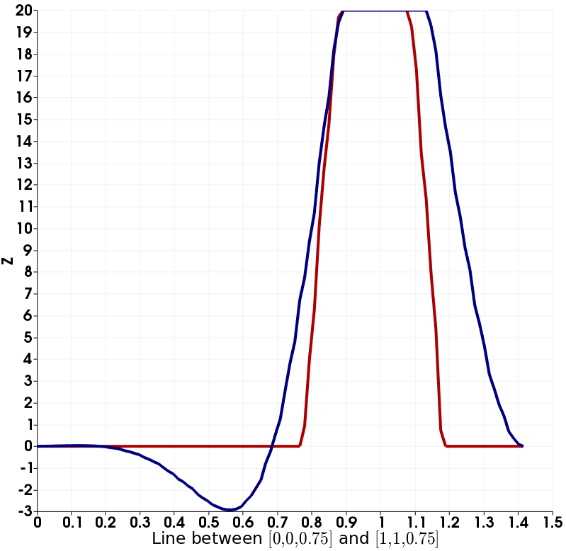
Comparisons of sparse and nonsparse controls as well as of associated states at different times are displayed in Fig. 3 and Fig. 4, respectively. A close look to sparse and nonsparse controls along different lines in the space-time domain is illustrated in Fig. 5. In this example, we clearly see that the cost functional promotes spatial and temporal sparsity, with some precision loss of the associated state to the target, cf. Fig. 4.


5.2 Turning wave target (Example 2)
In this example, we consider the target
where . This is an adapted version of the turning wave example considered in [15]. The wave front turns degrees from time to , and remains fixed after ; see the target at , , , and as illustrated in Fig. 6.


The nonlinear reaction term is given by . We use the initial data
on , and homogeneous Neumann boundary condition on for the state. As parameters, we use , for the sparse case and , for the nonsparse case. The bounds and are set for both cases.
To solve the nonlinear first order necessary optimality system, we needed and semismooth Newton iterations for the nonsparse and sparse optimal control, respectively; see Fig. 7. The total system assembling and solving time is about and hours on the desktop computer, respectively.

The numerical solutions of sparse and nonsparse controls as well as associated optimal states are illustrated in Fig. 8. We clearly see certain sparsity of our optimal sparse control as compared to pure -regularization, without too much precision loss of the associated state to the target. A closer look to the sparse and nonsparse controls confirms that our optimal sparse control exhibits sparsity with respect to the spatial direction; see Fig. 9.


Instead of an uniform refinement, we may also adopt an adaptive strategy. In this way, local refinements are made in the region where the solution shows a more local character, whereas coarser meshes appear in the other region. For example, in the optimal sparse control case (, ), we start from an initial mesh with grid points, in each spatial and the temporal direction. We use a residual based error indicator for the coupled state and adjoint state system to guide our adaptive mesh refinement, similar to the approach [33]. After the th adaptive octasection refinement [4], the mesh contains grid points; see the adaptive space-time mesh and the meshes on the cutting plans at different times in Fig. 10. As we observe, the adaptive refinements follow the rotation of the wave front of the state.


6 Conclusions
In this work, we have considered a space-time Petrov-Galerkin finite element method on fully unstructured simplicial meshes for semilinear parabolic optimal sparse control problems. The objective functional involves the well-known -norm of the control in addition to the standard -regularization term. The proposed method is able to capture spatio-temporal sparsity, which has been confirmed by our numerical experiments. A rigorous convergence and error analysis of our space-time Petrov-Galerkin finite element methods for such optimal sparse control problems is left for future work.
References
- [1] N. Arada, E. Casas, and F. Tröltzsch. Error estimates for the numerical approximation of a semilinear elliptic control problem. Comput. Optim. Appl., 23:201–229, 2002.
- [2] R. E. Bank, P. S. Vassilevski, and L. T. Zikatanov. Arbitrary dimension convection-diffusion schemes for space-time discretizations. J. Comput. Appl. Math., 310:19–31, 2017.
- [3] M. Behr. Simplex space-time meshes in finite element simulations. Int. J. Numer. Meth. Fluids, 57:1421–1434, 2008.
- [4] J. Bey. Tetrahedral grid refinement. Computing, 55:355–378, 1995.
- [5] A. C. Boulanger and P. Trautmann. Sparse optimal control of the KdV-Burgers equation on a bounded domain. SIAM J. Control Optim., 55(6):3673–3706, 2017.
- [6] D. Braess. Finite Elements: Theory, Fast Solvers, and Applications in Solid Mechanics. Cambridge University Press, 2007.
- [7] E. Casas. A review on sparse solutions in optimal control of partial differential equations. SeMA, 74:319–344, 2017.
- [8] E. Casas, C. Clason, and K. Kunisch. Parabolic control problems in measure spaces with sparse solutions. SIAM J. Control Optim., 51(1):28–63, 2013.
- [9] E. Casas, R. Herzog, and G. Wachsmuth. Approximation of sparse controls in semilinear equations by piecewise linear functions. Numer. Math., 122:645–669, 2012.
- [10] E. Casas, R. Herzog, and G. Wachsmuth. Optimality conditions and error analysis of semilinear elliptic control problems with cost functional. SIAM J. Optim., 22(3):795–820, 2012.
- [11] E. Casas, R. Herzog, and G. Wachsmuth. Analysis of spatio-temporally sparse optimal control problems of semilinear parabolic equations. ESAIM: COCV, 23(1):263–295, 2017.
- [12] E. Casas and K. Kunisch. Parabolic control problems in space-time measure spaces. ESAIM: COCV, 22(2):355–370, 2016.
- [13] E. Casas, M. Mateos, and A. Rösch. Finite element approximation of sparse parabolic control problems. Math. Control Relat. Fields, 7(3):393–417, 2017.
- [14] E. Casas, M. Mateos, and A. Rösch. Improved approximation rates for a parabolic control problem with an objective promoting directional sparsity. Comput. Optim. Appl., 70:239–266, 2018.
- [15] E. Casas, C. Ryll, and F. Tröltzsch. Sparse optimal control of the Schlögl and FitzHugh-Nagumo systems. Comput. Methods Appl. Math., 13(4):415–442, 2013.
- [16] E. Casas, C. Ryll, and F. Tröltzsch. Second order and stability analysis for optimal sparse control of the FitzHugh-Nagumo equation. SIAM J. Control and Optim., 53(4):2168–2202, 2015.
- [17] E. Casas and E. Zuazua. Spike controls for elliptic and parabolic PDEs. Syst. Control Lett., 62(4):311–318, 2013.
- [18] M. J. Gander. 50 years of time parallel integration. In Thomas Carraro, Michael Geiger, Stefan Körkel, and Rolf Rannacher, editors, Multiple Shooting and Time Domain Decomposition, pages 69–114. Springer Verlag, Heidelberg, Berlin, Cham, 2015.
- [19] M. J. Gander and M. Neumüller. Analysis of a new space-time parallel multigrid algorithm for parabolic problems. SIAM J. Sci. Comput., 38(4):A2173–A2208, 2016.
- [20] R. Herzog, G. Stadler, and G. Wachsmuth. Directional sparsity in optimal control of partial differential equations. SIAM J. Control Optim., 50(2):943–963, 2012.
- [21] K. Ito and K. Kunisch. Lagrange multiplier approach to variational problems and applications, volume 15 of Advances in Design and Control. Society for Industrial and Applied Mathematics (SIAM), Philadelphia, PA, 2008.
- [22] V. Karyofylli, L. Wendling, M. Make, N. Hosters, and M. Behr. Simplex space-time meshes in thermally coupled two-phase flow simulations of mold filling. Compur. Fluids, 192:104261, 2019.
- [23] K. Kunisch, K. Pieper, and B. Vexler. Measure valued directional sparsity for parabolic optimal control problems. SIAM J. Control Optim., 52(5):3078–3108, 2014.
- [24] U. Langer, Neumüller M., and Schafelner A. Space-time finite element methods for parabolic evolution problems with variable coefficients. In T. Apel, U. Langer, A. Meyer, and O. Steinbach, editors, Advanced Finite Element Methods with Applications: Selected Papers from the 30th Chemnitz Finite Element Symposium 2017, pages 247–275, Cham, 2019. Springer International Publishing.
- [25] U. Langer, O. Steinbach, F. Tröltzsch, and H. Yang. Unstructured space-time finite element methods for optimal control of parabolic equations. In preparation, 2020.
- [26] U. Langer and H. Yang. BDDC preconditioners for a space-time finite element discretization of parabolic problems. In Domain Decomposition Methods in Science and Engineering XXV, Cham, 2020. Springer International Publishing. To appear.
- [27] C. Li and G. Stadler. Sparse solutions in optimal control of PDEs with uncertain parameters: The linear case. SIAM J. Control Optim., 57(1):633–658, 2019.
- [28] A. Nägel, D. Logashenko, J. B. Schroder, and U. M. Yang. Aspects of solvers for large-scale coupled problems in porous media. Transp. Porous. Med., 130:363–390, 2019.
- [29] C. Ryll, J. Löber, S. Martens, H. Engel, and F. Tröltzsch. Analytical, optimal, and sparse optimal control of traveling wave solutions to reaction-diffusion systems. In E. Schöll, S. H. L. Klapp, and P. Hövel, editors, Control of Self-Organizing Nonlinear Systems, pages 189–210. Springer International Publishing, Cham, 2016.
- [30] G. Stadler. Elliptic optimal control problems with -control cost and applications for the placement of control devices. Comput. Optim. Appl., 44:159–181, 2009.
- [31] O. Steinbach. Numerical Approximation Methods for Elliptic Boundary Value Problems. Springer-Verlag New York, 2008.
- [32] O. Steinbach. Space-time finite element methods for parabolic problems. Comput. Methods Appl. Math., 15:551–566, 2015.
- [33] O. Steinbach and H. Yang. Comparison of algebraic multigrid methods for an adaptive space-time finite-element discretization of the heat equation in 3d and 4d. Numer. Linear Algebra Appl., 25(3):e2143, 2018.
- [34] O. Steinbach and H. Yang. A space-time finite element method for the linear bidomain equations. In T. Apel, U. Langer, A. Meyer, and O. Steinbach, editors, Advanced Finite Element Methods with Applications: Selected Papers from the 30th Chemnitz Finite Element Symposium 2017, pages 323–339, Cham, 2019. Springer International Publishing.
- [35] O. Steinbach and H. Yang. Space-time finite element methods for parabolic evolution equations: discretization, a posteriori error estimation, adaptivity and solution. In O. Steinbach and U. Langer, editors, Space-Time Methods: Application to Partial Differential Equations, Radon Series on Computational and Applied Mathematics, pages 207–248, Berlin, 2019. de Gruyter.
- [36] I. Toulopoulos. Space-time finite element methods stabilized using bubble function spaces. Appl. Anal., 0(0):1–18, 2018.
- [37] F. Tröltzsch. Optimal control of partial differential equations: Theory, methods and applications, volume 112 of Graduate Studies in Mathematics. American Mathematical Society, Providence, Rhode Island, 2010.
- [38] M. Uzunca, T. Küçükseyhan, H. Yücel, and B. Karasözen. Optimal control of convective Fitzhugh-Nagumo equation. Comput. Math. Appl., 73(9):2151–2169, 2017.
- [39] M. von Danwitz, V. Karyofylli, N. Hosters, and M. Behr. Simplex space-time meshes in compressible flow simulations. Int. J. Numer. Meth. Fluids, 91(1):29–48, 2019.