Thermodynamic cost, speed, fluctuations, and error reduction of biological copy machines
Abstract
Due to large fluctuations in cellular environments, transfer of information in biological processes without regulation is inherently error-prone. The mechanistic details of error-reducing mechanisms in biological copying processes have been a subject of active research; however, how error reduction of a process is balanced with its thermodynamic cost and dynamical properties remain largely unexplored. Here, we study the error reducing strategies in light of the recently discovered thermodynamic uncertainty relation (TUR) that sets a physical bound to the cost-precision trade-off relevant in general dissipative processes. We found that the two representative copying processes, DNA replication by the exonuclease-deficient T7 DNA polymerase and mRNA translation by the E. coli ribosome, reduce the error rates to biologically acceptable levels while also optimizing the processes close to the physical limit dictated by TUR.
Biological copying processes, which include DNA replication, transcription, and translation, have evolved error-reducing mechanisms to faithfully transmit information in the genetic code. In their seminal papers in the 1970s, Hopfield and Ninio Hopfield 1974; Ninio 1975 proposed the kinetic proofreading mechanism to show that the energy-burning action of the mechanism can reduce the error rate. Shortly after, Bennett showed that the difference between kinetic barriers involving the incorporation of correct and incorrect substrates could be capitalized on to reduce the error rate under nonequilibrium chemical driving forces Bennett 1976. Despite differences in their mechanistic details, both models share a common feature that the reduction of copying error incurs free energy cost. Since these pioneering works, there have been a number of studies devoted to understanding the relation between the error reduction, speed, and energy consumption not only in the biological copying processes Banerjee et al. 2017a; Cady and Qian 2009; Mallory et al. 2019; Mellenius and Ehrenberg 2017; Murugan et al. 2012; Rao and Peliti 2015, but also in more general biochemical networks, including those related to sensory adaptation, circadian rhythm, and metabolic control Cao et al. 2015; Hartich et al. 2015; François and Altan-Bonnet 2016; Lan and Tu 2013; Marsland et al. 2019; Qian and Beard 2006.
Besides the faithful transmission of genetic information, the primary goal of biological copying processes is to generate biomass in the forms of DNA, RNA, and proteins. Intuitively, however, error reduction comes at the cost of energy dissipation or slowing down of the process. Furthermore, fluctuations in biomass synthesis, which concomitantly increase with heat dissipation for Michaelis-Menten type processes Hwang and Hyeon 2017, also have to be suppressed below a biologically acceptable level. For instance, DNA replication in early fly embryogenesis occurs at high speed with exquisite precision; a modest change of 10 % in replication timing could be lethal Djabrayan et al. 2019. Similarly, for translation, it is well known that cells must express genes at the right protein copy number for optimal function in a given environment Dekel and Alon 2005; Scott et al. 2014; Li et al. 2014; regulatory mechanisms are developed to suppress the copy number fluctuation in gene expression Fraser et al. 2004. How biological processes balance these conflicting requirements is a fundamental subject to explore. To address such an issue, the recently developed thermodynamic uncertainty relation (TUR) Barato and Seifert 2015, which offers a quantitative bound for dissipative processes at nonequilibrium steady states (NESS), is well suited.
TUR expresses the trade-off between the thermodynamic cost and uncertainty of dynamical processes in NESS and specifies its physical bound as follows:
| (1) |
This form of TUR holds for most of biological processes that can be represented either by stochastic jump processes on a kinetic network or by overdamped Langevin dynamics Gingrich et al. 2016; Hyeon and Hwang 2017; Dechant and Sasa 2018a; Pigolotti et al. 2017, though extensions to more general conditions, which adjust the lower bound of the original relation, have also been discussed in recent years Lee et al. 2018; Horowitz and Gingrich 2017; Brandner et al. 2018; Barato et al. 2018; Chun et al. 2019; Marsland et al. 2019; Hasegawa and Van Vu 2019; Timpanaro et al. 2019; Horowitz and Gingrich 2019. Briefly, is a relative uncertainty (or error) in an output observable best representing the dynamic process at time , and denotes the thermodynamic cost or heat dissipation in generating the dynamic trajectory. The inequality in Eq.1 allows one to quantitatively assess the physical limit to the precision that a dynamical process can maximize for a given amount of dissipation. Recently, , which is bounded between 0 and 1, was used to quantify the “transport efficiency” of molecular motors Dechant and Sasa 2018a. When is written in the form of with and being the diffusivity and velocity of a molecular motor, the motor characterized with a small can be interpreted as an efficient cargo transporter, because it transports cargos with high velocity (), small fluctuation (), but with small dissipation rate () Hwang and Hyeon 2018. Biosynthetic reactions that are efficient in suppressing fluctuations in product formation can also be characterized by small .
This work is organized into four parts. (i) We first introduce the basics of biological copying processes by reviewing the two distinct error reducing strategies by Bennett Bennett 1976 and Hopfield Hopfield 1974. (ii) We evaluate the error rate and of the replication process by the exonuclease-deficient T7 DNA polymerase, a model process reminiscent of the kinetic discrimination mechanism by Bennett. (iii) We analyze a model of mRNA translation where both Bennett’s kinetic discrimination and Hopfield’s kinetic proofreading are employed to lower the error rate, and calculate for translating a codon into a polypeptide chain. (vi) Lastly, we consider a more realistic model of mRNA translation that explicitly accounts for 42 types of aa-tRNA, and show that kinetic proofreading can suppress the fluctuation in the rate of polypeptide production.
I Results
Error reducing mechanisms by Bennett and Hopfield. We briefly describe the two representative error reducing mechanisms, one by Bennett and the other by Hopfield. In a nutshell, the essence of the two mechanisms lies in an energy-dissipating enzymatic reaction of copy machines comprised of multiple kinetic cycles that can discriminate correct substrates from incorrect ones. Illustrated in Fig.1A is an exemplary biological copying process where information of DNA sequence is copied by the DNA polymerase.
When the average reaction currents along the kinetic path associated with correct and incorrect substrate incorporation to the copy strand are defined as and , respectively, the error probability, which will be discussed throughout this paper, is given by the ratio of two reaction currents
| (2) |
Error reducing strategies of biological copying processes are at work to minimize to a level acceptable for the survival of an organism.

The mechanism of Bennett model (Fig.1) Bennett 1976 uses the chemical potential of substrates, whose concentrations are kept out of equilibrium (), as the free energy drive. In the model, correct and incorrect substrates are kinetically discriminated with different kinetic barriers, but with no difference in binding stabilities of the two substrate types. At equilibrium, , and the error rate () is solely determined by the ratio of equilibrium binding probabilities to copying system (), so that . When the free energy drive is large (), the error rate converges to , which is solely determined by the difference between the kinetic barriers for substrate binding, . Thus, as long as , the mechanism can reduce the value of from to at the expense of the free energy drive. See SI Text for the generalization of Bennett model where the equilibrium error rate is given by .
Meanwhile, the original Hopfield model Hopfield 1974 (see Fig.1B) assumes that the binding rates ( or in Fig.1B) for the correct and incorrect substrates are identical (). In discriminating correct substrates from incorrect ones, the mechanism takes advantage of the facilitated unbinding of incorrect substrate from the copying system twice along the reaction path ( and in Fig.1B, bottom), assisted by the extra free energy from molecular fuel consumption (GTP or ATP hydrolysis), which renders the reaction paths and effectively irreversible. The substrates complementary to the template polymer sequence are more likely to be polymerized, whereas the preferential unbinding of incorrect substrates from the copying complex end up with expending the energy for proofreading, giving rise to the futile cycle. The mechanism of Hopfield model, called the kinetic proofreading mechanism, reduces the error rate from down to Hopfield 1974.
Real biological copying processes modify or combine the above two error-reducing strategies.
More details on the different types of error reducing strategies and their combined effects can be found in refs. Sartori and Pigolotti 2013; Pigolotti and Sartori 2016.
Kinetic discrimination of dNTP by the T7 DNA polymerase. The DNA polymerase, in the absence of exonuclease activity, is an enzyme that adapts the kinetic discrimination mechanism to reduce errors in replication Tsai and Johnson 2006; Johnson 2010; Cady and Qian 2009. In its simplest form, the replication dynamics of DNA polymerases can be represented by a double-cyclic reversible 3-state network consisting of two topologically identical subcycles for the incorporation of correct and incorrect nucleotides (Fig.2A). Following the binding of the substrate (dNTP) (), the polymerase on DNA undergoes conformational change (). Finally, the effectively irreversible polymerization associated with dNTP incorporation () with and , completes the kinetic cycle. The free energy difference between the binding of correct and incorrect nucleotides is approximately Goodman 1997, which implies that the error probability at equilibrium is . In the presence of non-equilibrium drive, the conditions of and , engendering much larger reaction current along than that along , allows DNA polymerases to reduce below Tsai and Johnson 2006; Johnson 2010.

As the total reaction current of polymerization, , is a natural output observable accessible, for instance, in single molecule experiments Abbondanzieri et al. 2005; Wen et al. 2008; Kaiser et al. 2011, we calculate of DNA replication as (see Eq.1, and Materials and Methods)
| (3) |
Alternatively, one could conceive choosing the current of correct sequence incorporation, , as the output variable; however, unlike that of , the measurement of requires the explicit knowledge of the DNA sequence being synthesized, which is not readily accessible to an experimental observer. As long as is small, it is expected that , and ; thus, choosing as the output variable instead of will not significantly alter the value of .
The free energy cost for a single step of polymerization (affinity, ) can be written as
| (4) |
where and are the chemical potential difference along the correct and incorrect and polymerization cycles, respectively. can be decomposed into the free energy gain () and the Shannon-entropy () arising from the chance of incorporating correct versus incorrect monomers in the copy strand. It is noteworthy that although is usually small compared to , it represents a fundamental thermodynamic property associated with stochastic copying processes (see Eq. S21) Sartori and Pigolotti 2015.
We explore how is affected when dNTP concentration ([dNTP]), which serves as a proxy for the chemical potential drive ( in Eq. S10), increases. We assume that the four types of dNTPs (A, G, C, T) are maintained in solution at equal concentrations, and use experimentally determined kinetic rates of the exonuclease-deficient T7 DNA polymerase to calculate and (see Table S1) Tsai and Johnson 2006. With increasing [dNTP], the reaction current flows predominantly in one of the subcycles (), and decreases monotonically to values consistent with experimental measurements Cady and Qian 2009; Kunkel et al. 1994 (Fig. 2B); by contrast, displays non-monotonic variation (Fig. 2C). For , two minima are identified, one at , and the other at ( M), suggesting a complex interplay between the dissipation, current and its fluctuation. The suboptimal value of with respect to substrate concentration was also observed in models of transport motors Hwang and Hyeon 2018. Notably, the latter minimum is found near the range of the in vivo [dNTP] in E. coli ( M Bochner and Ames 1982; Buckstein et al. 2008; Schaaper and Mathews 2013) (Fig. 2C).

To understand the nature of the two minima of , we calculated of an analogously defined unicyclic 3-state model with kinetic rates identical to those of the correct nucleotide incorporation cycle.
The comparison between the of the two models suggests:
(i) the global minimum is formed near the DB condition
;
(ii) the other minimum at M arises from the Michaelis-Menten (MM) type enzyme kinetics.
For Michaelis-Menten enzyme reactions, is suboptimized when the substrate concentration is near the Michaelis-Menten constant (), where the response of the reaction is maximal with respect to the logarithmic variation of substrate concentration (see SI text).
Simplified model of mRNA translation. Since its introduction by Hopfield and Ninio Hopfield 1974; Ninio 1975, kinetic proofreading has been the most extensively discussed error reducing strategy Banerjee et al. 2017a; Murugan et al. 2012; Rao and Peliti 2015; Pigolotti and Sartori 2016. The proofreading reduces copy error by a resetting reaction that incurs an extra free energy. We study the effect of kinetic proofreading on by taking mRNA translation of the E. coli ribosome as our model system (see Fig. 3).
The ribosome translates mRNA sequences into a polypeptide by reading codons, each consisting of three consecutive nucleic acids (Fig. 3A). When an aa-tRNA of a ‘matching’ codon binds to the ribosome-mRNA complex, the ribosome undergoes the reaction cycle for the cognate aa-tRNA incorporation (red cycle in Fig. 3B). A near-cognate aa-tRNA with a single mismatch can also be incorporated, through a topologically identical but different kinetic pathway (blue cycle in Fig.3B). For aa-tRNAs with two or three mismatches, corresponding to non-cognate aa-tRNAs, they can only interact with the ribosome-mRNA complex, but cannot undergo full incorporation (non-cognate aa-tRNA binding that corresponds to the reversible pathway colored in green in Fig. 3B) Dong et al. 1996; Wohlgemuth et al. 2011.
Translation by the ribosome occurs via the following steps: (i) an aa-tRNA is accommodated to the ribosome-mRNA complex in the form of the (aa-tRNA)-(EF-Tu)-GTP complex [], followed by (ii) the pairing of the codon-anticodon sequence . (iii) GTP hydrolysis and the conformational change of EF-Tu . (iv) A new peptide bond formation with the ribosome translocating to the next codon ( and ), or (iv′) dissociation of (aa-tRNA)-(EF-Tu)-GDP complex from the ribosome (i.e. and ). Both steps of (iv) and (iv′) reset the system back to the state (1) . The cognate aa-tRNAs are differentiated from near-cognate aa-tRNAs mainly due to the faster rates of GTP hydrolysis and peptide bond formation ( and ). The rates associated with tRNA binding, unbinding and recognition are similar between the two. As a result, the reaction current of incorporating the cognate aa-tRNA is greater than that of the near-cognate aa-tRNA along the network depicted in Fig. 3B. Because the incorporation current of non-cognate aa-tRNA is effectively zero (), the error probability of the ribosome is , where and are the currents of cognate and near-cognate aa-tRNA incorporations, respectively.
Similar to DNA replication, the free energy cost for a single step of translation () can be written as
| (5) |
Here, and are the chemical potential difference along the futile and polymerization cycles, respectively (see SI for details). The kinetic proofreading uses extra energy in the form of GTP hydrolysis (), engendering futile cycles, and reduces further than that by kinetic discrimination alone, the latter of which only capitalizes on the thermodynamic cost of polymerization ().
The dynamics of mRNA translation was examined as a function of the concentration of aa-tRNA and GTP by assuming that the ternary complex concentration was in pseudo-equilibrium with respect to the concentration of its components, aa-tRNA, EF-Tu, GTP, and GDP (see SI). With increasing [GTP], the polymerization current of all cycles increases while maintaining their relative magnitudes: (Fig. 3C). In other words, while most cognate aa-tRNAs that reach state are polymerized, most of the near-cognate aa-tRNAs that reach state are rejected by the proofreading reaction.
For all codon types, is nearly constant for a wide range of [aa-tRNA] and [GTP] (Figs. S6A, E).
In contrast, the shape of varies depending on the codon (Figs. 3D, E).
For most codons, increases monotonically with [aa-tRNA] and [GTP].
For codons CGA and CUG, has a local minimum at [aa-tRNA] M and [GTP] M.
The distinguishing feature of the codons CGA and CUG is their high cognate to near-cognate aa-tRNA concentration ratios ( for CGA and for CUG. Fig. S7),
which suggests that the local minimum of occurs when the contribution from the near-cognate incorporation pathway is relatively low.
As seen in the case of T7 DNA polymerase (Fig. 2C and Fig. S5), the local minimum of (Figs.3D, E), if any, is identified at regions where the response of is large with respect to the logarithmic variation of [aa-tRNA] or [GTP] (Figs. S6B, F).

Multicyclic model of mRNA translation. To address the mRNA translation in a more realistic fashion, we consider a multicyclic model which translates 42 species of aa-tRNAs into 20 different amino-acids (Fig. 4). For each codon, the 42 aa-tRNAs are grouped into cognate, near-cognate and non-cognate types (Fig. S7). Using the information on the concentration of 42 aa-tRNAs and the model illustrated in Fig. 4A, we simulated the translation of the tufB mRNA sequence consisting of amino-acids, which encodes for EF-Tu, a highly abundant protein in E. coli Ishihama et al. 2008 (Fig. 4).
The dynamics arising from the multicyclic model are studied using an ensemble of trajectories generated from Gillespie simulations (Fig. 4B). The total number of translational steps () that complete the polymerization of the full amino-acid sequences varies from one realization to another. Selecting the completion time of translation () as the output observable for each dynamic process, we define TUR of translation as
| (6) |
where, similar to all previous models, the dissipation has contributions from the free energy drive () and Shannon-entropy (). Denoting the forward and reverse rate constants of each kinetic step by and for , we can compute the average free energy drive by , where denotes the average over the ensemble of realizations. The entropic contribution can be computed as where is the probability of incorporating one of the 20 types of amino-acids, at the -th position.
Using the multicyclic model, we evaluated and with respect to perturbations to the proofreading reaction, by considering a multiplication factor to the original wild-type (WT) rate constants , , , and . Although the rate constants are not experimentally tunable parameters like , the cell can optimize them throughout the evolution by means of mutations to the ribosome, EF-Tu, and tRNA. This type of perturbative analysis can be used to decipher which feature of the reaction kinetics for mRNA translation is optimized in the cell (see the effect of other perturbations in Fig. S8).
The WT level of proofreading gives rise to an average speed 16 aa/sec and error probability in our simulation, consistent with the experimental measurements Bouadloun et al. 1983; Young and Bremer 1976. While decreases monotonically with , is non-monotonic with , minimized near the wild type condition. At we obtain Piñeros and Tlusty 2020 (Fig. 4D). For the given kinetic parameters from WT, is minimized to 30 when the rates of proofreading is augmented by 5 fold. In a scenario of negligibly low proofreading (), the completion times for the translation display a much broader distribution than that by the WT (). Thus, near the WT condition, proofreading can simultaneously improve the fidelity of translation and suppress the fluctuation of protein synthesis in an energetically efficient way.
Importantly, fluctuations in the completion time for mRNA translation can be critical, as it could in turn lead to significant variation in protein copy number. Thus, our results demonstrate that kinetic proofreading, an error reducing strategy, can also contribute to the energetically efficient control of protein levels.
II Discussion
Implications of the T7 DNA polymerase model. In the wild type T7 DNA polymerase, the proofreading activity of the exonuclease further reduces by two orders of magnitude Donlin et al. 1991. In fact, in more complex systems such as DNA replication of E. coli, the combination of the actions of DNA polymerase, exonuclease, and mismatch repair machineries achieves an error probability as small as Schaaper 1993. Although these extra components of DNA replication could in principle be included in our model Bennett 1976; Banerjee et al. 2017b; Gaspard 2016a; Hoekstra et al. 2017, general consensus on their kinetic network and measurement of kinetic rates are currently lacking. Thus, we focused on the simpler, yet still experimentally realizable, exonuclease-deficient T7 DNA polymerase, which has served as a useful tool for sequencing technologies and for biochemical studies of DNA polymerases Zhu 2014; Tsai and Johnson 2006.
For the exonuclease-deficient T7 DNA polymerase,
we found that is suboptimized near the physiological [dNTP].
Similarly, it has recently been discovered that in metabolic reactions,
the physiological substrate concentrations are generally close to their respective values Park et al. 2016.
A systems level analysis of yeast metabolism also showed that
reaction currents of metabolism are generally self-regulated to the values at which their response to the change in substrate concentration is significant Hackett et al. 2016.
In light of our analysis of Michaelis-Menten enzyme reactions (see the section The suboptimal condition of reversible Michaelis-Menten reactions in SI),
the above-mentioned condition of metabolism is closely related with the condition of suboptimized .
mRNA translation combines the strategies of kinetic discrimination and proofreading. The non-monotonic variation of with (Fig. 4D) is not a feature of the original kinetic proofreading model, which lacks the forward kinetic discrimination (i.e. ). As the perturbative parameter is increased, the error rate () is reduced to (Fig. S9A, blue line). Furthermore, in the original Hopfield model, regardless of (Fig. S9D), which leads to (Fig. S9C, E), and a monotonically increasing with (Fig. 5C, and Fig. S9E).
To introduce the kinetic discrimination to the Hopfield model, we consider a modified version, the associated kinetic constants of which satisfy the following relations with :
| (7) |
As expected, decreases monotonically with and (Fig. 5B).
Qualitatively similar to mRNA translation, is minimized over a certain range of as long as (Fig. 5B and Fig. S9E).
Taken together with the modified Hopfield model,
mRNA translation in E. coli balances the kinetic discrimination and proofreading, to attain low and suboptimized .
Optimality of the speed and TUR in the E. coli ribosome. Similarly to our analysis shown in Fig. 4D, recent theoretical studies on mRNA translation by the ribosome Banerjee et al. 2017a; Mallory et al. 2019 have also observed that while the error probability is still far from its minimum, the WT value of the mean first translation time () is close to its minimum; and hence it was concluded that the E. coli ribosome is primarily optimized for speed. As far as the -dependencies of speed ( ) and are concerned, our study points to the same finding (Fig. S8). In fact, recent studies, which showed translational pausing caused protein misfolding, lend support to the significance of optimal codon translation speed Nedialkova and Leidel 2015; Trovato and O’Brien 2017.
Fast codon translation speed, small fluctuations in total translation time, and low thermodynamic costs could be favorable characteristics of translation, all likely under evolutionary selection pressure Ilker and Hinczewski 2019; however, not all of these requirements can be fulfilled simultaneously.
In this aspect, of great significance is our finding that the TUR measure of E. coli ribosome ( ) for the wild type condition is in the vicinity of its minimum with respect to ( ) (Fig. 4D).

Significance of small . The theoretical lower bound of TUR () allows us to endow physical significance to the values obtained for the two essential copy machines ( for the T7 DNA polymerase and for the E. coli ribosome). For instance, we can compare of copying enzymes to molecular clocks, in which TUR is defined with respect to the tradeoff between the energetic cost and the uncertainty in the cycle duration. Marsland et al. have recently demonstrated that TUR of multiple types of biochemical oscillators severely underperform the bound Marsland et al. 2019. For the circadian KaiABC oscillator system, . This either implies that the precision of cycle periodicity is the key priority over the energy expenditure, or that this synthetic biochemical cycle is not optimally designed under the constraint of TUR. In contrast, biological motors that transport cargo along cytoskeletal filaments display small , simultaneously minimizing energetic costs, fluctuation, and maximizing speed Hwang and Hyeon 2018. Compared to biological motors harnessing the thermal fluctuations along with the ATP hydrolysis free energy, synthetic nanomachines Kudernac et al. 2011, which uses UV-light source as the driving force, are expected to have much greater values. While the biological function of copying enzymes is to maintain low copying error, it is remarkable to discover that T7 DNA polymerase and E. coli ribosome are also working at conditions close to the theoretical bound dictated by the TUR.
III Methods
When the number of steps taken by the enzyme is selected as the output observable ( in Eq.1), TUR in Eq.1 is modified to
| (8) |
where and is the Fano factor of the copying process, which can also be written as .
Acknowledgements.
This work was supported by the KIAS Individual Grant No. CG067102 (Y.S.) and No. CG035003 (C.H.) at Korea Institute for Advanced Study. We thank the Center for Advanced Computation in KIAS for providing computing resources.References
- Hopfield (1974) J. Hopfield, Proc. Natl. Acad. Sci. 71, 4135 (1974).
- Ninio (1975) J. Ninio, Biochimie 57, 587 (1975).
- Bennett (1976) C. H. Bennett, BioSystems 11, 85 (1976).
- Banerjee et al. (2017a) K. Banerjee, A. B. Kolomeisky, and O. A. Igoshin, Proc. Natl. Acad. Sci. 114, 5183 (2017a).
- Cady and Qian (2009) F. Cady and H. Qian, Phys. Biol. 6 (2009), 10.1088/1478-3975/6/3/036011.
- Mallory et al. (2019) J. D. Mallory, A. B. Kolomeisky, and O. A. Igoshin, J. Phys. Chem. B. 123, 4718 (2019).
- Mellenius and Ehrenberg (2017) H. Mellenius and M. Ehrenberg, Nucleic Acids Research 45, 11582 (2017).
- Murugan et al. (2012) A. Murugan, D. A. Huse, and S. Leibler, Proc. Natl. Acad. Sci. 109, 12034 (2012).
- Rao and Peliti (2015) R. Rao and L. Peliti, J. Stat. Mech.: Theory and Exp. 2015, P06001 (2015), arXiv:1504.02494 .
- Cao et al. (2015) Y. Cao, H. Wang, Q. Ouyang, and Y. Tu, Nat. Phys. 11, 772 (2015).
- Hartich et al. (2015) D. Hartich, A. C. Barato, and U. Seifert, New J. Phys. 17 (2015), 10.1088/1367-2630/17/5/055026.
- François and Altan-Bonnet (2016) P. François and G. Altan-Bonnet, J. Stat. Phys. 162, 1130 (2016).
- Lan and Tu (2013) G. Lan and Y. Tu, J. Roy. Soc. Interface 10 (2013), 10.1098/rsif.2013.0489.
- Marsland et al. (2019) R. Marsland, W. Cui, and J. M. Horowitz, J. Roy. Soc. Interface 16 (2019), 10.1098/rsif.2019.0098.
- Qian and Beard (2006) H. Qian and D. A. Beard, IEE Proceedings: Systems Biology 153, 192 (2006), arXiv:0511005v2 [arXiv:q-bio] .
- Hwang and Hyeon (2017) W. Hwang and C. Hyeon, J. Phys. Chem. Lett. 8, 250 (2017).
- Djabrayan et al. (2019) N. J. Djabrayan, C. M. Smits, M. Krajnc, S. Tomer, S. Yamada, W. C. Lemon, P. J. Keller, C. A. Rushlow, and S. Y. Shvartsman, Curr. Biol. , 1 (2019).
- Dekel and Alon (2005) E. Dekel and U. Alon, Nature 436, 588 (2005).
- Scott et al. (2014) M. Scott, S. Klumpp, E. M. Mateescu, and T. Hwa, Mol. Syst. Biol. 10, 747 (2014).
- Li et al. (2014) G.-W. Li, D. Burkhardt, C. Gross, and J. S. Weissman, Cell 157, 624 (2014).
- Fraser et al. (2004) H. B. Fraser, A. E. Hirsh, G. Giaever, J. Kumm, and M. B. Eisen, PLoS Biol. 2, 834 (2004).
- Barato and Seifert (2015) A. C. Barato and U. Seifert, Phys. Rev. Lett. 114, 158101 (2015).
- Gingrich et al. (2016) T. R. Gingrich, J. M. Horowitz, N. Perunov, and J. L. England, Phys. Rev. Lett. 116, 120601 (2016).
- Hyeon and Hwang (2017) C. Hyeon and W. Hwang, Phys. Rev. E. 96, 012156 (2017).
- Dechant and Sasa (2018a) A. Dechant and S.-i. Sasa, Phys. Rev. E 97, 062101 (2018a).
- Pigolotti et al. (2017) S. Pigolotti, I. Neri, É. Roldán, and F. Jülicher, Phys. Rev. Lett. 119, 140604 (2017).
- Lee et al. (2018) S. Lee, C. Hyeon, and J. Jo, Phys. Rev. E 98, 032119 (2018).
- Horowitz and Gingrich (2017) J. M. Horowitz and T. R. Gingrich, Phys. Rev. E 96, 020103 (2017).
- Brandner et al. (2018) K. Brandner, T. Hanazato, and K. Saito, Phys. Rev. Lett. 120, 090601 (2018).
- Barato et al. (2018) A. C. Barato, R. Chetrite, A. Faggionato, and D. Gabrielli, New J. Phys. 20, 103023 (2018).
- Chun et al. (2019) H.-M. Chun, L. P. Fischer, and U. Seifert, Phys. Rev. E 99, 042128 (2019).
- Hasegawa and Van Vu (2019) Y. Hasegawa and T. Van Vu, Phys. Rev. Lett. 123, 110602 (2019).
- Timpanaro et al. (2019) A. M. Timpanaro, G. Guarnieri, J. Goold, and G. T. Landi, Phys. Rev. Lett. 123, 090604 (2019).
- Horowitz and Gingrich (2019) J. M. Horowitz and T. R. Gingrich, Nat. Phys. , 1 (2019).
- Hwang and Hyeon (2018) W. Hwang and C. Hyeon, J. Phys. Chem. Lett. 9, 513 (2018).
- Sartori and Pigolotti (2013) P. Sartori and S. Pigolotti, Phys. Rev. Lett. 110, 1 (2013).
- Pigolotti and Sartori (2016) S. Pigolotti and P. Sartori, J. Stat. Phys. 162, 1167 (2016).
- Tsai and Johnson (2006) Y. C. Tsai and K. A. Johnson, Biochemistry 45, 9675 (2006).
- Johnson (2010) K. A. Johnson, Biochmi. Biophys. Acta 1804, 1041 (2010).
- Goodman (1997) M. F. Goodman, Proc. Natl. Acad. Sci. U. S. A. 94, 10493 (1997).
- Bochner and Ames (1982) B. R. Bochner and B. N. Ames, J. Biol. Chem. 257, 9759 (1982).
- Buckstein et al. (2008) M. H. Buckstein, J. He, and H. Rubin, J. Bacteriol. 190, 718 (2008).
- Schaaper and Mathews (2013) R. M. Schaaper and C. K. Mathews, DNA Repair 12, 73 (2013).
- Abbondanzieri et al. (2005) E. A. Abbondanzieri, W. J. Greenleaf, J. W. Shaevitz, R. Landick, and S. M. Block, Nature 438, 460 (2005).
- Wen et al. (2008) J.-D. Wen, L. Lancaster, C. Hodges, A.-C. Zeri, S. H. Yoshimura, H. F. Noller, C. Bustamante, and I. Tinoco, Nature 452, 598 (2008).
- Kaiser et al. (2011) C. M. Kaiser, D. H. Goldman, J. D. Chodera, I. Tinoco, and C. Bustamante, Science 334, 1723 (2011).
- Sartori and Pigolotti (2015) P. Sartori and S. Pigolotti, Phys. Rev. X 5, 1 (2015).
- Kunkel et al. (1994) T. A. Kunkel, S. S. Patel, and K. A. Johnson, Proc. Natl. Acad. Sci. U. S. A. 91, 6830 (1994).
- Dong et al. (1996) H. Dong, L. Nilsson, and C. G. Kurland, J. Mol. Biol. 260, 649 (1996).
- Wohlgemuth et al. (2011) I. Wohlgemuth, C. Pohl, J. Mittelstaet, A. L. Konevega, and M. V. Rodnina, Phil. Trans. Roy. Soc. B: Biol. Sci. 366, 2979 (2011).
- Ishihama et al. (2008) Y. Ishihama, T. Schmidt, J. Rappsilber, M. Mann, F. U. Harlt, M. J. Kerner, and D. Frishman, BMC Genomics 9, 1 (2008).
- Bouadloun et al. (1983) F. Bouadloun, D. Donner, and C. Kurland, The EMBO Journal 2, 1351 (1983).
- Young and Bremer (1976) R. Young and H. Bremer, Biochem. J. 160, 185 (1976).
- Piñeros and Tlusty (2020) W. D. Piñeros and T. Tlusty, Phys. Rev. E 101, 022415 (2020), arXiv:1911.04673 .
- Donlin et al. (1991) M. J. Donlin, S. S. Patel, and K. A. Johnson, Biochemistry 30, 538 (1991).
- Schaaper (1993) R. M. Schaaper, J. Biol. Chem. 268, 23762 (1993).
- Banerjee et al. (2017b) K. Banerjee, A. B. Kolomeisky, and O. A. Igoshin, Proc. Natl. Acad. Sci. U. S. A. 114, 5183 (2017b).
- Gaspard (2016a) P. Gaspard, Phys. Rev. E 93, 1 (2016a), arXiv:arXiv:1604.02554v1 .
- Hoekstra et al. (2017) T. P. Hoekstra, M. Depken, S. N. Lin, J. Cabanas-Danés, P. Gross, R. T. Dame, E. J. Peterman, and G. J. Wuite, Biophys. J. 112, 575 (2017).
- Zhu (2014) B. Zhu, Front. Microbiol. 5, 1 (2014).
- Park et al. (2016) J. O. Park, S. A. Rubin, Y.-F. Xu, D. Amador-Noguez, J. Fan, T. Shlomi, and J. D. Rabinowitz, Nat. Chem. Biol. 12, 482 (2016).
- Hackett et al. (2016) S. R. Hackett, V. R. Zanotelli, W. Xu, J. Goya, J. O. Park, D. H. Perlman, P. A. Gibney, D. Botstein, J. D. Storey, and J. D. Rabinowitz, Science 354 (2016), 10.1126/science.aaf2786.
- Nedialkova and Leidel (2015) D. D. Nedialkova and S. A. Leidel, Cell 161, 1606 (2015).
- Trovato and O’Brien (2017) F. Trovato and E. P. O’Brien, Biophys. J. 112, 1807 (2017).
- Ilker and Hinczewski (2019) E. Ilker and M. Hinczewski, Phys. Rev. Lett. 122, 238101 (2019).
- Kudernac et al. (2011) T. Kudernac, N. Ruangsupapichat, M. Parschau, B. Maciá, N. Katsonis, S. R. Harutyunyan, K.-H. Ernst, and B. L. Feringa, Nature 479, 208 (2011).
- Gaspard and Andrieux (2014) P. Gaspard and D. Andrieux, J. Chem. Phys. 141 (2014), 10.1063/1.4890821.
- Gaspard (2016b) P. Gaspard, Phys. Rev. E 93 (2016b), 10.1103/PhysRevE.93.042419.
- Gaspard (2020) P. Gaspard, arXiv:2001.04923 , 1 (2020), arXiv:2001.04923 .
- Dechant and Sasa (2018b) A. Dechant and S.-i. Sasa, J. Stat. Mech.: Theory and Exp. 2018, 063209 (2018b).
- Koza (1999) Z. Koza, J. Phys. A. 32, 7637 (1999).
- Gillespie (1977) D. T. Gillespie, J. Phys. Chem. 81, 2340 (1977).
- Rudorf et al. (2014) S. Rudorf, M. Thommen, M. V. Rodnina, and R. Lipowsky, PLoS Comput. Biol. 10 (2014), 10.1371/journal.pcbi.1003909.
- Berg et al. (2002) J. M. Berg, J. L. Tymoczko, and L. Stryer, Biochemistry, 5th ed. (W. H. Freeman and Company, 2002).
- Martin (1998) B. R. Martin, Biopolymers 45, 351 (1998).
- Loftfield (1972) R. B. Loftfield, Prog. Nucleic Acid Res. Mol. Biol. 12, 87 (1972).
- Evans et al. (2017) M. E. Evans, W. C. Clark, G. Zheng, and T. Pan, Nucleic Acids Res. 45, e133 (2017).
- Romero et al. (1985) G. Romero, V. Chau, and R. L. Biltonen, J. Biol. Chem. 260, 6167 (1985).
- Gromadski et al. (2002) K. B. Gromadski, H. J. Wieden, and M. V. Rodnina, Biochemistry 41, 162 (2002).
- Bennett et al. (2009) B. D. Bennett, E. H. Kimball, M. Gao, R. Osterhout, S. J. Van Dien, and J. D. Rabinowitz, Nat. Chem. Biol. 5, 593 (2009).
- Minetti et al. (2003) C. A. Minetti, D. P. Remeta, H. Miller, C. A. Gelfand, G. E. Plum, A. P. Grollman, and K. J. Breslauer, Proc. Natl. Acad. Sci. U. S. A. 100, 14719 (2003).
Supporting Information: Thermodynamic cost, speed, fluctuations, and error reduction of biological copy machines
IV Supporting Information
Bennett model: kinetic discrimination without proofreading
In the non-proofreading model of copy processes introduced by Bennett Bennett 1976, a copying enzyme synthesizes the complementary polymer strand by incorporating the monomers from the solution via a single kinetic step (Fig. S1A). The copy process is described by three key parameters: the binding free energies of correct and incorrect monomers, and , and the difference in the kinetic barriers, . Here, we keep the difference between the binding free energies () and the difference between the kinetic barriers constant. For instance, in DNA replication, and are determined by the molecular properties of the nucleotides and the polymerase. The error probability can be modulated by changing nucleotide concentrations, which corresponds to changing in the Bennett model. Thus, in the Bennett model, is evaluated as a function of , and vice versa. In the following, we derive the expressions of , , and . Using these expressions, we plot the diagrams of and as functions of and (Fig. S1B-E).

The evolution of the probability of the complementary polymer can be described by the following master equation,
| (S1) |
where the sequence of the complementary polymer is represented by (), (), (), and so on as in Fig. S1A.
Assuming that the error probability of each position of the copy polymer is independent from the prior sequence, we can make the following substitutions: , , and so forth. Then, at steady state, Eq. S1 takes the form
By rearranging the above equations, we can write the error probability, , as
| (S2) |
where and are defined as the average reaction currents for correct and incorrect monomers, respectively,
| (S3) |
Essentially, we have transformed the dynamics along the tree structure (Fig S1A) into a Markov process. The equivalence of the expressions of from Eq. S1 and Eq. S2 has been shown for the double-cyclic reversible 3-state nework model in Ref. Cady and Qian 2009. More general treatment of the dynamics that occur along tree structures can be found in refs. Gaspard and Andrieux 2014; Gaspard 2016b; Gaspard 2020. In the present work, the main conclusions pertaining to (and ) are further supported by explicit simulations of the master equation representation (Fig. 2C and Fig. 4D).
At the detailed balance (DB) condition, no current should flow through both pathways associated with correct and incorrect monomer incorporations, i.e., and ; and , which leads to
| (S4) |
and
| (S5) |
We note that in order for to be in the range of , and should be positive, meaning that chemical potential bias of monomer incorporation is positive (uphill). Then, by taking the ratio between Eqs. S4 and S5, we obtain
| (S6) |
where . At the limit of strongly forward driven reactions, i.e., and , Eq. S2 is led to
| (S7) |
Next, we can write Eq. S2 as
| (S8) |
where was used. After some rearrangements, we can express as a function of , , and as follows
| (S9) |
Next, can be written as
| (S10) |
As expected, and , which means that approaches and at the zero and infinite dissipation limits, respectively.
Importantly, can be decomposed into two contributions (Eq. S10): is the free energy gain after the monomer incorporation, and is the Shannon information entropy arising from the chance of incorporating correct () and incorrect () monomers to the copy strand. The information () is maximized to when the odds of incorporating the correct and incorrect monomers is identical (), whereas if only the correct or incorrect monomers are incorporated. This implies that as long as the chemical potential of monomers in solution is constantly maintained, the process near the DB condition () can still be driven by the entropy even if the polymerization is energetically uphill () Bennett 1976.
The Fano factor can be calculated as
| (S11) |
evaluated using the expression of and , i.e., , quantifies the translational efficiency of the copying enzyme along the template polymer Hwang and Hyeon 2018; Dechant and Sasa 2018b. For strongly driven systems , all the curves of with different values of converge (Fig. S1C). However, near the DB condition, where contributes significantly to , shows complex dependence on .
At the DB condition,
| (S12) |
Thus, the lower bound is attained at the DB condition when .
can also approach its lower bound at the limiting condition of . At this limit, only correct monomers are incorporated into the copy polymer (), which leads to
| (S13) |
and . The two limiting scenarios at which approaches can be seen in Fig. S1E.
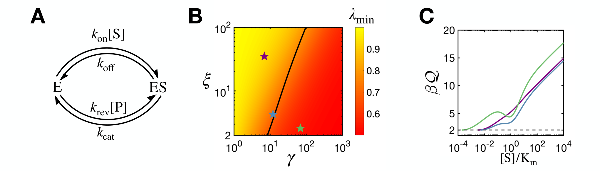
The suboptimal condition of reversible Michaelis-Menten reactions
We provide conditions at which has a local minimum with respect to substrate concentration () in reversible MM reactions shown in Fig. S2A. First, the affinity (),
| (S14) |
is a strictly increasing function of [S]. Next, the Fano factor () as a function of [S] is given by
| (S15) | ||||
| (S16) |
where and are dimensionless constants. has a local minimum only when , or equivalently, when . At the limit of a strongly driven catalytic step (), the expression for simplifies to
| (S17) |
which is minimized at with (Fig. S2B).
Since is monotonic with [S], a local minimum of can only occur near to that of . Using this, we numerically determined the range of and values at which has a local minimum away from the DB condition. For any , there exists a above which is non-monotonic (Fig. S2B). Thus, when and is sufficiently larger than , has a local minimum around .
Mathematical expressions of and for general copying processes
Here, we provide the details of obtaining and in the main text. A more mathematically rigorous treatment on the subject can be found in Ref. Pigolotti and Sartori 2016.
In the following, without loss of generality, we will define the error probability () and affinity () of copy processes by referring to the kinetic mechanism of mRNA translation. To begin, consider the ribosome at position of the mRNA sequence, decoding a specific codon type. For each amino-acid type , there exists a set , of associated aa-tRNAs, each of which represents a separate kinetic path of incorporating into the protein. If the codon at position is GGG, amino-acids Gly, Ala, Arg, Glu, Trp, and Val can be polymerized, with the following set of associated tRNAs: , , , , and (Fig. S7).
At steady state, we assume that, , the probability of incorporating amino-acid at position , where the codon is specified, is given by
| (S18) |
where is the set of all amino-acids, and is the polymerization current of aa-tRNA .
Next, we define the affinity associated with polymerization using the previously discussed example of Gly incorporation at codon GGG. The polymerization affinity of Gly along the cognate kinetic path associated with is
| (S19) |
where , and [C] represents the concentration of the ternary complex (Fig. 3B). The term is required to account for the fact that Gly can be depolymerized at position only fraction of the time. Similarly, the affinity of incorporating Gly along the near-cognate kinetic path associated with is
| (S20) |
where , and . Generally, we denote the polymerization affinity of amino-acid associated with aa-tRNA by .
Next, we let and be the current and affinity of the futile cycle within the incorporation path of aa-tRNA associated with amino-acid . Denoting the net polymerization flux by , we can write the affinity of mRNA translation at position as
| (S21) |
For the Bennett model, which involves two types of monomers, with one incorporation pathway each, without any futile cycles, we recover Eq. S10. To estimate in the extended model of translation (Fig. 4), we sum the Shannon-entropy of each position along the protein sequence.
Computation of and
We will work through the process of calculating and in the T7 DNA polymerase model, for which we apply Koza’s method of calculating currents and fluctuations in kinetic networks Koza 1999. To simplify the notation, we will relabel the states in Fig. 2A by indices 1 through 5; i.e., , , , , and . Additionally, we will relabel the rate constants so that represents the rate of the reaction from state to ; i.e., , , and so forth. Here, the depolymerization rate constants are set to and .
To begin, we will compute the current of correct nucleotide incorporation . For the -th chemical state (, where ) at time , let be the generalized state of the system after completing correct nucleotide incorporation cycles. Then, let be the probability of the system to be in state at time . The time evolution of is given by
| (S22) |
where the index runs through all states one reaction away from state . Here, the periodicity of the network model constrains the rate constants so that for and . Following Ref. Koza 1999, we define as
| (S23) |
where
for . By multiplying to both sides of Eq. S22 and using the equality , we get
| (S24) |
To derive the expression of as a function of the rate constants, we define the generating function
| (S25) |
where is the coordinate for the correct nucleotide incorporation cycle at state . Then, the time derivative of the generating function can be written as
| (S26) |
where the matrix is defined as
and also shown in the matrix form below
| (S27) |
For the computation of , is defined as
| (S28) |
Next, we define and denote the coordinate of the correct incorporation cycle by . Then, it can be shown that
| (S29) |
and
| (S30) |
where denotes the maximum eigenvalue of the matrix . Now, let denote the coefficients of the characteristic polynomial of (i.e., ). Then, we can write the following expressions for and ,
| (S31) | ||||
| (S32) |
where denotes the derivative with respect to evaluated at , and and are evaluated at . We can analogously compute the current of incorrect monomer incorporation, , by constructing the corresponding matrix , in which the non-diagonal entries of and are multiplied by and , respectively. Since and are functions of , and are functions of . Thus, we can solve for by the equality
| (S33) |
After we obtain the numerical expression of , we can construct the matrix to calculate the total flux and its fluctuation . With known values of and , the affinity of replication ( ) can be computed by Eq. S21. In sum, we have demonstrated how to calculate for the T7 DNA polymerase model.
We can calculate and of the simplified ribosome model in a similar way. To obtain as a function of , we construct the corresponding matrix , in which we multiply the non-diagonal entries corresponding to and by and , respectively. The expression for is obtained analogously, by constructing the corresponding matrix . After solving for the numerical value of the error probability, we can calculate the total polymerization rate and its fluctuation by constructing the corresponding matrix . When computing the affinity, we must also include the contribution from the futile cycle fluxes. To calculate the futile cycle current , we construct the corresponding matrix , in which we multiply the non-diagonal entries corresponding to , , and by , , and , respectively. Finally, the affinity of translation can be computed by Eq. S21.
Stochastic simulation of DNA replication
We simulated the replication of the first 300 base pairs of the T7 DNA polymerase gene sequence at the single molecule level, with Gillespie’s algorithm Gillespie 1977. The simulation starts with the polymerase in the apo state at the 5’ end of the gene sequence. The only reactions available at this state are the binding reactions of the 4 dNTPs, which are assumed to be at equal concentrations. After the binding of a dNTP, the simulation trajectories are generated based on the kinetic network shown in Fig. 2A. After each polymerization reaction, the polymerase translocates on the DNA and reads the next nucleotide. The simulation is terminated when the nucleotide of the gene sequence is polymerized.
The dynamics of DNA replication simulations are studied using the ensemble of trajectories generated. The total number of steps () in completing the replication of the DNA sequence varies from one realization to another. Selecting the completion time of replication () as the output observable for each realization, we define TUR of replication as
| (S34) |
where the dissipation has contributions from the free energy drive () and Shannon-entropy (). Denoting the forward and reverse rate constants of each kinetic step by and for , we can compute the average free energy drive by , where denotes the average over the ensemble of realizations. The entropic contribution is computed as , where is the probability of incorporating one of the 4 types of dNTPs, at the -th position.
The ribosome model
We provide more details on the model of translation by the ribosome in Fig. 3. Our model is a modified version of that from Rudorf et. al. Rudorf et al. 2014, in which we combine all linear chains of consecutive and irreversible reactions into single reactions. For instance, consider two consecutive and irreversible reactions and , with respective rate constants and , defined among three states , and . If there are no other reactions associated with the state , we remove the state , and define a new reaction with the rate constant .
To calculate the entropy productions, we defined reverse rate constants for all reactions, which were constrained by the affinity of the corresponding kinetic cycle. We assumed that affinities of the parallel kinetic cycles for the cognate and near-cognate aa-tRNAs were identical. The affinity of the futile cycle () comes from GTP hydrolysis, which dissipates Berg et al. 2002. Therefore, we applied the following constraints, where .
| (S35) | ||||
| (S36) |
The affinity involved with polymerization () can be estimated as the sum of the free energies of GTP hydrolysis, peptide bond formation, and the cleavage of the ester bond between the tRNA and the amino-acid. The hydrolysis of the GTP molecule incurs the dissipation of . Conversely, each peptide bond synthesized stores of free energy Martin 1998. The standard free energy of the ester bond between the amino-acid and the tRNA is Loftfield 1972; Berg et al. 2002. Since the ratio of charged to uncharged tRNAs is fold Evans et al. 2017, the net free energy of the ester bond between the amino-acid and tRNA is . Then, , which gives the following constraints
| (S37) | ||||
| (S38) |
The terms and implicitly take into account the concentration of tRNA and (EF-Tu)-GDP, which detach during the final polymerization step. In order to fully constrain all the rate constants, we set and . Modest changes to these affinity related constraints (Eqs S35-S38) do not affect the qualitative conclusions of our work.
Ternary complex concentration
The ternary complex concentration was modeled as a function of the concentration of its components, aa-tRNA, EF-Tu, GTP, and GDP. First, EF-Tu binds with GTP and GDP to form (EF-Tu)-GTP and (EF-Tu)-GDP, respectively. Then, aa-tRNA binds with (EF-Tu)-GTP and (EF-Tu)-GDP to form (aa-tRNA)-(EF-Tu)-GTP and (aa-tRNA)-(EF-Tu)-GDP, respectively Romero et al. 1985. Here, (aa-tRNA)-(EF-Tu)-GTP and (aa-tRNA)-(EF-Tu)-GDP represent the combined total of all the respective 42 individual ternary complexes. Assuming equilibrium, we can write the following equalities,
| (S39) | ||||
| (S40) | ||||
| (S41) | ||||
| (S42) |
where the respective dissociation constants are set to . Using Eqs. S39-S42, we can solve for the concentration of all chemical species given the total [EF-Tu], [aa-tRNA], [GTP], and [GDP]. Unless specified otherwise, all the ribosome model plots (Figs. 3 and 4) are made at the cellular condition, with . At the cellular condition, the concentration of the GTP bound ternary complex is .
Assuming that all species of aa-tRNA were bound to (EF-Tu)-GTP and (EF-Tu)-GDP with equal binding constants and , we computed the concentration of individual ternary complexes by referencing the measured concentration ratios among individual aa-tRNA species. For instance, the concentration of the cognate ternary complexes of codon UUU, which encodes for Phe, are
| (S43) | ||||
| (S44) |
where the subscript WT represents the cellular concentrations obtained from Ref. Dong et al. 1996.

The extended model of translation
Excluding the three stop codons, there are 61 types of codons encoding for 20 amino-acids. For E. coli, the 43 types of tRNAs were identified by Dong et. al Dong et al. 1996. Out of these, the pairs Gly1-Gly2 and Ile1-Ile2 were not differentiated in the concentration measurements. In our simulations, we assumed that Gly1 and Gly2 (resp. Ile1 and Ile2) were each present in the cellular milieu at half of the measured concentration of the Gly1-Gly2 pair (resp. Ile1-Ile2 pair). We removed the seleno-cysteine carrying tRNA from the analysis, since it is low in concentration, and it is incorporated into the polypeptide through a different kinetic scheme from the rest of the aa-tRNAs. Overall, we included total 42 types of aa-tRNAs in the extended translation model, with measurements from E. coli dividing every 86 minutes Dong et al. 1996. The cognate, near-cognate, and non-cognate groupings of aa-tRNAs for each codon is shown in Fig. S7.
mRNA translation by the ribosome at the single molecule level is simulated with Gillespie’s algorithm Gillespie 1977. The simulation starts with the ribosome in the apo state at the start codon. The only reactions available at this state are the bindings of the 42 aa-tRNAs, the concentrations of which were taken from Dong et. al. Dong et al. 1996. After the binding of an aa-tRNA, the simulation trajectories were generated on the kinetic network shown in Fig. 3B. After each polymerization reaction, the ribosome reads the next codon, translocating along the mRNA. The simulation is terminated when the ribosome completes the translation of the last codon.
The Hopfield model
We provide more details on the modified Hopfield model Hopfield 1974. The reaction cycle of the Hopfield model is composed of substrate binding ( and ), followed by the effectively irreversible steps of ATP hydrolysis ( and ) and polymerization ( and ) (Fig. S4). At states and , the substrate can also dissociate through the proofreading reaction (PR, and ), which is also effectively irreversible.
In the original formulation of the Hopfield model, the forward kinetic rate constants of correct and incorrect pathways were identical. In our modified version, the forward constants satisfy the following relations
| (S45) |
with . Next, to allow for error reduction by proofreading, we set the forward kinetic rates so that . Finally, we constrained the reverse reaction rates so that the affinities associated with the kinetic cycles are , and . The rate constants used to generate Fig. 5 and Fig. S9 are provided in Table S3.


