ManifoldNorm: Extending normalizations on Riemannian Manifolds

Rudrasis Chakraborty Affiliation: University of California Affiliation: Berkeley, CA, USA Email: rudrasischa@gmail.com

Abstract

Many measurements in computer vision and machine learning manifest as non-Euclidean data samples. Several researchers recently extended a number of deep neural network architectures for manifold valued data samples. Researchers have proposed models for manifold valued spatial data which are common in medical image processing including processing of diffusion tensor imaging (DTI) where images are fields of $3\times 3$ symmetric positive definite matrices or representation in terms of orientation distribution field (ODF) where the identification is in terms of field on hypersphere. There are other sequential models for manifold valued data that recently researchers have shown to be effective for group difference analysis in study for neuro-degenerative diseases. Although, several of these methods are effective to deal with manifold valued data, the bottleneck includes the instability in optimization for deeper networks. In order to deal with these instabilities, researchers have proposed residual connections for manifold valued data. One of the other remedies to deal with the instabilities including gradient explosion is to use normalization techniques including batch norm and group norm etc.. But, so far there is no normalization techniques applicable for manifold valued data. In this work, we propose a general normalization techniques for manifold valued data. We show that our proposed manifold normalization technique have special cases including popular batch norm and group norm techniques. On the experimental side, we focus on two types of manifold valued data including manifold of symmetric positive definite matrices and hypersphere. We show the performance gain in one synthetic experiment for moving MNIST dataset and one real brain image dataset where the representation is in terms of orientation distribution field (ODF).

1 Introduction

Geometric deep learning is a relatively nascent field which involves developing techniques to deal with manifold-valued samples, for example, a 2D matrix-valued image where at each pixel we have a matrix. Though traditional deep learning is an obvious choice for processing, in order to process structured matrices one needs to resort to sophisticated geometric tools. Recently, several researchers bronstein2017geometric; chakraborty2018statistical; cohen2019general; cohen2018spherical; cohen2019gauge; esteves2018learning; chakraborty2018cnn; kondor2018clebsch; sommer2019horizontal; chakraborty2018manifoldnet; kondor2018generalization proposed deep learning tools tailored for non-Euclidean data. There are two types of data domains applicable for manifold valued deep learning:

(1) each sample is a function on a manifold, i.e.,

X_{i}:\mathcal{M}\rightarrow\mathbf{R}

(2) each sample is manifold valued grid, i.e.,

X_{i}:\mathbf{Z}^{n}\rightarrow\mathcal{M}

. A special case for the second type of data domain is grayscale images where $n=2$ and $\mathcal{M}=\mathbf{R}$ .

Some of the recent works where the data domain is function on manifold include Spherical CNN cohen2018spherical; esteves2018learning; kondor2018clebsch, Homogeneous CNN chakraborty2018cnn; kondor2018generalization; cohen2019general. Cohen et al. cohen2018spherical extended the convolution operator on hypersphere and showed that the proposed convolution operator is equivariant to the group of rotations. In Esteves et al. esteves2018learning, the authors proposed a different way to do spherical convolution by using the definition proposed by Driscoll and Healy driscoll1994computing. Their proposed convolution is equivariant to planar rotations. In chakraborty2018cnn; cohen2019general; kondor2018generalization, the authors proposed a more general definition of convolution on a Riemannian homogeneous space and proved that their definition is equivariant to the group that naturally acts on the homogeneous space. Moreover, in cohen2019gauge, the authors went one step further and proposed a Gauge equivariant convolution operator.

Several researchers focused on the second type of data domain where each sample is a manifold valued grid. In chakraborty2018manifoldnet, the authors proposed a convolution neural network on a general Riemannian manifold. They proposed a definition of convolution equivariant to the isometry group acts on the underlying manifold. The authors proposed convolution, non-linearity and invariant fully connected layers. In this wok, we propose normalization layer appropriate for the formalism of CNN for a Riemannian manifold proposed in chakraborty2018manifoldnet. In bouza2020mvc, the authors proposed a CNN for manifold valued data based on defining convolution on tangent spaces. Several other researchers including chakraborty2018statistical proposed a statistical recurrent model for manifold valued sequential datasets.

One of the obstacles in defining deep neural network with a large number of layers is the explosion of gradient. Several “remedies” have been proposed including residual connection he2016deep, batch normalization ioffe2015batch. Recently, authors in zhen2019dilated proposed residual connections for convolutions on manifold valued data and have achieved more stable optimization technique. This motivates us to define normalization techniques on a general Riemannian manifold. In brooks2019riemannian, the authors proposed batch normalization for manifold of symmetric positive definite matrices. In this work, we generalize the work in two ways

(a) we extend normalization technique for a Riemannian manifold (b) moreover, inspired by the recent work of group normalization wu2018group, we define group normalization for a general Riemannian manifold.

In this work, our contribution is as follows:

(a) we propose a Riemannian group normalization technique appropriate for Riemannian homoegenous spaces (b) we prove for matrix Lie groups our proposed group normalization satisfies the desired first and second order moments (c) proof of concept type experiments show the performance gain of our proposed method over several state-of-the-art manifold valued baselines.

2 Preliminaries

This section is intended for a very brief summarization of some differential geometric terminologies we are going to use in the rest of the paper. For a more concrete treatment, the readers are encouraged to look at boothby1986introduction.

Definition 1 (Riemannian manifold and metric).

Let $(\mathcal{M},g^{\mathcal{M}})$ be a orientable complete Riemannian manifold with a Riemannian metric $g$ , i.e., $\forall x\in\mathcal{M}:g_{x}:T_{x}{\mathcal{M}}\times T_{x}{\mathcal{M}}\rightarrow\mathbf{R}$ is a bi-linear symmetric positive definite map, where $T_{x}\mathcal{M}$ is the tangent space of $\mathcal{M}$ at $x\in\mathcal{M}$ . Let $d:\mathcal{M}\times\mathcal{M}\rightarrow[0,\infty)$ be the distance induced from the Riemannian metric $g$ .

Definition 2.

Let $p\in\mathcal{M}$ , $r>0$ . Define $\mathcal{B}_{r}(p)=\left\{q\in\mathcal{M}|d(p,q)<r\right\}$ to be a open ball at $p$ of radius $r$ .

Definition 3 (Local injectivity radius groisser2004newton).

The local injectivity radius is defined as $r_{\text{inj}}(p)=\sup\left\{r|\text{Exp}_{p}:(\mathcal{B}_{r}(\mathbf{0})\subset T_{p}\mathcal{M})\rightarrow\mathcal{M}\text{ is defined}\right.$ and is a diffeomorphism $\left.\text{onto its image}\right\}$ at $p\in\mathcal{M}$ . The injectivity radius manton2004globally of $\mathcal{M}$ is defined as $r_{\text{inj}}(\mathcal{M})=\inf_{p\in\mathcal{M}}\left\{r_{\text{inj}}(p)\right\}$ .

Within $\mathcal{B}_{r}(p)$ , where $r\leq r_{\text{inj}}(\mathcal{M})$ , the mapping $\text{Exp}^{-1}_{p}:\mathcal{B}_{r}(p)\rightarrow\mathcal{U}\subset T_{p}\mathcal{M}\subset\mathbf{R}^{m}$ , is called the inverse Exponential/Log map, $m$ is the dimension of $\mathcal{M}$ .

Definition 4.

Given $p,q\in\mathcal{U}\subset\mathcal{B}_{r}(p)$ , where $r\leq r_{\text{inj}}(\mathcal{M})$ , the (shortest) geodesic is the smooth curve $\Gamma:[0,1]\rightarrow\mathcal{M}$ with $\Gamma(0)=p$ , $\Gamma(1)=q$ and $d(p,q)=\int_{[0,1]}\sqrt{g_{\Gamma(t)}\left(\frac{d\Gamma}{dt},\frac{d\Gamma}{dt}\right)}dt$ .

there exists a unique length minimizing geodesic segment between $p$ and $q$ and the geodesic segment lies entirely in $\mathcal{U}$ .

Definition 5.

chavel1984eigenvalues $\mathcal{U}\subset\mathcal{M}$ is strongly convex if for all $p,q\in\mathcal{U}$ , there exists a unique length minimizing geodesic segment between $p$ and $q$ and the geodesic segment lies entirely in $\mathcal{U}$ .

Definition 6.

groisser2004newton Let $p\in\mathcal{M}$ . The local convexity radius at $p$ , $r_{\text{cvx}}(p)$ , is defined as $r_{\text{cvx}}(p)=\sup\left\{r\leq r_{\text{inj}}(p)|\mathcal{B}_{r}(p)\text{ is strongly convex}\right\}$ . The convexity radius of $\mathcal{M}$ is defined as $r_{\text{cvx}}(\mathcal{M})=\inf_{p\in\mathcal{M}}\left\{r_{\text{cvx}}(p)\right\}$ .

In rest of the paper, we assume data points are within the geodesic ball of radius less than $\min\{r_{\text{inj}}(\mathcal{M}),r_{\text{cvx}}(\mathcal{M})\}$ .

Definition 7 (Group of isometries of $\mathcal{M}$ ( $I\left(\mathcal{M}\right)$ )).

A diffeomorphism $\phi:\mathcal{M}\rightarrow\mathcal{M}$ is an isometry if it preserves distance, i.e., $d\left(\phi\left(x\right),\phi\left(y\right)\right)=d\left(x,y\right)$ . The set $I(\mathcal{M})$ of all isometries of $\mathcal{M}$ forms a group with respect to function composition.

Rather than write an isometry as a function $\phi$ , we will write it as a group action. Henceforth, let $G$ denote the group $I(\mathcal{M})$ , and for $g\in G$ , and $x\in\mathcal{M}$ , let $g\cdot x$ denote the result of applying the isometry $g$ to point $x$ .

Definition 8 (Riemannian homogeneous spaces helgason2001differential).

Given $\mathcal{M}$ and $G$ as defined above, let $G$ acts transitively on $\mathcal{M}$ , i.e., given $p,q\in\mathcal{M}$ , $\exists g\in G$ , such that $q=g\cdot p$ . Let $H=\textsf{Stab}(I)$ , where $I$ is the “origin” of $\mathcal{M}$ where $\textsf{Stab}(I)=\left\{g\in G|g\cdot I=I\right\}$ is the stabilizer of $I$ . Then $\mathcal{M}$ is a Riemannian homogeneous space and can be identified as the quotient space $G/H$ .

Some of the examples of Riemannian homogeneous spaces include Euclidean space, hypersphere, hyperbolic space, Lie groups (will be defined next).

Definition 9 (Lie group hall2015lie).

$\mathcal{M}$ is called a Lie group if

(a)

\mathcal{M}

is a group with the group operation

\circ

(b) the group operations

(g,h)\mapsto g\circ h

and

g\mapsto g^{-1}

are smooth.

Definition 10 (Lie algebra hall2015lie).

The tangent space of $\mathcal{M}$ at identity, $I$ , i.e., $T_{I}\mathcal{M}$ is a vector space and is termed as Lie algebra, $\mathfrak{M}$ . Lie algebra is a vector space.

Observe the basic properties of a matrix Lie group, $\mathcal{M}$ :

(a) the distance on

\mathcal{M}

can be defined as

d(X,Y)=\|\textsf{logm}\left(X^{-1}Y\right)\|

, here logm is the matrix logarithm and

\|.\|

is the Frobenius norm (b)

\textsf{logm}:\mathcal{M}\rightarrow\mathfrak{m}

is the mapping from Lie group to Lie algebra and expm is the inverse of this mapping (c) Given

X,Y\in\mathcal{M}

, the shortest geodesic from

X

Y

is given by

\Gamma_{X}^{Y}(t)=X\textsf{expm}\left(t\textsf{logm}\left(X^{-1}Y\right)\right)

In the rest of the paper, we assume $\mathcal{M}$ to be a Riemannian homogeneous space. Moreover, we will assume $\mathcal{M}$ is associated with the Levi-Civita connection: $\nabla:V_{\mathcal{M}}\times V_{\mathcal{M}}\rightarrow V_{\mathcal{M}}$ where $V_{\mathcal{M}}$ is the space of vector fields on $\mathcal{M}$ boothby1986introduction.

Now, we give some definitions including Parallel transport, Fréchet mean which are needed in order to define Riemannian normalization.

Definition 11 (Parallel transport on $\mathcal{M}$ ( $\Gamma_{p\rightarrow q}\left(\mathbf{v}\right)$ )).

Let $p,q\in\mathcal{M}$ and $\mathbf{v}\in T_{p}\mathcal{M}$ . Let $\gamma:[0,1]\rightarrow\mathcal{M}$ be the (shortest) geodesic with $\gamma(0)=p$ and $\gamma(1)=q$ . A vector field $V$ is said to be parallel transport of $\mathbf{v}$ along $\gamma$ provided that $\left\{V(t),t\in[0,1]\right\}$ is a vector field for which $V(0)=\mathbf{v}$ . We assign $V(1)\in T_{q}\mathcal{M}$ to be $\Gamma_{p\rightarrow q}\left(\mathbf{v}\right)$ .

Note that the term parallel is because of $\nabla_{\gamma^{\prime}(t)}V(t)|_{t_{0}}=0$ , for all $t_{0}\in[0,1]$ .

Definition 12 (weighted Fréchet mean).

Given $\left\{X_{i}\right\}_{i=1}^{N}\subset\mathcal{M}$ , and a set of weights $\left\{w_{i}\right\}_{i=1}^{N}\subset(0,1]$ with $\sum_{i=1}^{N}w_{i}=1$ (i.e., $\left\{w_{i}\right\}$ satisfy convexity constraint), we can define “the” weighted Fréchet mean (wFM) frechet1948elements as the minimizer of the weighted variance, i.e.,

\textsf{wFM}\left(\left\{X_{i}\right\},\left\{w_{i}\right\}\right)=\argmin_{M\in\mathcal{M}}\sum_{i=1}^{N}w_{i}d^{2}(X_{i},M).

We use the following proposition afsari2011riemannian to argue that if the samples are within the geodesic ball of aforementioned radius, then the wFM exists and is unique. Note that if $w_{i}=\nicefrac{{1}}{{N}}$ , for all $i$ , then we get “the” Fréchet mean (FM) defined as

\displaystyle\textsf{FM}\left(\left\{X_{i}\right\}\right)=\argmin_{M\in\mathcal{M}}\sum_{i=1}^{N}d^{2}(X_{i},M).

(1)

Given $\left\{X_{i}\right\}_{i=1}^{N}\subset\mathcal{M}$ we will use a provably convergent recursive estimator of wFM as proposed in Chakraborty et al. chakraborty2018manifoldnet. The recursive wFM estimator, $M_{N}$ , is defined as

\displaystyle M_{1}=X_{1}\qquad\qquad M_{n+1}=\Gamma_{M_{n}}^{X_{n+1}}\left(\frac{w_{n+1}}{\sum_{j=1}^{n+1}w_{j}}\right)

(2)

Recently in chakraborty2018manifoldnet, the authors proposed a manifold valued deep neural network where they defined convolution operator using wFM. In the next section, we first formally define Riemannian normalization before recalling the definition of convolution.

3 Riemannian normalization

In this section, we formulate a general normalization scheme on a Riemannian manifold. We propose algorithms for normalization on a general homogeneous space and a Lie group in the subsequent subsections. Before that we formulate the problem of Riemannian normalization in a general form and show that the popular batch normalization, group normalization, layer norm are special cases of our formulation when the manifold is an Euclidean space.

Definition 13 (Riemannian normalization).

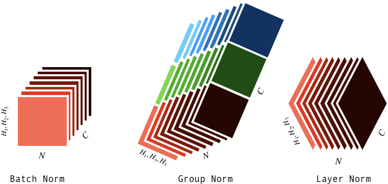
Given $\left\{X_{i_{1},i_{2},i_{3},i_{n},i_{c}}\right\}\subset\mathcal{M}$ with indices $i1,i2,i3$ run over the spatial 3D dimension (correspond to three dimension of a 3D volume), $i_{n}$ and $i_{c}$ are the indices over the number of samples and number of channels respectively, the Riemannian normalization normalize the first order and second order moments over specific index (or a set of indices). Let $\mathcal{S}$ be the set over which we desire to perform the normalization. Depending on the construction of the set $\mathcal{S}$ we get different types of normalization. As for an example, if $\mathcal{S}=\left\{X_{i_{1},i_{2},i_{3},i_{n},i_{c}}|i_{c}=c\right\}$ then it is batch normalization, here $c$ is a channel index $c$ . In other words, the batch normalization is over $\left\{(i_{1},i_{2},i_{3},i_{n})\right\}$ indices.

Given a set $\mathcal{S}$ , the Riemannian normalization tries to fit a distribution with desired first and second order moments. Before formally defining distribution on a Riemannian homogeneous space, we first give examples of different kinds of Riemannian normalization, i.e., different choices of $\mathcal{S}$ .

(a)

Riemannian batch normalization: If $\mathcal{S}=\left\{X_{i_{1},i_{2},i_{3},i_{n},i_{c}}|i_{c}=c\right\}$ for a channel $c$ , then the normalization is termed as Riemannian batch normalization. Hence, the batch normalization is over $\left\{(i_{1},i_{2},i_{3},i_{n})\right\}$ indices.
(b)

Riemannian layer normalization: If $\mathcal{S}=\left\{X_{i_{1},i_{2},i_{3},i_{n},i_{c}}|i_{n}=n\right\}$ for a sample $n$ , then the normalization is termed as Riemannian layer normalization. Hence, the layer normalization is over $\left\{(i_{1},i_{2},i_{3},i_{c})\right\}$ indices.
(c)

Riemannian instance normalization: If $\mathcal{S}=\left\{X_{i_{1},i_{2},i_{3},i_{n},i_{c}}|i_{c}=c,i_{n}=n\right\}$ for a channel $c$ and sample $n$ , then the normalization is termed as Riemannian instance normalization. Hence, the instance normalization is over $\left\{(i_{1},i_{2},i_{3})\right\}$ indices.
(d)

Riemannian group ormalization: If $\mathcal{S}=\left\{X_{i_{1},i_{2},i_{3},i_{n},i_{c}}|i_{n}=n,i_{c}\in C_{g}\right\}$ for a sample $n$ and a channel group $C_{g}=\{c_{1},\cdots,c_{n}\}$ , then the normalization is termed as Riemannian group normalization. Hence, the group normalization is over $\left\{(i_{1},i_{2},i_{3},i_{c})\right\}$ indices but $i_{c}$ is over a group of channels $C_{g}$ .

A visual description of different kind of Riemannian normalization is shown in Fig. (1).

Refer to caption — Figure 1: Pictorial description of various kind of Riemannian normalization.

3.1 Riemannian homogeneous spaces

In this subsection, we assume $\mathcal{M}$ to be a Riemannian homogeneous space of dimension $m$ . We assume the distance $d$ used is induced by the $G$ -invariant Riemannian metric where $G$ is the group transitively acts on $\mathcal{M}$ . Hence, the isometry group under this distance $d$ is the group $G$ . We use $\cdot$ to denote the group action as given by $(g,M)\mapsto g\cdot M$ , where, $g\cdot M\in\mathcal{M}$ .

Let $M\in\mathcal{M}$ , there exists an isomorphism $\iota:T_{M}\mathcal{M}\rightarrow\mathbf{R}^{m}$ from the tangent space at $M$ to the Euclidean space $\mathbf{R}^{m}$ . Now, we are ready to give the definition of Gaussian distribution.

Definition 14 (Gaussian distribution pennec2004probabilities).

Given a Riemannian homogeneous space $\mathcal{M}$ (of dimension $m$ ) with the distance $d$ and group $G$ acts of $\mathcal{M}$ , we can define Gaussian distribution with location parameter $M$ and concentration matrix $\Delta$ as:

\displaystyle f(X|M;\Delta)

\displaystyle=k\exp\left(-\frac{\mathbf{v}^{t}\Delta\mathbf{v}}{2}\right)

(3)

where the normalization constant $k$ and the covariance matrix $\Sigma$ are given as follows.

k^{-1}=\int_{\mathcal{M}}\exp\left(-\frac{\mathbf{v}^{t}\Delta\mathbf{v}}{2}\right)\omega(X)

\Sigma=k\int_{\mathcal{M}}\mathbf{v}\mathbf{v}^{t}\exp\left(-\frac{\mathbf{v}^{t}\Delta\mathbf{v}}{2}\right)\omega(X)

here, $\omega:\mathcal{M}\rightarrow[0,\infty)$ is the Riemannian volume density and $\mathbf{v}=\textsf{Exp}^{-1}_{M}(X)$ . This definition amounts to defining truncated Gaussian distribution of the exponential chart map.

Given a set $\mathcal{S}$ of samples on which we need to apply normalization, in Alg. (1) which present the training step of Riemannian normalization.

Input: A batch of samples

\mathcal{S}=\left\{X_{i}\right\}_{i=1}^{N}

; bias

g\in G

; running mean

M

; positive diagonal scaling matrix

S\in\mathbf{R}^{m\times m}

Output: updated running mean

M

Compute batch mean,

M_{b}

\left\{X_{i}\right\}_{i=1}^{N}

using Riemannian metric (incremental FM in Eq. (2)); 1

Update running mean

M

M_{b}

(incremental FM in Eq. (2)); 2

X_{i}\leftarrow\textsf{Exp}\left(\Gamma_{M_{b}\rightarrow I}\left(\mathbf{v}_{i}\right)\right)

, where

\mathbf{v}_{i}=\textsf{Exp}^{-1}_{M_{b}}\left(X_{i}\right)

; 3

X_{i}\leftarrow\textsf{Exp}\left(\iota^{-1}\left(S\iota\left(\mathbf{v}_{i}\right)\right)\right)

, where

\mathbf{v}_{i}=\textsf{Exp}^{-1}_{I}\left(X_{i}\right)

; 4

X_{i}\leftarrow g\cdot X_{i}

. 5

Algorithm 1 Training step of normalization on a Riemannian homogeneous space

In Alg. (2), we present the testing algorithm. Notice that in training algorithm, we update the running mean of the distribution, while for testing algorithm we use the final learned running mean $M$ .

Input: A batch of samples

\mathcal{S}=\left\{X_{i}\right\}_{i=1}^{N}

; bias

g\in G

; learned running mean

M

; diagonal scaling matrix

S

X_{i}\leftarrow\textsf{Exp}\left(\Gamma_{M\rightarrow I}\left(\mathbf{v}_{i}\right)\right)

, where

\mathbf{v}_{i}=\textsf{Exp}^{-1}_{M}\left(X_{i}\right)

; 1

X_{i}\leftarrow\textsf{Exp}\left(\iota^{-1}\left(S\iota\left(\mathbf{v}_{i}\right)\right)\right)

, where e

\mathbf{v}_{i}=\textsf{Exp}^{-1}_{I}\left(X_{i}\right)

; 2

X_{i}\leftarrow g\cdot X_{i}

. 3

Algorithm 2 Testing step of normalization on a Riemannian homogeneous space

Note that, the parallel translate operation does not guarantee the FM of the samples in $\mathcal{S}$ , as given the mean $M$ and the desired mean $I$ , although there exists a group element $g_{M}\in G$ such that $g_{M}\cdot I=M$ (as a property of the Riemannian homogeneous space), $g_{M}$ does not have a closed form in general. Hence, we will focus on a subclass of Riemannian homogeneous spaces, namely Lie groups, where because of the group inverses we can get a closed form of $g_{M}$ .

Note that, the above algorithms can be applicable to a general Riemannian manifold $\mathcal{M}$ with closed form for geodesic, parallel transport and we will use $G=I(\mathcal{M})$ , the isometry group. Before giving the formulation for Lie groups, we present two examples of homogeneous spaces with the appropriate operations needed for Riemannian normalization.

3.1.1 Riemannian homogeneous spaces: some examples

SPD

: Let $\mathcal{M}$ be the manifold of $n\times n$ symmetric positive definite matrices with affine-invariant metric. Below, we give closed form of the operations needed in the normalization algorithm.

(a)

Distance: $d(X,Y)=\|\textsf{logm}\left(X^{-1}Y\right)\|$ .
(b)

$G$ : The group that acts on $\mathcal{M}$ (isometry group) is $G=\textsf{GL}(n)$ , $n\times n$ invertible matrices.
(c)

Group action: $g\cdot X\mapsto gXg^{T}$ .
(d)

Log map: $\textsf{Exp}^{-1}_{X}(Y)=X^{1/2}\textsf{logm}\left(X^{-1/2}YX^{-1/2}\right)X^{1/2}$ , where, $\textsf{logm}(Z)=U\log(D)U^{T}$ , where $Z=UDU^{T}$ .
(e)

Exp map: $\textsf{Exp}_{X}(V)=X^{1/2}\textsf{expm}\left(X^{-1/2}VX^{-1/2}\right)X^{1/2}$ , where, $\textsf{expm}(Z)=U\exp(D)U^{T}$ , where $Z=UDU^{T}$ .
(f)

Parallel transport: $\Gamma_{X\rightarrow Y}(V)=Y^{1/2}\left(X^{-1/2}VX^{-1/2}\right)Y^{1/2}$ .

$\mathbf{S}^{n}$

: Let $\mathcal{M}$ be $n$ -dimensional unit hypersphere with arc-length metric. Below, we give closed form of the operations needed in the normalization algorithm.

(a)

Distance: $d(\mathbf{x},\mathbf{y})=\arccos\left(\mathbf{x}^{t}\mathbf{y}\right)$ .
(b)

$G$ : The group that acts on $\mathcal{M}$ (isometry group) is $G=\textsf{SO}(n)$ , $n\times n$ special orthogonal matrices.
(c)

Group action: $g\cdot\mathbf{x}\mapsto g\mathbf{x}$ .
(d)

Log map: $\textsf{Exp}^{-1}_{\mathbf{x}}(\mathbf{y})=\frac{\sin(\theta)}{\theta\left(\mathbf{y}-\mathbf{x}\cos(\theta)\right)}$ , where $\theta=d(\mathbf{x},\mathbf{y})$ .
(e)

Exp map: $\textsf{Exp}_{\mathbf{x}}(\mathbf{v})=\cos(\|\mathbf{v}\|)\mathbf{x}+\sin(\|\mathbf{v}\|)\frac{\mathbf{v}}{\|\mathbf{v}\|}$ .
(f)

Parallel transport: $\Gamma_{\mathbf{x}\rightarrow\mathbf{y}}(\mathbf{v})=\left(\mathbf{v}-\mathbf{w}\frac{\mathbf{w}^{t}\mathbf{v}}{\|\mathbf{w}\|^{2}}\right)+\frac{\mathbf{w}^{t}\mathbf{v}}{\|\mathbf{w}\|^{2}}\left(\mathbf{x}\left(-\sin(\|\mathbf{w}\|)\|\mathbf{w}\|\right)+\mathbf{w}\cos(\|\mathbf{w}\|)\right)$ , where $\mathbf{w}=\textsf{Exp}^{-1}_{\mathbf{x}}\left(\mathbf{y}\right)$ .

3.2 Matrix Lie groups

In this subsection, we assume $\mathcal{M}$ to be matrix Lie group. As mentioned before, given $X,Y\in\mathcal{M}$ , we define the distance as $d(X,Y)=\|\textsf{logm}\left(X^{-1}Y\right)\|$ . Notice that, this metric invariant to the left group operation. Formally, given $Z\in\mathcal{M},d(ZX,ZY)=d(X,Y)$ . Hence, the isometry group, $G$ is given by $G=\mathcal{M}$ with respect to the left group operation.

Before defining normalization for matrix Lie groups, we first define Gaussian distribution for matrix Lie groups. Note that although the earlier definition of Gaussian distribution on a Riemannian homogeneous space can be applied here, here we gave a different definition of Gaussian distribution which can be used to define computationally more efficient Riemannian normalization for special cases of matrix Lie groups.

Definition 15 (Gaussian distribution chakraborty2019statistics).

Given a Riemannian homogeneous space $\mathcal{M}$ with the distance $d$ , induced from a Riemannian metric (and group $G$ acts of $\mathcal{M}$ ), we can define Gaussian distribution with location parameter $M\in\mathcal{M}$ and variance $\sigma^{2}>0$ , denoted by $\mathcal{N}\left(M,\sigma^{2}\right)$ as:

\displaystyle f(X|M,\sigma^{2})

\displaystyle=k(\sigma)\exp\left(-\frac{d(X,M)^{2}}{2\sigma^{2}}\right)

(4)

where, $k$ is the normalizing constant.

Before presenting the algorithm of Remannian normalization on matrix Lie groups, we first start with stating some propositions.

Proposition 1.

Given $\left\{X_{i}\right\}\subset\mathcal{M}$ i.i.d. samples drawn from $\mathcal{N}\left(M,\sigma^{2}\right)$ , the maximum likelihood estimator (MLE) of $M$ is the sample Fréchet mean (FM) of $\left\{X_{i}\right\}$ .

Proof.

From Eq. (4), we can get the log-likelihood, $\ell\left(M;\left\{X_{i}\right\},\sigma^{2}\right)$ as

\displaystyle\ell\left(M;\left\{X_{i}\right\},\sigma^{2}\right)=\log(k(\sigma))-\sum_{i=1}^{N}\frac{d(X_{i},M)^{2}}{2\sigma^{2}}

Now, maximizing $\ell\left(M;\left\{X_{i}\right\},\sigma^{2}\right)$ is equivalent to minimizing $\sum_{i=1}^{N}d(X_{i},M)^{2}$ . Hence, using Eq. (1), we can conclude that the MLE of $M$ is the FM of $\left\{X_{i}\right\}$ . ∎

Now, using the MLE and FM equivalence as showed in Prop. (1), we can state the following proposition.

Proposition 2.

Given $X\sim\mathcal{N}\left(M,\sigma^{2}\right)$ with parameters $M\in\mathcal{M}$ and $\sigma^{2}>0$ , $ZX\sim\mathcal{N}\left(ZM,\sigma^{2}\right)$ , for all $Z\in\mathcal{M}$ .

Proof.

In order to prove the proposition it is sufficient to show that $f(X|M,\sigma^{2})=cf(ZX|ZM,\sigma^{2})$ using Eq. (4) in Def. (15) for some constant $c>0$ . Observe that,

	$\displaystyle f(ZX\|ZM,\sigma^{2})$	$\displaystyle=k(\sigma)\exp\left(-\frac{d(ZX,ZM)^{2}}{2\sigma^{2}}\right)$
		$\displaystyle=k(\sigma)\exp\left(-\frac{\\|\textsf{logm}\left(X^{-1}Z^{-1}ZM\right)\\|^{2}}{2\sigma^{2}}\right)$
		$\displaystyle=f(X\|M,\sigma^{2})$

∎

Proposition 3.

Given $X\sim\mathcal{N}\left(I,\sigma^{2}\right)$ with parameters $I\in\mathcal{M}$ ( $I$ to be the identity element) and $\sigma^{2}>0$ , then $Y:=\textsf{expm}\left(s\textsf{logm}\left(X\right)\right)\sim\mathcal{N}\left(I,s^{2}\sigma^{2}\right)$ , for all $Z\in\mathcal{M}$ for all $s>0$ .

Proof.

Similar to before, it is sufficient to show that $f(X|I,\sigma^{2})=cf(Y|I,s^{2}\sigma^{2})$ where, $Y=\textsf{expm}\left(s\textsf{logm}\left(X\right)\right)$ , for some constant $c$ . Observe that,

	$\displaystyle f(Y\|I,s^{2}\sigma^{2})$	$\displaystyle=k(s\sigma)\exp\left(-\frac{d(Y,I)^{2}}{2s^{2}\sigma^{2}}\right)$
		$\displaystyle=k(s\sigma)\exp\left(-\frac{\\|\textsf{logm}\left(Y\right)\\|^{2}}{2s^{2}\sigma^{2}}\right)$
		$\displaystyle=k(s\sigma)\exp\left(-\frac{\\|\textsf{logm}\left(X\right)\\|^{2}}{2\sigma^{2}}\right)$
		$\displaystyle=cf(X\|I,\sigma^{2})$

for some $c>0$ . ∎

As a corollary of Prop. (3), we can state the following.

Proposition 4.

Given $\left\{X_{i}\right\}_{i=1}^{N}\subset\mathcal{M}$ and $\left\{w_{i}\right\}$ satisfying convexity constraint, let $I=\textsf{wFM}\left(\left\{X_{i}\right\},\left\{w_{i}\right\}\right)$ be the wFM. Then, for all $s>0$ , $I=\textsf{wFM}\left(\left\{Y_{i}\right\},\left\{w_{i}\right\}\right)$ be the wFM of $\left\{Y_{i}\right\}$ , where, $Y_{i}\textsf{expm}\left(s\textsf{logm}\left(X_{i}\right)\right)$ .

Proof.

\displaystyle\sum_{i=1}^{N}w_{i}d^{2}(Y_{i},I)

\displaystyle=s^{2}\sum_{i=1}^{N}w_{i}d^{2}(X_{i},I)

Hence, $I$ to be wFM of $\left\{X_{i}\right\}$ if and only if $I$ to be wFM of $\left\{Y_{i}\right\}$ . ∎

Using Props. (3) and (4) we can propose our formulation of normalization in Alg. (3). Before giving the testing algorithm, we like to discuss some key points of Alg. (3) as listed next.

(a) In line 3, we adjust the batch mean to be

I

(the identity element of

\mathcal{M}

) (b) In line 4, the batch mean remains unchanged (courtesy of Prop. 4) but the scaling parameter of the distribution is scaled as stated in Prop. 3 (c) In line 5, we change the batch mean from

I

g

Input: A batch of samples

\mathcal{S}=\left\{X_{i}\right\}_{i=1}^{N}

; bias

g\in\mathcal{M}

(here

G=\mathcal{M}

as Lie group); running mean

M

; scale factor

s>0

Output: updated running mean

M

Compute batch mean,

M_{b}

\left\{X_{i}\right\}_{i=1}^{N}

using Riemannian metric (incremental FM in Eq. (2)); 1

Update running mean

M

M_{b}

(incremental FM in Eq. (2)); 2

X_{i}\leftarrow M_{b}^{-1}X_{i}

; 3

X_{i}\leftarrow\textsf{expm}\left(s\textsf{logm}\left(X_{i}\right)\right)

; 4

X_{i}\leftarrow gX_{i}

. 5

Algorithm 3 Training step of normalization on a Lie group

The testing algorithm is similar to before and is presented next in Alg. (4). The testing algorithm inputs the updated running mean $M$ and bias $g$ and scale $s$ from training algorithm in Alg. (3) and changes the distribution of the test samples accordingly.

Input: A batch of samples

\mathcal{S}=\left\{X_{i}\right\}_{i=1}^{N}

; bias

g\in\mathcal{M}

; learned running mean

M

; scale factor

s>0

X_{i}\leftarrow M^{-1}X_{i}

; 1

X_{i}\leftarrow\textsf{expm}\left(s\textsf{logm}\left(X_{i}\right)\right)

; 2

X_{i}\leftarrow gX_{i}

. 3

Algorithm 4 Testing step of normalization on a Lie group

Now, we present some examples of matrix Lie groups.

3.2.1 Lie groups: some examples

SPD

: Let $\mathcal{M}$ be the manifold of $n\times n$ symmetric positive definite matrices with log-Euclidean metric. As shown in arsigny2006log, SPD with log-Euclidean metric is a matrix Lie group. Below, we give closed form of the operations needed in the normalization algorithm.

(a)

Distance: $d(X,Y)=\|\textsf{logm}(X)-\textsf{logm}(Y)\|$ .
(b)

$G$ : The group that acts on $\mathcal{M}$ (isometry group) is $G=\textsf{SO}(n)$ , $n\times n$ special orthogonal matrices.
(c)

Group action: $g\cdot X\mapsto gXg^{T}$ .
(d)

Log map: $\textsf{Exp}^{-1}_{X}(Y)=\textsf{logm}(Y)-\textsf{logm}(X)$ .
(e)

Exp map: $\textsf{Exp}_{X}(V)=\textsf{expm}\left(V+\textsf{logm}(X)\right)$ .

SO

: Let $\mathcal{M}$ be the manifold of $n\times n$ special orthogonal matrices. Below, we give closed form of the operations needed in the normalization algorithm.

(a)

Distance: $d(X,Y)=\|\textsf{logm}(X^{T}Y)\|$ .
(b)

$G$ : The group that acts on $\mathcal{M}$ (isometry group) is $G=\textsf{SO}(n)$ .
(c)

Group action: $g\cdot X\mapsto gX$ .
(d)

Log map: $\textsf{Exp}^{-1}_{X}(Y)=X\textsf{logm}(X^{T}Y)$ .
(e)

Exp map: $\textsf{Exp}_{X}(V)=X\textsf{expm}\left(X^{T}V\right)$ .
(f)

Parallel transport: $\Gamma_{X\rightarrow Y}(V)=YX^{T}V$ .

3.3 Architecture for network with manifold normalization

In this section, we present the basic building blocks for manifold valued deep learning:

(a) the ManifoldConv layer as proposed in chakraborty2018manifoldnet using wFM operator proposed in Eq. (2) (b) tangent ReLU (tReLU) as non-itineraries (c) manifold normalization block (d) manifold valued fully connected (ManifoldFC) layer

. For completeness, we present the definition of manifoldconv, tReLU and manifoldfc blocks here.

ManifoldConv: Given $\{X_{i}\|_{i=1}^{N}$ and weights (to be learned) $\{w_{i}\}_{i=1}^{N}$ satisfying convexity constraint, the output of ManifoldConv is $\textsf{wFM}\left(\{X_{i}\},\{w_{i}\}\right)$ as defined in Eq. (2).

tReLU: This layer takes $X\in\mathcal{M}$ as input and returns $\textsf{Exp}_{I}\left(\text{ReLU}\left(\textsf{Exp}^{-1}_{I}\left(X\right)\right)\right)$ .

ManifoldFC: Given $\{X_{i}\|_{i=1}^{N}$ as input, ManifoldFC returns $\{d(X_{i},M)\}_{i=1}^{N}\subset\mathbf{R}$ , where $M=\textsf{FM}\left(\{X_{i}\}\right)$ .

A sample manifoldnet architecture with normalization is presented in Fig. (2).

Now, we present some proof of concepts type experiments showing the effectiveness of our proposed normalization technique for classification task.

4 Experiments

In this section, we perform two sets of experiments. We perform a proof of concept type synthetic experiment on moving MNIST dataset. Then, we perform analysis on brain image classification on Human Connectome Project (HCP) dataset.

4.1 Moving MNIST: Moving pattern classification

We generated the Moving MNIST data according to the algorithm proposed in srivastava2015unsupervised. In this experiment, we classify the moving patterns of different digits. For each moving pattern, we generated $1000$ sequences with length $20$ showing $2$ digits moving in the same pattern in a $64\times 64$ frame. The moving speed and the direction are fixed inside each class, but the digits are chosen randomly. In this experiment, the difference in the moving angle from two sequences across different classes is at least $5^{\circ}$ .

		time (s)	Test acc.
— Model	# params.	/ epoch	$30^{\circ}$ vs. $60^{\circ}$	$10^{\circ}$ vs. $15^{\circ}$	$10^{\circ}$ vs. $15^{\circ}$ vs. $20^{\circ}$
ManifoldNet-GN	${1072}$	$\sim 2.7$	${\color[rgb]{0,0,1}\mathbf{1.00\pm 0.00}}$	${\color[rgb]{0,0,1}\mathbf{1.00\pm 0.00}}$	${\color[rgb]{0,0,1}\mathbf{1.00\pm 0.00}}$
ManifoldNet-BN	${1052}$	$\sim 2.7$	${\color[rgb]{0,0,1}\mathbf{1.00\pm 0.00}}$	${\color[rgb]{0,0,1}\mathbf{1.00\pm 0.00}}$	${0.98\pm 0.01}$
ManifoldNetLE-BN	${752}$	$\sim 2.7$	${\color[rgb]{0,0,1}\mathbf{1.00\pm 0.00}}$	${0.99\pm 0.01}$	${0.98\pm 0.02}$
ManifoldNet	${\color[rgb]{0,0,1}\mathbf{738}}$	$\sim 2.7$	${\color[rgb]{0,0,1}\mathbf{1.00\pm 0.00}}$	${0.99\pm 0.01}$	${0.97\pm 0.02}$
MVC-Net	13564	$\sim 4.1$	${\color[rgb]{0,0,1}\mathbf{1.00\pm 0.00}}$	${0.99\pm 0.01}$	${0.98\pm 0.01}$
ManifoldDCNN	${1517}$	$\sim 4.3$	${\color[rgb]{0,0,1}\mathbf{1.00\pm 0.00}}$	${\color[rgb]{0,0,1}\mathbf{1.00\pm 0.00}}$	${0.95\pm 0.01}$
SPD-SRU	1559	$\sim 6.2$	${\color[rgb]{0,0,1}\mathbf{1.00\pm 0.00}}$	${0.96\pm 0.02}$	${0.94\pm 0.02}$
TT-GRU	$2240$	$\sim{\color[rgb]{0,0,1}\mathbf{2.0}}$	${\color[rgb]{0,0,1}\mathbf{1.00\pm 0.00}}$	$0.52\pm 0.04$	$0.47\pm 0.03$
TT-LSTM	$2304$	$\sim{\color[rgb]{0,0,1}\mathbf{2.0}}$	${\color[rgb]{0,0,1}\mathbf{1.00\pm 0.00}}$	$0.51\pm 0.04$	$0.37\pm 0.02$
SRU	$159862$	$\sim 3.5$	${\color[rgb]{0,0,1}\mathbf{1.00\pm 0.00}}$	$0.75\pm 0.19$	$0.73\pm 0.14$
LSTM	$252342$	$\sim 4.5$	$0.97\pm 0.01$	$0.71\pm 0.07$	$0.57\pm 0.13$

Table 1: Comparative results on Moving MNIST.

In Table (1), the results show that our method achieves the best test accuracy. We compared with several baselines including ManifoldNet chakraborty2018manifoldnet, MVC-Net bouza2020mvc, ManifoldDCNN zhen2019dilated, SPD-SRU chakraborty2018statistical, Tensor train (TT)-GRU, -LSTM yang2017tensor and Euclidean GRU and LSTM chung2014empirical; hochreiter1997long. We have used three variants of manifold normalization, including batch norm (BN), group norm (GN) with number of channels to be $4$ in a group, batch norm with log-Euclidean metric (LE-BN) with Lie group representation. We have used three layers of manifold convolution with a standard CNN in the beginning. The kernel of standard CNN we use has size $5\times 5$ with the input channel and output channel set to $5$ and $10$ respectively. We have used tReLU as non-linearities in between manifold convolution layers. All parameters are chosen in a way to use the fewest number of parameters without deteriorating the test accuracy. We can see that using manifold normalization the test performance increases with a small increase in the number of parameters and without sacrificing inference time.

4.2 Real dataset

The dataset for our method is a subset of the Human Connectome Project (HCP) van2013wu. We randomly sampled $450$ subjects from the whole dataset which have the preprocessed 3T diffusion-weighted MR images (dMRI). The detail of the demographics is shown in Table (3). All the raw dMRI images are preprocessed with the HCP diffusion pipeline with FSL’s ‘eddy’ andersson2016integrated. After the correction, the orientation distribution functions (ODF) is generated using the Diffusion Imaging in Python (DIPY) toolboxgaryfallidis2014dipy. The dimension of ODF representation is $361$ (lies on $\mathbf{S}^{361}$ ). We chose a region of interest (ROI) from the center of the 3D volume of the brain of the size $32\times 32\times 32$ . A sample ROI with functional anisotropy (FA) map and the corresponding ODF are shown in FIg. (3).

We have performed classification of male versus female with the input as the ODF representation and the result is reported in Table (2). We have performed random $90\%$ training and the rest for testing and report the average over $10$ independent runs. We have compared with ResNet34 he2016deep as baseline. We see that with Riemannian group normalization with $4$ channels per group, we can achieve the maximum testing accuracy with a very few number of parameters.

		time (s)	Test acc.
Model	# params.	/ sample
ManifoldNet-GN	${160K}$	$\sim 0.03$	${\color[rgb]{0,0,1}\mathbf{0.98\pm 0.01}}$
ManifoldNet-BN	${158K}$	$\sim 0.03$	${0.96\pm 0.02}$
ManifoldNet	${\color[rgb]{0,0,1}\mathbf{100K}}$	${\sim 0.02}$	${0.93\pm 0.03}$
ResNet34	${30M}$	${\color[rgb]{0,0,1}\mathbf{\sim 0.009}}$	${0.78\pm 0.05}$

Table 2: Comparative results on HCP dataset for classification of male vs. female.

Age				Gender
22-25	26-30	31-35	36+	Female	Male
99	194	150	7	228(50.7%)	222(49.3%)

Table 3: The demographics used in the study.

5 Conclusions

Non-Euclidean data and manifold valued data have so far gained some attention in research community. Most of these developments are based on applications to analyze medical valued images using CNNs or RNNs. But similar to standard convolutional neural network, these manifold valued methods often have difficulties including gradient explosion specifically for deeper networks. In this work, we proposed Riemannian normalization techniques for manifold valued data. Analogous to the standard CNN, we showed that using our proposed Riemannian normalization we can get the desired first and second order moments. Furthermore, we have shown that our proposed normalization technique can achieve better classification accuracies for both synthetic and real datasets including publicly available medical imaging human connectome project (HCP) dataset.

Acknowledgments

We thank Xingjian Zhen at UW Madison for processing the HCP dataset.

References

(1) Bijan Afsari. Riemannian Lp center of mass: existence, uniqueness, and convexity. Proceedings of the American Mathematical Society, 139(2):655–673, 2011.
(2) Jesper LR Andersson and Stamatios N Sotiropoulos. An integrated approach to correction for off-resonance effects and subject movement in diffusion mr imaging. Neuroimage, 125:1063–1078, 2016.
(3) Vincent Arsigny, Pierre Fillard, Xavier Pennec, and Nicholas Ayache. Log-euclidean metrics for fast and simple calculus on diffusion tensors. Magnetic Resonance in Medicine: An Official Journal of the International Society for Magnetic Resonance in Medicine, 56(2):411–421, 2006.
(4) William M Boothby. An introduction to differentiable manifolds and Riemannian geometry, volume 120. Academic press, 1986.
(5) Jose J Bouza, Chun-Hao Yang, and Baba C Vemuri. Mvc-net: A convolutional neural network architecture for manifold-valued images with applications. arXiv preprint arXiv:2003.01234, 2020.
(6) Michael M Bronstein, Joan Bruna, Yann LeCun, Arthur Szlam, and Pierre Vandergheynst. Geometric deep learning: going beyond euclidean data. IEEE Signal Processing Magazine, 34(4):18–42, 2017.
(7) Daniel Brooks, Olivier Schwander, Frédéric Barbaresco, Jean-Yves Schneider, and Matthieu Cord. Riemannian batch normalization for spd neural networks. In Advances in Neural Information Processing Systems, pages 15463–15474, 2019.
(8) Rudrasis Chakraborty, Monami Banerjee, and Baba C Vemuri. A cnn for homogneous riemannian manifolds with applications to neuroimaging. arXiv preprint arXiv:1805.05487, 2018.
(9) Rudrasis Chakraborty, Jose Bouza, Jonathan Manton, and Baba C Vemuri. Manifoldnet: A deep network framework for manifold-valued data. arXiv preprint arXiv:1809.06211, 2018.
(10) Rudrasis Chakraborty, Baba C Vemuri, et al. Statistics on the stiefel manifold: theory and applications. The Annals of Statistics, 47(1):415–438, 2019.
(11) Rudrasis Chakraborty, Chun-Hao Yang, Xingjian Zhen, Monami Banerjee, Derek Archer, David Vaillancourt, Vikas Singh, and Baba Vemuri. A statistical recurrent model on the manifold of symmetric positive definite matrices. In Advances in Neural Information Processing Systems, pages 8883–8894, 2018.
(12) Isaac Chavel. Eigenvalues in Riemannian geometry. Academic press, 1984.
(13) Junyoung Chung, Caglar Gulcehre, KyungHyun Cho, and Yoshua Bengio. Empirical evaluation of gated recurrent neural networks on sequence modeling. arXiv preprint arXiv:1412.3555, 2014.
(14) Taco S Cohen, Mario Geiger, Jonas Köhler, and Max Welling. Spherical cnns. arXiv preprint arXiv:1801.10130, 2018.
(15) Taco S Cohen, Mario Geiger, and Maurice Weiler. A general theory of equivariant cnns on homogeneous spaces. In Advances in Neural Information Processing Systems, pages 9142–9153, 2019.
(16) Taco S Cohen, Maurice Weiler, Berkay Kicanaoglu, and Max Welling. Gauge equivariant convolutional networks and the icosahedral cnn. arXiv preprint arXiv:1902.04615, 2019.
(17) James R Driscoll and Dennis M Healy. Computing fourier transforms and convolutions on the 2-sphere. Advances in applied mathematics, 15(2):202–250, 1994.
(18) Carlos Esteves, Christine Allen-Blanchette, Ameesh Makadia, and Kostas Daniilidis. Learning so (3) equivariant representations with spherical cnns. In Proceedings of the European Conference on Computer Vision (ECCV), pages 52–68, 2018.
(19) Maurice Fréchet. Les éléments aléatoires de nature quelconque dans un espace distancié. In Annales de l’institut Henri Poincaré, volume 10, pages 215–310, 1948.
(20) Eleftherios Garyfallidis, Matthew Brett, Bagrat Amirbekian, Ariel Rokem, Stefan Van Der Walt, Maxime Descoteaux, and Ian Nimmo-Smith. Dipy, a library for the analysis of diffusion mri data. Frontiers in neuroinformatics, 8:8, 2014.
(21) David Groisser. Newton’s method, zeroes of vector fields, and the riemannian center of mass. Advances in Applied Mathematics, 33(1):95–135, 2004.
(22) Brian Hall. Lie groups, Lie algebras, and representations: an elementary introduction, volume 222. Springer, 2015.
(23) Kaiming He, Xiangyu Zhang, Shaoqing Ren, and Jian Sun. Deep residual learning for image recognition. In Proceedings of the IEEE conference on computer vision and pattern recognition, pages 770–778, 2016.
(24) Sigurdur Helgason. Differential geometry and symmetric spaces, volume 341. American Mathematical Soc., 2001.
(25) Sepp Hochreiter and Jürgen Schmidhuber. Long short-term memory. Neural computation, 9(8):1735–1780, 1997.
(26) Sergey Ioffe and Christian Szegedy. Batch normalization: Accelerating deep network training by reducing internal covariate shift. arXiv preprint arXiv:1502.03167, 2015.
(27) Risi Kondor, Zhen Lin, and Shubhendu Trivedi. Clebsch–gordan nets: a fully fourier space spherical convolutional neural network. In Advances in Neural Information Processing Systems, pages 10117–10126, 2018.
(28) Risi Kondor and Shubhendu Trivedi. On the generalization of equivariance and convolution in neural networks to the action of compact groups. arXiv preprint arXiv:1802.03690, 2018.
(29) Jonathan H Manton. A globally convergent numerical algorithm for computing the centre of mass on compact lie groups. In ICARCV 2004 8th Control, Automation, Robotics and Vision Conference, 2004., volume 3, pages 2211–2216. IEEE, 2004.
(30) Xavier Pennec. Probabilities and statistics on riemannian manifolds: A geometric approach. 2004.
(31) Stefan Sommer and Alex Bronstein. Horizontal flows and manifold stochastics in geometric deep learning. arXiv preprint arXiv:1909.06397, 2019.
(32) Nitish Srivastava, Elman Mansimov, and Ruslan Salakhudinov. Unsupervised learning of video representations using lstms. In International conference on machine learning, pages 843–852, 2015.
(33) David C Van Essen, Stephen M Smith, Deanna M Barch, Timothy EJ Behrens, Essa Yacoub, Kamil Ugurbil, Wu-Minn HCP Consortium, et al. The wu-minn human connectome project: an overview. Neuroimage, 80:62–79, 2013.
(34) Yuxin Wu and Kaiming He. Group normalization. In Proceedings of the European Conference on Computer Vision (ECCV), pages 3–19, 2018.
(35) Yinchong Yang, Denis Krompass, and Volker Tresp. Tensor-train recurrent neural networks for video classification. In Proceedings of the 34th International Conference on Machine Learning-Volume 70, pages 3891–3900. JMLR. org, 2017.
(36) Xingjian Zhen, Rudrasis Chakraborty, Nicholas Vogt, Barbara B Bendlin, and Vikas Singh. Dilated convolutional neural networks for sequential manifold-valued data. In Proceedings of the IEEE International Conference on Computer Vision, pages 10621–10631, 2019.

	$\displaystyle f(ZX\|ZM,\sigma^{2})$	$\displaystyle=k(\sigma)\exp\left(-\frac{d(ZX,ZM)^{2}}{2\sigma^{2}}\right)$
		$\displaystyle=k(\sigma)\exp\left(-\frac{\\|\textsf{logm}\left(X^{-1}Z^{-1}ZM\right)\\|^{2}}{2\sigma^{2}}\right)$
		$\displaystyle=f(X\|M,\sigma^{2})$

	$\displaystyle f(Y\|I,s^{2}\sigma^{2})$	$\displaystyle=k(s\sigma)\exp\left(-\frac{d(Y,I)^{2}}{2s^{2}\sigma^{2}}\right)$
		$\displaystyle=k(s\sigma)\exp\left(-\frac{\\|\textsf{logm}\left(Y\right)\\|^{2}}{2s^{2}\sigma^{2}}\right)$
		$\displaystyle=k(s\sigma)\exp\left(-\frac{\\|\textsf{logm}\left(X\right)\\|^{2}}{2\sigma^{2}}\right)$
		$\displaystyle=cf(X\|I,\sigma^{2})$

ManifoldNorm: Extending normalizations on Riemannian Manifolds

Abstract

1 Introduction

2 Preliminaries

Definition 1 (Riemannian manifold and metric).

Definition 2.

Definition 3 (Local injectivity radius groisser2004newton).

Definition 4.

Definition 5.

Definition 6.

Definition 7 (Group of isometries of ℳ\mathcal{M} (I⁡(ℳ)I\left(\mathcal{M}\right))).

Definition 8 (Riemannian homogeneous spaces helgason2001differential).

Definition 9 (Lie group hall2015lie).

Definition 10 (Lie algebra hall2015lie).

Definition 11 (Parallel transport on ℳ\mathcal{M} (Γp→q​(𝐯)\Gamma_{p\rightarrow q}\left(\mathbf{v}\right))).

Definition 12 (weighted Fréchet mean).

3 Riemannian normalization

Definition 13 (Riemannian normalization).

3.1 Riemannian homogeneous spaces

Definition 14 (Gaussian distribution pennec2004probabilities).

3.1.1 Riemannian homogeneous spaces: some examples

SPD

𝐒n\mathbf{S}^{n}

3.2 Matrix Lie groups

Definition 15 (Gaussian distribution chakraborty2019statistics).

Proposition 1.

Proof.

Proposition 2.

Proof.

Proposition 3.

Proof.

Proposition 4.

Proof.

3.2.1 Lie groups: some examples

SPD

SO

3.3 Architecture for network with manifold normalization

4 Experiments

4.1 Moving MNIST: Moving pattern classification

4.2 Real dataset

5 Conclusions

Acknowledgments

References

Definition 7 (Group of isometries of $\mathcal{M}$ ( $I\left(\mathcal{M}\right)$ )).

Definition 11 (Parallel transport on $\mathcal{M}$ ( $\Gamma_{p\rightarrow q}\left(\mathbf{v}\right)$ )).

$\mathbf{S}^{n}$