Retrograde-rotating exoplanets experience obliquity excitations in an eccentricity-enabled resonanceJournal: PSJ
Abstract
Previous studies have shown that planets that rotate retrograde (backwards with respect to their orbital motion) generally experience less severe obliquity variations than those that rotate prograde (the same direction as their orbital motion). Here we examine retrograde-rotating planets on eccentric orbits and find a previously unknown secular spin-orbit resonance that can drive significant obliquity variations. This resonance occurs when the frequency of the planet’s rotation axis precession becomes commensurate with an orbital eigenfrequency of the planetary system. The planet’s eccentricity enables a participating orbital frequency through an interaction in which the apsidal precession of the planet’s orbit causes a cyclic nutation of the planet’s orbital angular momentum vector. The resulting orbital frequency follows the relationship , where and are the rates of the planet’s changing longitude of periapsis and ascending node, respectively. We test this mechanism by simulating cases of a simple Earth-Jupiter system, and confirm the predicted resonance. Over the course of 100 Myr, the test Earths with rotation axis precession rates near the predicted resonant frequency experienced pronounced obliquity variations of order -. These variations can be significant, and suggest that while retrograde rotation is a stabilizing influence most of the time, retrograde rotators can experience large obliquity variations if they are on eccentric orbits and enter this spin-orbit resonance.
Keywords:
Exoplanet dynamics - Astrobiology - Habitable planets - Computational methodsI Introduction
The possibility of discovering extraterrestrial life largely motivates the study of exoplanets. Judging the habitability of these worlds requires the consideration of a multitude of factors. Aside from the basic requirement that a planet’s orbit must reside within the habitable zone (HZ), the region around a star at which liquid water can exist on the planet’s surface, the nature of the planet’s obliquity, or axial tilt, is also significant to habitability. Planetary obliquity affects the climate of the planet by controlling the distribution and seasonal variation of its incoming solar flux. Therefore it is important to know the value of the planet’s obliquity, and how it evolves over time.
Formally, planetary obliquity, , is the angle between a planet’s orbital and rotational angular momentum vectors. Therefore, with respect to the planet’s direction of orbital motion, obliquity values correspond to prograde rotation while obliquity values correspond to retrograde (backwards) rotation. The Earth has a relatively low obliquity of , in which its equator receives the most annually-averaged illumination while its poles receive very little. On the other hand, planets with obliquities near have poles that experience extreme contrasts in solar flux over the course of an orbit, while their equators actually receive the least amount of illumination as seen in Figure 1 of Lissauer et al. 2012.
There are unique consequences for each value of obliquity. Low-obliquity worlds have the potential to enter snowball states, in which ice envelops the entire planet similar to the historic snowball Earth episode (Hoffman et al. 1998). High obliquity worlds have a severe seasonality that can generally lead to warmer climates (Kang 2019). This seasonality could act to stave off snowball states (Spiegl et al. 2015; Colose et al. 2019) or produce an equatorial ice belt (Kilic et al. 2018). Olson et al. 2019 found that oceans of high obliquity worlds may have more efficient nutrient recycling processes that would benefit potential biological activity near the surface. Ultimately the fate of a planet’s climate depends on the configuration and properties of the planetary system, where studies that incorporate energy balance models show that any value of obliquity has the potential to provide habitable conditions (Williams & Kasting 1997; Williams & Pollard 2003; Kilic et al. 2017; Kane & Torres 2017; Guendelman & Kaspi 2019; Dong et al. 2019; Colose et al. 2019).
Since the value of obliquity affects planetary climate, changes in the obliquity drive changes in the climate over time. In most cases, the expectation is that large swings in obliquity would likely be harmful to a planet’s habitability, acting as jolts to its climate; for instance the large obliquity variations of Mars contributed to its atmospheric collapse (Head et al. 2004; Head et al. 2005; Forget et al. 2013). The Earth experiences variations in its obliquity of just , which drives glacial cycles and Ice Ages (Milanković 1998). However, Armstrong et al. 2014 found that in special circumstances extreme obliquity variations can be helpful, in that they can push the outer limit of the HZ outwards by staving off snowball states. Later, Deitrick et al. 2018b applied a more robust model and argued that fast and large variations in a planet’s rotational and orbital properties can actually do the opposite, and lead to global glaciation.
The value of a planet’s orbital eccentricity, , also influences the nature of its climate. Conservation of angular momentum requires an eccentric planet to spend more time near its apoapsis (the orbit’s furthest point from the primary body) than its periapsis (the closest point to the primary body). At first glance, this relationship seems to imply that significantly eccentric planets should be inhospitable, where a greater amount of time spent further away from their energy source would trigger global glaciation. However, the time averaged solar flux over the course of an orbit actually works out to
| (1) |
This relationship shows that a planet actually receives a larger orbitally-averaged global flux with increasing values of eccentricity (Laskar et al. 1993a), albeit the planet’s average equilibrium temperature decreases slightly (Méndez & Rivera-Valentín 2017). Multiple studies applied energy balance and global circulation models to investigate the viability of eccentric planets as habitable worlds. Williams & Pollard 2002 found that planets up to eccentricity could remain habitable even with seasonal departures outside of the HZ. Later studies generally confirmed these findings with the exception of the occurrence of snowball states for the case of planets orbiting stars hotter than the Sun (Dressing et al. 2010; Bolmont et al. 2016). The climate of an Earth-like world could even remain temperate throughout significant eccentricity variations over short timescales, as demonstrated by Way & Georgakarakos 2017. Therefore, we should not necessarily discard eccentric worlds as potentially habitable candidates and instead should study the effects of a planet’s orbital eccentricity in conjunction with its obliquity.
Terrestrial planet obliquities are likely initially isotropic in distribution, randomly decided from collisions in the protoplanetary disk after formation (Dones & Tremaine 1993; Lissauer et al. 1997; Miguel & Brunini 2010), see however Lissauer & Kary 1991. However, Millholland & Batygin 2019 found that planet-disk interactions can act to influence planetary obliquity early on. Venus and Uranus in our own Solar System are retrograde rotators. Based on these observations, obliquity studies should consider the entire range of possible obliquity values.
A handful of studies considered the obliquity evolution of retrograde rotators. Laskar & Robutel 1993b studied the obliquity evolution of the Earth under the influence of the Moon, and reasoned that cases of Earths with retrograde obliquities would be expected to be more stable than prograde ones. Later, Lissauer et al. 2012 explored the obliquity variations of a moonless Earth and found in agreement, that the retrograde-rotating Earths were generally more obliquity stable. Barnes et al. 2016 then explored the case of an early Venus and again reported similar results, with the exception of a long-term pronounced variability for some retrograde rotators. Quarles et al. 2019 found that depending on the mutual inclination and orbital precession of the bodies, retrograde rotators in the Centauri AB binary-star system would likely be especially obliquity stable. Together, these studies have shown that retrograde rotation largely stabilizes obliquity under most circumstances.
In this paper we present an exceptional circumstance in which a spin-orbit resonance enabled by a retrograde-rotating planet’s orbital eccentricity can drive it to experience significant obliquity variations. Specifically, the planet’s eccentricity triggers a complex mechanism that enables a 1:1 secular spin-orbit resonance, in which the frequency of the planet’s rotation axis precession becomes commensurate with an orbital eigenfrequency of the system.
In this work, we explore the obliquity stability of retrograde rotators, finding that orbital eccentricity can generate large obliquity variations. We begin with Section II, in which we describe the mechanism that affects the obliquity of retrograde rotators. Then in Section III we explain our approach to test this mechanism. In Section IV, we reveal the results of our frequency analysis and simulations, and discuss their implications. We summarize our results and their implications for habitability in Section V.
II Conceptual Model
Planetary obliquity, , is the angle between a planet’s orbital and rotational angular momentum vectors. Therefore, a change in the orientation of either of these vectors will alter a planet’s obliquity. Torques exerted on a planet’s rotational bulge from its star and neighboring planets can directly change the orientation of the planet’s rotational angular momentum vector. On the other hand, changes in a planet’s orbital inclination, , or changes in the its longitude of ascending node, , the position along an inclined orbit at which a planet ascends from below the reference plane to above (Murray & Dermott 1999), alter the orientation of the planet’s orbital angular momentum vector. Aside from the most basic case of a single-planet system, the properties and orientation of a planet’s orbit in a multi-planet system evolve over time due to gravitational interactions with neighboring bodies.
Within this section, we first discuss how a planet’s rotation axis evolves over time in Section II.1. Then we review the different ways that a planet’s orbit can evolve in Section II.2. Finally, Section II.3 describes how these processes can act in conjunction to lead to excitations of the obliquities of retrograde rotators.
II.1 Rotation Axis Evolution
Two angles fully describe the orientation of a planet’s rotational angular momentum vector: the obliquity and the precession angle, . While the obliquity specifies the polar angle between the orbital and rotational angular momentum vectors, the precession angle specifies the azimuthal angle at which the rotational angular momentum lies about the orbital angular momentum vector. Torques exerted on the planet’s equatorial bulge by the primary body and/or by potential satellites cause this angle to precess over time. This phenomenon is rotation axis precession, or axial precession. Axial precession acts in the opposing direction to the orbital motion for planets with prograde obliquities. For planets with retrograde obliquities however, the direction of precession flips, as shown in Figure 1, and instead moves in the direction of orbital motion. Following Neron de Surgy & Laskar 1997, the planetary obliquity, precession constant (), and orbital eccentricity define the rate of the axial precession as
| (2) |
The precession constant is a function of the planet’s mean motion, , the zonal harmonic constant related to planetary oblateness, , the planet’s rotational frequency, , and a constant related to the planet’s moment of inertia, . This takes the form
| (3) |
This relationship is only approximate due to the assumption that a planet’s dynamical ellipticity is roughly proportional to (Laskar & Robutel 1993b; Li & Batygin 2014; Quarles et al. 2020).
II.2 Orbital Evolution
Considering the case of a multi-planet system, one way that a planet’s orbit evolves over time is by nodal precession. Depicted in both panel (a) of Figure 1 and Figure 2a, nodal precession is the process in which the orbital ascending node precesses through space in the opposing direction to that of the planet’s orbital motion. This corresponds to a cyclically changing direction at which the orbital angular momentum vector points in space with respect to the invariable plane (the plane that lies orthogonal to the net angular momentum vector of the planetary system) at the frequency (the rate of the changing longitude of ascending node). This process resembles a coin spinning on a table top, in which the top face of the coin reorients itself in space as it rotates. Physically, forces from neighboring planets that are normal to a planet’s orbit plane as it traverses along its orbit drive nodal precession, with a complete cycling occurring on a timescale of years for the Earth (Muller & MacDonald 1995). Therefore this process only occurs when either the orbital plane of the planet shares a mutual inclination with that of a neighboring planet, or their orbital ascending nodes share some angular separation.

Looking to both panel (b) of Figure 1 and Figure 2b, for the case of an eccentric orbit, the orientation of a planet’s orbit can also evolve through a process called apsidal precession. This process involves the precession of the line of apsides, the imaginary line connecting the orbit’s periapsis and apoapsis. During apsidal precession the orbital argument of periapsis, , the angle from the orbital ascending node to the position of periapsis, as well as the orbital longitude of periapsis, , the angle from the origin of the reference frame to the position of periapsis, both precess in the same direction as that of the planet’s orbital motion. The motion of apsidal precession “hula hoops” the planet’s orbit around its star at the frequency (the rate of the changing argument of periapsis). In contrast to nodal precession, forces from neighboring planets that are radial and tangential to the planet along its orbit drive apsidal precession. This precession cycle elapses over the course of years for the Earth (van den Heuvel 1966). Unlike nodal precession, apsidal precession does not affect obliquity directly because the orientation of the orbital angular momentum vector does not change.

II.3 A Spin-Orbit Resonance Enabled by Eccentricity
Bearing in mind the processes in which the rotation axis and planetary orbit can evolve, special circumstances can induce large-amplitude obliquity variations. One such circumstance is the event of a 1:1 secular spin-orbit resonance between a planet’s axial precession frequency, , and an orbital eigenfrequency of the planetary system (usually a driver of nodal precession). While prograde rotators experience axial precession in the same direction as their nodal precession and can potentially achieve this spin-orbit resonance, retrograde rotators conventionally cannot. A positive orbital frequency that comes near a retrograde rotators axial precession frequency does not usually exist. Indeed, previous studies found retrograde rotators to be especially obliquity stable (Laskar & Robutel 1993b; Lissauer et al. 2012; Barnes et al. 2016). We propose an exceptional circumstance. The orbital eccentricity of a retrograde-rotating planet can act to trigger a mechanism that enables a spin-orbit resonance which consequently drives obliquity variations.
For a planet with nonzero eccentricity, the process of apsidal precession indirectly affects that of nodal precession and introduces an additional orbital frequency. Figure 3 demonstrates this mechanism and shows four edge-on snapshots of a two-planet system, each with a different value of the inner planet’s argument of periapsis. Here the inner planet has some mutual inclination with the outer body, and its orbit experiences apsidal precession as changes. Considering a more massive exterior planet which can be thought of as a uniform ring of mass in the long-timescale secular approximation, the orbit of the inner planet tips asymmetrically out of the ring mass plane twice over the duration of the precession cycle, that is, at a frequency of . The inner planet therefore feels a difference in force pulling on it and its orbit experiences a precessional torque as it proceeds over the course of this cycle. This is important not only due to the contrast between the distance of the orbit’s periapsis and apoapsis, but also because conservation of angular momentum requires that more time is spent at apoapsis compared to periapsis. This effect becomes more and more significant with larger values of eccentricity, and affects the process of nodal precession in the sense that the orbital angular momentum vector experiences an additional nutating motion.
Figure 4a visualizes this process, where an opposing nutating circular motion accompanies the traditional circular motion traced out by the orbital angular momentum vector during nodal precession. This motion can be thought of as two superimposed precessions, each with its own amplitude, frequency, and direction. Figure 4b summarizes this concept and shows that the primary nodal precession frequency drives the orbital angular momentum vector at the frequency while the nutating motion operates at the frequency . The resulting orbital frequency we expect to see for this nutation goes as
| (4) |
where we used the relationship which translates to . Following this, the condition for the aforementioned spin-orbit resonance is when , or .


III Numerical Treatment
III.1 Approach
We explore the validity of our analytical derivation by performing numerical simulations with the use of the mixed-variable symplectic N-body integrator, SMERCURY, which is a modified algorithm that adds spin-tracking capabilities to the original MERCURY package (Chambers 1999). Similar to the works of Lissauer et al. 2012, Barnes et al. 2016, and Quarles et al. 2020, we use SMERCURY to track a planet’s obliquity evolution while the planetary system dynamically evolves. We refer to Lissauer et al. 2012 for a thorough description of our technique, although we highlight some key details here.
SMERCURY computes the orbital evolution of the system’s bodies based on orbital forcing interactions between one another, in which we base the calculations on a time step of at most of the orbital period of the inner-most planet. In the meantime, the SMERCURY algorithm only tracks the obliquity evolution of one body in a specified system, although it features what we call “ghost planets”. Ghost planets are essentially massless clones of the tracked body with their own assigned rotation states, in which their obliquities evolve independently. This scheme allows for a broad exploration of parameter space and saves computation time.
A SMERCURY simulation treats the tracked planet along with its ghost planets as axisymmetric rigid bodies, in which their rotation states evolve due to gravitational torques exerted on their rotational bulges. We assign a value for the planet’s oblateness coefficient based on the their rotation periods, computed by following the Darwin-Radau relation (Hubbard 1984; Murray & Dermott 1999). This value remains fixed throughout the duration of the simulation, which implies that we do not account for tidal dissipation effects. We can neglect these effects so long as the timescale for tidal effects to become important for the planet greatly exceeds the chosen integration time. Considering a moonless Earth with a rotation period of 24 hours as an example, it would take of order years for the Earth to become tidally locked with the Sun. In this case, the amount of tidal deceleration over the course of a 100 Myr simulation would have little effect on its spin evolution.
We initialize each simulation by generating the rotation states of each planet based on their desired orientation and rotation period, taking into account the orientation of the orbit plane. Recalling from Section II, together the obliquity and the precession angle specify the orientation of a planet’s rotational angular momentum vector. We transform these angles by accounting for the orbital inclination and longitude of ascending node, following the explanation of Neron de Surgy & Laskar 1997 and Barnes et al. 2016.
III.2 Initial Conditions
We design a simple numerical experiment to test the eccentricity mechanism that we predict destabilizes the obliquities of retrograde rotating planets. We consider a toy system consisting of the Sun as the primary body, a moonless Earth we call Earthmoo (the exclusion of the Moon simplifies our experiment), and Jupiter. Earthmoo is taken to have the same density as the real Earth yet has the mass of the combined Earth-Moon system, which is consistent with the approach of Lissauer et al. 2012 and Barnes et al. 2016. We arbitrarily initialize our simulations according to Table 1, for which the orbital elements are with respect to the J2000 epoch and ecliptic (Murray & Dermott 1999). Earthmoo’s orbital elements mostly mimic that of the real Earth-Moon barycenter at this epoch, although we assign values of 0, 0.1, 0.3, and 0.5 for its initial orbital eccentricity across separate simulations. We begin Jupiter on a circular orbit (its initial eccentricity is set to zero) at the start of all of our simulations in order to avoid unwanted excitation of Earthmoo’s eccentricity. Importantly, we place a mutual inclination between Earthmoo and Jupiter in order to ensure that the orbit of Earthmoo will experience nodal precession as Jupiter exerts gravitational tugs normal to Earthmoo’s motion. We set the initial orbital inclinations of Earthmoo and Jupiter to the arbitrary values of and , respectively; note that their mutual inclination actually works out to be from the spherical law of cosines, due to the angular difference between their orbital ascending nodes. Deitrick et al. 2018a similarly tested a mutually inclined Earth-Jovian system with large eccentricities, but did not test Earths with retrograde obliquities.
System Orbital Parameters
| Planet | [] | [AU] | [deg.] | [deg.] | [deg.] | [deg.] | |
|---|---|---|---|---|---|---|---|
| Earthmoo | 3.04 x | 1.00000011 | - bbWe set Earthmoo’s eccentricity to initial values of 0, 0.1, 0.3, and 0.5. | 2.30530 | 114.20783 | 348.73936 | 357.51716 |
| Jupiter | 9.5450 x | 5.20336301 | 0 | 1.30530 | 274.19770 | 100.55615 | 19.65053 |
Note. — Initial values for the plantary mass (), semimajor axis (), eccentricity (), inclination (), argument of periapsis (), longitude of ascending node (), and mean anomomly () for the Earthmoo-Jupiter system taken from Murray & Dermott 1999. These values correspond to the J2000 ecliptic with respect to the Earth-Moon barycentre. Mass of Sun taken to be 1.98911 kg.
We explore a range of rotation states composed of varied rotation periods and initial obliquities that correspond to varied axial precession frequencies following Equation 2. This variation allows for a contrast of Earthmoos caught both in and out of our proposed spin-orbit resonance. Therefore, we test a range of Earthmoo rotation periods spanning 4 to 46 hours, where we select the 4 hour lower limit due to the physical limitation that Earthmoo would be near breakup and no longer axisymmetric, sticking to our Darwin-Radau assumptions discussed in the previous section. Taking Earthmoo to have a density of 5.5153 g/cm3 and a constant moment of inertia coefficient of 0.3296108, we compute the values for each case. We show a summary of the rotational parameters we use in Table 2. Since this work investigates retrograde rotating planets, we test initial obliquities of Earthmoo ranging from to , in increments. Each obliquity value that we test pairs with a precession angle () value; we arbitrarily set the initial value of the Earthmoos to .
System Rotational Parameters
| [hr] | [km] | [′′/yr] | |
|---|---|---|---|
| 4 | 6721.04 | 0.0441685 | 118.86406 |
| 6 | 6520.71 | 0.0179269 | 72.36607 |
| 10 | 6438.62 | 0.0062130 | 41.80041 |
| 16 | 6412.76 | 0.0023978 | 25.81175 |
| 24 | 6403.80 | 0.0010612 | 17.13579 |
| 34 | 6400.24 | 0.0005279 | 12.07568 |
| 46 | 6398.64 | 0.0002882 | 8.91882 |
Note. — Computed initial values for the rotation period (), equatorial radius (), oblateness coefficient value (), and precession constant () for Earthmoo determined from Lissauer et al. 2012.
IV Results and Discussion
IV.1 Frequency Analysis
The mechanism that we describe in Section II suggests that our Earthmoo-Jupiter system will involve a significant positive orbital frequency pertaining to the nodal precession of an eccentric Earthmoo’s orbit. We predict that this frequency will take on a value according to Equation 4. In order to test this mechanism, we perform a set of simulations and conduct a Fourier analysis to obtain the secular eigenfrequencies of the system.
We ran 100 Myr simulations sampled at 100 year intervals of the Earthmoo-Jupiter system described by Table 1; here we set the integration time step to of Earthmoo’s orbital period. From this, we performed a Fourier analysis over the course of the simulation of the inclination vector ([, ]) and the eccentricity vector ([, ]). This is done using a Frequency Modified Fourier Transform (Šidlichovský & Nesvorný 1996), yielding the amplitude, frequency, and phase for each mode. The two most prominent amplitude frequencies (the subsequent frequencies have orders of magnitude less power and are thus left out) are displayed for each in Table 3. We exclude a prominent peak of inclination vector found in each analysis at 0 ′′/yr, as it is an artifact due to a degeneracy in the inclination vector (Murray & Dermott 1999).
Secular Orbital Frequencies
| Inclination Vector | Eccentricity Vector | ||||||
|---|---|---|---|---|---|---|---|
| [′′/yr] | [deg.] | [′′/yr] | [deg.] | ||||
| 0 | 1 | -7.06 | 3.038000 | 325.28 | 7.03 | 0.000027 | 90.91 |
| 0 | 2 | -14.13 | 0.000610 | 100.43 | 0.01 | 0.000003 | 247.14 |
| 0.1 | 1 | -7.22 | 3.036219 | 325.7 | 7.00 | 0.100044 | 103.08 |
| 0.1 | 2 | 21.22 | 0.020543 | 240.49 | -21.45 | 0.000188 | 8.25 |
| 0.3 | 1 | -8.49 | 3.036676 | 328.68 | 6.75 | 0.300010 | 103.07 |
| 0.3 | 2 | 21.98 | 0.180591 | 237.46 | -23.72 | 0.000501 | 14.30 |
| 0.5 | 1 | -10.95 | 3.110164 | 334.51 | 6.18 | 0.499828 | 103.05 |
| 0.5 | 2 | 23.32 | 0.498464 | 231.59 | -28.08 | 0.000698 | 25.97 |
Note. — The results from our Frequency Modified Fourier Transform analysis of the inclination vector ([, ]) and the eccentricity vector ([, ]) of Earthmoo for different initial values of eccentricity (), where is the orbital inclination, is the longitude of ascending node, is the eccentricity, and is the longitude of periapsis. We show the top two values of the frequency (), amplitude (), and phase () of the inclination vector, as well as the top two values of the frequency (), amplitude (), and phase () of the eccentricity vector.
Frequency Comparison
| [′′/yr] | [′′/yr] | |
|---|---|---|
| 0 | - | - |
| 0.1 | 21.22 | 21.22 |
| 0.3 | 21.99 | 21.98 |
| 0.5 | 23.32 | 23.32 |
Note. — The predicted value of the eccentricity-enabled frequency () for each case of initial eccentricity () according to Equation 4 using the frequency values from Table 3. For comparison, we list the actual frequency value () from the Fourier analysis, which is also listed as in Table 3. This prediction does not apply to the 0 initial eccentricity case.
Looking to Figure 5, for each case of eccentricity, we show the orbital frequencies of the inclination vector; we overlay Earthmoo’s range of axial precession frequencies according to Equation 2 to allow for a visual comparison. We expect pronounced obliquity variation to occur near regions of parameter space in which these frequencies have values near one another. Inspecting the values within Table 3, a significant positive frequency peak appears for the eccentric cases, yet is absent for the zero eccentricity case. This peak grows in amplitude for increasing values of eccentricity. Also observe that both the dominant negative peak and the positive peak shift to higher frequencies with larger values of eccentricity due to Earthmoo’s orbit becoming easier to torque, which causes its ascending node to precesses faster.
We describe in Section II that this positive frequency should follow a predictable relationship stated in Equation 4. Noting that the dominant frequency for the inclination vector for each of the eccentricity cases in Table 3, , corresponds to , the driver of nodal precession. Similarly the dominant frequency found in the analysis of the eccentricity vector in Table 3, , corresponds to , the driver of apsidal precession. Taking the 0.3 eccentricity Earthmoo case as an example, we find that ′′/yr and ′′/yr. According to Equation 4, this yields ′′/yr, which nearly matches our reported value from the Fourier analysis for of ′′/yr. We compare the frequency values for the other eccentricity cases in Table 4. These cases provide good support for our proposed mechanism and show that the frequency relationship described in Equation 4 holds.
In addition, using the same results but only the first 500,000 years of our simulations, we generate plots of the inclination vector components as seen in Figure 6. In essence, these plots demonstrate the projection of a planet’s orbital angular momentum vector as it reorients in space due to variations in the orbital inclination and the process of nodal precession. We examine these plots for each Earthmoo-Jupiter test case in order to gain additional understanding into the physical process that takes place. While the 0 and 0.1 eccentricity cases show the orbital angular momentum vector trace a neat, mostly circular path, the 0.3 and 0.5 eccentricity cases reveal more complex behavior. These higher eccentricity cases show that the position of the orbital angular momentum vector strays from circular, and swings outward periodically to produce the outer “petals” seen with the overlap of previous tracings. This observation exemplifies the physical process described in Figures 4a and 4b, in which the additional positive frequency introduced acts to nutate the orbital angular momentum vector in the opposing direction as it undergoes nodal precession.
IV.2 N-body Simulations
The previous section showed and discussed the nature of the secular orbital eigenfrequencies in our toy Earthmoo-Jupiter system. The mechanism that we describe in Section II successfully predicts a significant positive secular frequency that could participate in a spin-orbit resonance for a retrograde-rotating Earth. However, we must also determine whether this resonance is significant enough to drive large-amplitude obliquity variations important for the consideration of life.
We demonstrate this phenomenon by simulating the aforementioned Earthmoo-Jupiter system over the course of 100 Myr, sampling at 10,000 year intervals with an integration time step of of Earthmoo’s orbital period. Note that orbital changes of Earthmoo’s inclination and ascending node throughout the simulations result in changes in its obliquity, so we expect a baseline obliquity variation of up to (Quarles et al. 2019), where is the mutual inclination between the orbits of Earthmoo and Jupiter as stated in Section III.2. We are interested in pronounced obliquity variations that arise from the proposed spin-orbit resonance, which we expect to be nestled among this baseline variation. We describe the results in the following section, with frequent reference to Table 3 and Figure 5 in order to discuss their relations.
Beginning with the zero initial eccentricity case, Figure 7 displays the range of obliquity variation explored by each Earthmoo for the tested parameter space over the course of the 100 Myr simulation. For the rotation periods and initial obliquities tested, the majority of Earthmoos experience little variation in their obliquity across the board, mostly varying -, similar to that of the present day Earth. Here we find that of the Earthmoos vary less than the expected baseline value. However, an exception here is a pronounced increase in obliquity variation for the Earthmoos with initial obliquities set near . These cases experience obliquity variations of -. Although these are still relatively small values, looking back to Figure 5, the proximity of the axial precession frequencies of these obliquity Earthmoos to the dominant negative orbital frequency explains the pronounced variation. Looking to Table 3, the frequency is the primary driver of nodal precession, clocking at -7.07 ′′/yr. Recall that for the zero eccentricity case, there is no significant positive orbital frequency present, hence the general lack of interesting variation across the parameter space.
Moving on to the 0.1 initial eccentricity case, as a similar plot, Figure 8 displays the range of obliquity variation for this set of Earthmoos. Again the majority of test cases exhibit obliquity variations - ( vary less than ), with the Earthmoos having nearly obliquities showing variations of -. Interestingly, there are a few additional test Earthmoos that stick out with pronounced obliquity variations. These include the obliquity Earthmoo in the 4 hour case varying , the obliquity Earthmoo in the 10 hour case varying , and the obliquity Earthmoo in the 16 hour case varying . Figure 5 maps these regions of parameter space, where the Earthmoos of these combinations of rotation period and obliquity have frequencies near to the now excited positive orbital frequency peak which Table 3 marks as 21.23 ′′/yr.
The 0.3 initial eccentricity case follows this trend, looking to Figure 9. Most of these Earthmoo cases see obliquity variations of - ( vary less than the ), while the obliquity Earthmoos swing - with rotation periods 6-46 hours. The 4 hour obliquity Earthmoo in particular experienced a much larger range of variation. The 4 hour case also has an additional “hot spot” for the Earthmoo with an initial set obliquity of , varying by . The 6 hour case has an Earthmoo with a pronounced variation with an initial obliquity. Additionally, the 10 hour case has Earthmoos that experience and variations for the initial obliquities and , respectively. The 16 hour case sees pronounced variation centered around the and obliquity cases each with variation. The 24 hour case is not as dramatic, but sees slightly pronounced variation for its higher obliquity cases by a few degrees. According to Table 3, the positive orbital frequency peak has increased in amplitude and has been shifted to a frequency of 21.98 ′′/yr. The shift of the peak appears to correlate roughly with the regions of pronounced obliquity variation as mapped by Figure 5.
Finally, Figure 10 displays the results of the 0.5 initial eccentricity case. Most of test Earthmoo cases with rotation periods 4-16 hours only experience obliquity variations of -. The majority of Earthmoos with rotation periods 24-46 hours see consistent yet higher variations of -. Here we find that of the Earthmoos experience obliquity variations less than the expected baseline value. This time, the Earthmoos with initial obliquities of don’t stick out quite as much, although the 4 hour and 6 hour case Earthmoos do experience variations of and , respectively. The driver of the large obliquity variation for the obliquity Earthmoos has appeared to be the fault of the negative orbital frequency peak at -10.95 ′′/yr according to Table 3. This peak appears to have now shifted enough so that the Earthmoos with rotation periods 6 hours evade a resonance with it. Notable test cases with pronounced variation include the four hour obliquity Earthmoo that varies , the 6 hour obliquity Earthmoo that varies , the 10 hour obliquity Earthmoo that varies , the 16 hour and obliquity Earthmoos that vary about and , respectively, and the 24 hour batch of Earthmoos with initial obliquities ranging from to that vary from to . The positive frequency orbital peak has again increased in amplitude due to the greater value of eccentricity, and is roughly 23.32 ′′/yr according to Table 3. Figure 5 once more largely maps out the pattern of variation.
IV.3 Semi-Analytical Secular Model
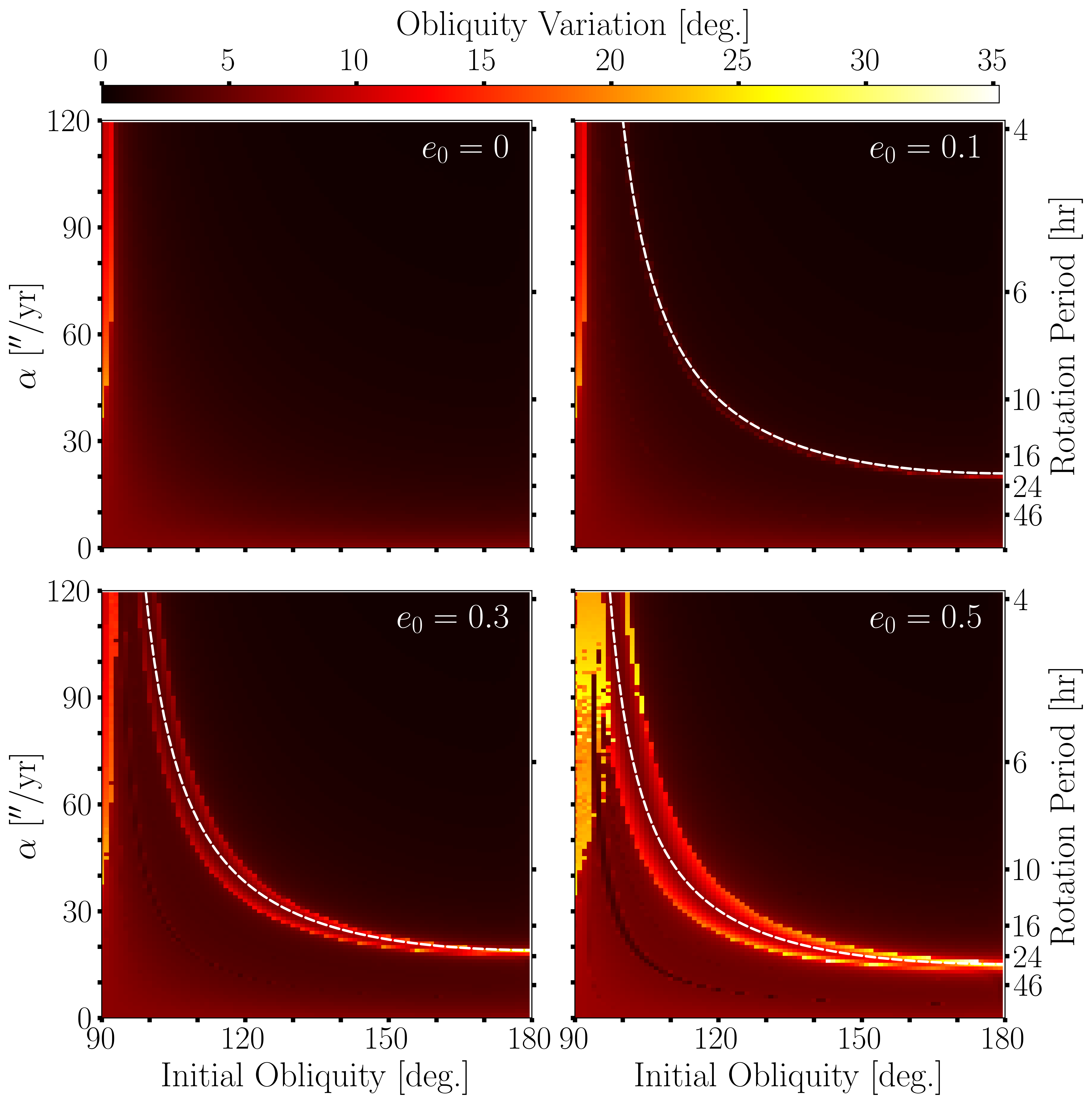
Although we are confident in our methodology and the accuracy of our results, running simulations with SMERCURY is computationally expensive and limits the parameter space that we can explore. We choose to complement our results by examining a broader parameter space and employ the less robust but useful semi-analytical secular spin evolution approach as featured in Quarles et al. 2019. This approach applies a secular time-dependent Hamiltonian to the orbital integration results computed by SMERCURY in order to compute the spin evolution of a planet. We use the same initial conditions as our other simulations (according to Table 1), and apply this model to the 100 Myr, sampled every 100 years, orbital evolution results as featured in Figures 5 and 6. However, we now explore initial obliquities for Earthmoo from to in increments while we sweep the values of the precession constant (relates to rotation period) from 0 ′′/yr to 120 ′′/yr in 1 ′′/yr increments. Here the initial precession angle is .
Looking to Figure 11, we display the range of obliquity variation () each Earthmoo experienced for each case of initial eccentricity. Since we were able to explore a much finer grid of parameter space using this approach, we present our results in different way that more easily highlights the trends. These results are in good agreement with those discussed in Section IV.2. The majority of Earthmoos are quite stable and only vary -, while the cases in which Earthmoo had an initial obliquity near similarly resulted in heightened obliquity variation. The test Earthmoos experienced pronounced obliquity variation near the predicted locations of the spin-orbit resonance. In addition, there is a splitting trend that distinguishes two regimes of variation that follow the predicted resonance location which become more evident for higher values of eccentricity. Figure 12 of Quarles et al. 2020 showcases a similar splitting trend, in which the authors explain that it is a consequence as a result of the difference between the initial precession angle and the initial longitude of ascending node () having a large angular separation from the phase of the resonant orbital frequency (shown as in Table 3). We again find that the magnitude of these variations generally increase with eccentricity (due to increasing amplitudes of the orbital frequencies), where we report a maximum variation of for the Earthmoo with an initial eccentricity of 0.5 with an initial obliquity of and a precession constant of 16 ′′/yr.
IV.4 A Closer Look at the Resonance
Taking the results of our N-body simulations, we can gain additional insight into the nature of this eccentricity-enabled spin-orbit resonance through further analysis. In Section II we discussed that the condition for this resonance was that . The corresponding resonant angle, , is therefore
| (5) |
Saillenfest et al. 2019 provides an analytical theory that identifies this angle as a first-order term that obeys the “Colombo’s Top” Hamiltonian. Here, we use our numerical simulations to verify that is indeed a valid resonant angle, and that it is connected to the observed obliquity variations. We select the Earthmoo with a 16-hour rotation period and an initial obliquity of from the 0.3 initial eccentricity case (featured in Figure 9) to serve as an example. We plot the Earthmoo’s resonant angle and obliquity as functions of time for the first 5 Myr of the simulation in Figure 12. This plot is revealing, and shows that is indeed librating about zero, as one would expect for a valid resonant angle. Furthermore, the variations in lead the variations in obliquity by , implying a direct dynamical connection between these two angles.
The behavior shown in Figure 12 also highlights the importance of initial conditions. Previous work found that the choice of the initial precession angle can influence the obliquity evolution in the sense that it affects the phasing of frequencies involved in the spin-orbit resonance, which in turn moderates the strength of the resonant interactions (Lissauer et al. 2012; Barnes et al. 2016; Quarles et al. 2020). The example Earthmoo in Figure 12 had an initial precession angle of , in which the wide libration of its resonant angle and subsequent large obliquity variations was likely determined by its initial combination of , , and . Therefore we conclude that these angles play a role in controlling the range of affected obliquity configurations near the resonance. Future work could explore this phenomenon.
V Conclusion
We investigate a mechanism in which orbital eccentricity acts to influence the obliquity evolution of retrograde-rotating planets. This mechanism can lead to pronounced obliquity variations in the event of a spin-orbit resonance, when a retrograde rotator’s axial precession frequency becomes commensurate with an eccentricity-enabled orbital frequency. We demonstrate this phenomenon by performing numerical simulations of a toy system consisting of the Sun, a moonless Earth we call Earthmoo, and Jupiter.
We find that the predicted orbital frequency is indeed present for the cases in which Earthmoo is eccentric; this orbital frequency obeys the relationship we describe in Equation 4, while it shifts to higher values and grows in amplitude for greater values of eccentricity. Over the course of the 100 Myr rigid body simulations we find that of the Earthmoos that we test are relatively obliquity stable and experienced variations less than what we expect from orbital variations alone. However, for regions of parameter space near the predicted spin-orbit resonance locations, Earthmoo experienced pronounced obliquity variations of order -. Generally, greater values of eccentricity led to an increase in the fraction of parameter space occupied by solutions with large obliquity variations, in which these variations also increased with increasing eccentricity.
The magnitude of these obliquity variations over this timescale is likely significant in the consideration of habitability. We do not employ a climate model in this work similar to Armstrong et al. 2014, Deitrick et al. 2018b, and others, but others have shown that large swings in a planet’s obliquity could be the deciding factor between conditions that are detrimental to life, or foster it. Although the system that we consider here is purely fictional, we show the importance of the consideration of orbital eccentricity for retrograde-rotating planets and suggest that this effect may be important in future efforts to characterize planetary habitability. Retrograde rotation stabilizes obliquity under most circumstances, but the obliquity evolution of a planet is ultimately at the mercy of its system’s orbital architecture. Retrograde rotators on eccentric orbits can experience high obliquity variability.
Ideally, the knowledge gained by this study and the numerous other obliquity studies could be applied to real exoplanet systems. However, to date, we have not yet been able to directly measure the obliquity of an exoplanet. There are several methodologies that have been proposed to do so, including: constraining obliquity by measuring planetary oblateness and rotation period from transit photometry (Barnes & Fortney 2003), inferring obliquity from seasonal differences in infrared light curves (Gaidos & Williams 2004), obtaining obliquity by looking for geometric effects of directly imaged exoplanets (Kawahara 2016), and others. It is only a matter of time before we gain this capability with future technological advances, where we can then apply our knowledge and make judgements on the habitability of candidate exoplanets based on their obliquity evolution.
VI Acknowledgments
The authors acknowledge support from the NASA Exobiology program, grant #NNX14AK31G. This research was supported in part through research cyberinfrastructure resources and services provided by the Partnership for an Advanced Computing Environment (PACE) at the Georgia Institute of Technology. We thank William J. Miller for his code to produce the nodal precession animation featured in Figure 2a.
VII Orcid iDs
Steven M. Kreyche
https://orcid.org/0000-0002-7274-758X
Jason W. Barnes
https://orcid.org/0000-0002-7755-3530
Billy L. Quarles
https://orcid.org/0000-0002-9644-8330
Jack J. Lissauer
https://orcid.org/0000-0001-6513-1659
Matthew M. Hedman
https://orcid.org/0000-0002-8592-0812
References
- Armstrong et al. (2014) Armstrong, J., Barnes, R., Domagal-Goldman, S., et al. 2014, Astrobiology, 14, 277, pMID: 24611714. https://doi.org/10.1089/ast.2013.1129
- Barnes & Fortney (2003) Barnes, J. W., & Fortney, J. J. 2003, The Astrophysical Journal, 588, 545. https://doi.org/10.1086%2F373893
- Barnes et al. (2016) Barnes, J. W., Quarles, B., Lissauer, J. J., Chambers, J., & Hedman, M. M. 2016, Astrobiology, 16, 487, pMID: 27328026. https://doi.org/10.1089/ast.2015.1427
- Bolmont et al. (2016) Bolmont, E., Libert, A.-S., Leconte, J., & Selsis, F. 2016, A&A, 591, A106. https://doi.org/10.1051/0004-6361/201628073
- Chambers (1999) Chambers, J. E. 1999, Monthly Notices of the Royal Astronomical Society, 304, 793. https://doi.org/10.1046/j.1365-8711.1999.02379.x
- Colose et al. (2019) Colose, C. M., Genio, A. D. D., & Way, M. J. 2019, The Astrophysical Journal, 884, 138. https://doi.org/10.3847%2F1538-4357%2Fab4131
- Deitrick et al. (2018a) Deitrick, R., Barnes, R., Quinn, T. R., et al. 2018a, The Astronomical Journal, 155, 60. https://doi.org/10.3847%2F1538-3881%2Faaa301
- Deitrick et al. (2018b) Deitrick, R., Barnes, R., Bitz, C., et al. 2018b, The Astronomical Journal, 155, 266. https://doi.org/10.3847%2F1538-3881%2Faac214
- Dones & Tremaine (1993) Dones, L., & Tremaine, S. 1993, Icarus, 103, 67
- Dong et al. (2019) Dong, C., Huang, Z., & Lingam, M. 2019, The Astrophysical Journal, 882, L16. https://doi.org/10.3847%2F2041-8213%2Fab372c
- Dressing et al. (2010) Dressing, C. D., Spiegel, D. S., Scharf, C. A., Menou, K., & Raymond, S. N. 2010, The Astrophysical Journal, 721, 1295. https://doi.org/10.1088%2F0004-637x%2F721%2F2%2F1295
- Forget et al. (2013) Forget, F., Wordsworth, R., Millour, E., et al. 2013, Icarus, 222, 81
- Gaidos & Williams (2004) Gaidos, E., & Williams, D. 2004, New Astronomy, 10, 67 . https://doi.org/10.1016/j.newast.2004.04.009
- Guendelman & Kaspi (2019) Guendelman, I., & Kaspi, Y. 2019, The Astrophysical Journal, 881, 67. https://doi.org/10.3847%2F1538-4357%2Fab2a06
- Head et al. (2004) Head, J., Mustard, J., Kreslavsky, M., Milliken, R., & Marchant, D. 2004, Nature, 426, 797
- Head et al. (2005) Head, J. W., Neukum, G., Jaumann, R., et al. 2005, Nature, 434, 346
- Hoffman et al. (1998) Hoffman, P. F., Kaufman, A. J., Halverson, G. P., & Schrag, D. P. 1998, Science, 281, 13421346. https://science.sciencemag.org/content/281/5381/1342
- Hubbard (1984) Hubbard, W. B. 1984, Planetary Interiors (New York, Van Nostrand Reinhold Co.)
- Kane & Torres (2017) Kane, S. R., & Torres, S. M. 2017, The Astronomical Journal, 154, 204. https://doi.org/10.3847%2F1538-3881%2Faa8fce
- Kang (2019) Kang, W. 2019, The Astrophysical Journal, 876, L1. https://doi.org/10.3847%2F2041-8213%2Fab18a8
- Kawahara (2016) Kawahara, H. 2016, The Astrophysical Journal, 822, 112. https://doi.org/10.3847%2F0004-637x%2F822%2F2%2F112
- Kilic et al. (2018) Kilic, C., Lunkeit, F., Raible, C. C., & Stocker, T. F. 2018, The Astrophysical Journal, 864, 106. https://doi.org/10.3847%2F1538-4357%2Faad5eb
- Kilic et al. (2017) Kilic, C., Raible, C. C., & Stocker, T. F. 2017, The Astrophysical Journal, 844, 147. https://doi.org/10.3847%2F1538-4357%2Faa7a03
- Laskar et al. (1993a) Laskar, J., Joutel, F., & Boudin, F. 1993a, A&A, 270, 522. https://ui.adsabs.harvard.edu/abs/1993A&A...270..522L
- Laskar & Robutel (1993b) Laskar, J., & Robutel, P. 1993b, Nature, 361, 608. https://doi.org/10.1038/361608a0
- Li & Batygin (2014) Li, G., & Batygin, K. 2014, The Astrophysical Journal, 790, 69. https://doi.org/10.1088%2F0004-637x%2F790%2F1%2F69
- Lissauer et al. (2012) Lissauer, J. J., Barnes, J. W., & Chambers, J. E. 2012, Icarus, 217, 77 . https://doi.org/10.1016/j.icarus.2011.10.013
- Lissauer et al. (1997) Lissauer, J. J., Berman, A. F., Greenzweig, Y., & Kary, D. M. 1997, Icarus, 127, 65
- Lissauer & Kary (1991) Lissauer, J. J., & Kary, D. M. 1991, Icarus, 94, 126 . http://www.sciencedirect.com/science/article/pii/001910359190145J
- Méndez & Rivera-Valentín (2017) Méndez, A., & Rivera-Valentín, E. G. 2017, The Astrophysical Journal, 837, L1. https://doi.org/10.3847%2F2041-8213%2Faa5f13
- Miguel & Brunini (2010) Miguel, Y., & Brunini, A. 2010, Monthly Notices of the Royal Astronomical Society, 406, 1935. https://doi.org/10.1111/j.1365-2966.2010.16804.x
- Milanković (1998) Milanković, M. 1998, Canon of Insolation and the Ice-Age Problem [translation] (Zavod za Udžbenike i Nastavna Sredstva)
- Millholland & Batygin (2019) Millholland, S., & Batygin, K. 2019, The Astrophysical Journal, 876, 119. https://doi.org/10.3847%2F1538-4357%2Fab19be
- Muller & MacDonald (1995) Muller, R. A., & MacDonald, G. J. 1995, Nature, 377, 107
- Murray & Dermott (1999) Murray, C. D., & Dermott, S. F. 1999, Solar System Dynamics (Cambridge University Press)
- Neron de Surgy & Laskar (1997) Neron de Surgy, O., & Laskar, J. 1997, A&A, 318, 975
- Olson et al. (2019) Olson, S. L., Jansen, M., & Abbot, D. S. 2019, arXiv e-prints, arXiv:1909.02928
- Quarles et al. (2020) Quarles, B., Barnes, J. W., Lissauer, J. J., & Chambers, J. 2020, Astrobiology, 20, 73, pMID: 31613645. https://doi.org/10.1089/ast.2018.1932
- Quarles et al. (2019) Quarles, B., Li, G., & Lissauer, J. J. 2019, The Astrophysical Journal, 886, 56. https://doi.org/10.3847%2F1538-4357%2Fab46b5
- Saillenfest et al. (2019) Saillenfest, M., Laskar, J., & Boué, G. 2019, A&A, 623, A4. https://doi.org/10.1051/0004-6361/201834344
- Šidlichovský & Nesvorný (1996) Šidlichovský, M., & Nesvorný, D. 1996, Celestrial Mechanics and Dynamical Astronomy, 65, 137. https://doi.org/10.1007/BF00048443
- Spiegl et al. (2015) Spiegl, T., Paeth, H., & Frimmel, H. 2015, Earth and Planetary Science Letters, 415, 100. https://doi.org/10.1016/j.epsl.2015.01.035
- van den Heuvel (1966) van den Heuvel, E. P. J. 1966, Geophysical Journal International, 11, 323. https://doi.org/10.1111/j.1365-246X.1966.tb03086.x
- Way & Georgakarakos (2017) Way, M. J., & Georgakarakos, N. 2017, The Astrophysical Journal, 835, L1. https://doi.org/10.3847%2F2041-8213%2F835%2F1%2Fl1
- Williams & Kasting (1997) Williams, D. M., & Kasting, J. F. 1997, Icarus, 129, 254. https://doi.org/10.1006/icar.1997.5759
- Williams & Pollard (2002) Williams, D. M., & Pollard, D. 2002, International Journal of Astrobiology, 1, 61. https://doi.org/10.1017/S1473550402001064
- Williams & Pollard (2003) —. 2003, International Journal of Astrobiology, 2, 1. https://doi.org/10.1017/S1473550403001356