Learning Theory for Estimation of
Animal Motion Submanifolds
Abstract
This paper describes the formulation and experimental testing of a method to estimate submanifold models of animal motion. It is assumed that the animal motion is supported on a configuration manifold, , and that the manifold is homeomorphic to a known smooth, Riemannian manifold, . Estimation of the configuration submanifold is achieved by approximating an unknown mapping, , from to . The overall problem is cast as a distribution-free learning problem over the manifold of measurements. This paper introduces linear approximation spaces in that contain approximations of corresponding to those known for classical distribution-free learning theory over Euclidean space. This paper concludes with a study and discussion of the performance of the proposed method using samples from recent reptile motion studies.
I Introduction
The related problems of understanding the underlying dynamics of animal locomotion, constructing (multibody) dynamics models of animals, or building robots that emulate animals have occupied researchers having diverse backgrounds. Research in [1, 2, 3, 4, 5] includes investigations related to, or based upon, the motions of humans, bats, birds, lizards, geckos, sheep, frogs, beetles, and cheetahs. Some studies such as in [6, 7, 8, 9] seek to understand and utilize the underlying geometry of the mechanics of human or other animal motion. Others are expressly interested in the construction of low dimensional models of complex motion [10, 11, 12]. Some are dedicated to finding how qualitative understandings of animal motion can be used to build robots that emulate some observed motion [13, 14, 15, 16, 17], with a notable emphasis on locomotion in quadrupeds [18, 19, 20, 21, 22] and bipeds [23, 24, 25, 26, 27, 28].
A fundamental question that is either motivated or directly addressed by these studies is how to come up with a general method for defining a principled, low-dimensional model of a complex animal motion. None of the aforementioned references describe or derive a general strategy that is applicable, in principle, across a broad range of animal motion studies. Just as importantly, none of the references establish rates of convergence that would give confidence in estimates of such low dimensional systems. The aim of our research is to provide further insight into the motion of animals by deriving such a general method to discover and approximate an underlying manifold on which the dynamics evolves.
The theory that has been used to derive models of animal motion has been around for some time. These include general multibody dynamics formulations like [29], or the more recent geometric methods [30, 31]. As discussed carefully in [31], one of the primary theoretical advantages of geometric methods is their abstraction: states of the system are known to be elements of manifolds, which are by their nature coordinate-free. This generality is particularly attractive in the problem at hand. Intuitively, we want to approximate or identify some “lower-dimensional mathematical object” that underlies an observed motion of a complex, higher order multibody system. We want to ensure that any associated algorithm converges to a coordinate independent entity. In this paper we introduce the analysis and experimental testing of a method to identify and approximate motions over a submanifold that underlies a particular motion regime observed during animal motion. We work to formulate the problem in such a way that we can guarantee that approximations converge, in some appropriate sense, over the underlying manifold.
We begin in Section II-B with a careful description of the problem of estimating a motion manifold as one of distribution-free learning over manifolds. This problem is substantially more complicated than the conventional problems for functions defined over Euclidean spaces. This new learning problem is made complex in no small part owing to the difficulty of defining appropriate function spaces and spaces of approximants over manifolds. These two topics are covered in Sections II-C and II-D, respectively. In particular, we introduce the linear approximation spaces for a smooth manifold , and these play a crucial role in deriving rates of convergence. The primary theoretical result of this paper gives sufficient conditions to ensure that approximations of the unknown function converge to the regressor function . Additionally, we show that when the regressor function satisfies the smoothness condition , the rate of convergence is given by
| (1) |
for constants , where is the expectation over samples, is the dimension of the space of approximants, and is the number of samples. This is precisely the rate achieved for certain approximations of distribution-free learning problems over Euclidean space. Such rates of convergence are known to be optimal in the Euclidean case, except for the logarithmic factor. [32] Finally, this paper concludes in Section III with a study of the performance of the proposed method using samples from recent reptile motion studies.
II Problem Formulation
II-A Kinematics and Inherent Geometry
For purposes of ensuring convergence of approximations, we assume in this paper that motions are supported on a configuration manifold, , that is contained in the ambient space for some . Of course this space suffices to describe the dynamics of multibody systems comprised of assemblies of lumped masses where motion is specified in terms of the mass centers of the (inertia-free) bodies. Since any Riemannian manifold can be (isometrically) embedded in for a large enough via the Nash embedding theorem, in principle this assumption also allows for some of the other standard models where the configuration manifold includes SO(3) or SE(3) as described in [31, 30]. It is further assumed that the manifold is a smooth, compact, connected, Riemannian manifold that is regularly embedded in the ambient space This manifold is taken to be homeomorphic to some known smooth manifold . We denote the homeomorphism by where and , and we discuss its smoothness in our discussion of approximation spaces in Section II-C. The manifold is equipped with the topology induced by its intrinsic Riemannian metric and is equipped with the topology inherited as a regularly embedded submanifold .
II-B The Distribution-Free Learning Problem on Manifolds
This paper is concerned with finding or approximating the mapping that determines the low-dimensional underlying manifold that supports a given motion or motion regime. We choose to formulate this problem as one of distribution-free learning theory on manifolds. In distribution-free learning theory it is assumed that we are given a collection of independent and identically distributed samples that that are generated by some unknown probability measure on the manifold . In order to determine the mapping from the known manifold to the configuration space , it would be ideal if we could determine an optimal mapping such that
| (2) |
where and is a set of admissible operators that map from . Solving the optimization problem 2 poses a number of difficulties, some of which are rather standard challenges in the field of distribution-free learning theory. For example, it is well-known that the ideal solution above cannot be computed from the minimization problem in Equation 2 since the measure on is unknown. For this reason methods of empirical risk minimization are used that substitute a discrete proxy for the expression in Equation 2. We discuss this step in detail shortly in Section II-E.
Beyond these conventional challenges to building approximations of , there are additional substantial difficulties that are unique to the problem at hand. In classical treatments of distribution-free learning theory, the rates of convergence of approximations to the solution are often cast in terms of approximation spaces or smoothness spaces (that often end up being Sobolev spaces) of real-valued functions over subsets of Euclidean space . That is, the space is usually selected to be some subset of the real-valued functions over subsets of Euclidean space. Here, however, the functions are mappings from the manifold to the manifold . The definition of Sobolev mappings between manifolds is a complicated subject, and for general choices of or it is unclear exactly what definition of smoothness should be selected. A significant part of this paper is dedicated to defining approximation spaces, , over manifolds to characterize smoothness or approximation properties and subsequently structuring the learning problem so convergence results can be derived in a way that is analogous to the classical case over subsets of Euclidean Space.
II-C Function Spaces on Manifolds
In the setup of the problem above we have assumed that is a known, compact, connected, smooth Riemannian manifold, and that is a regularly embedded submanifold of . This means that the unknown function is constructed of component functions for . In this section we define the various function spaces over manifolds that will be used to approximate the functions . The function spaces over the manifold that is used in this paper consist of certain spaces of square-integrable functions and native spaces of a reproducing kernel. When is a measure over the manifold , the usual space of real-valued, -square integrable functions is given by , which is a Hilbert space with respect to the usual inner product . Recall [33, 34] that a real RKH space over an arbitrary set is defined to be where and is a real, positive semi-definite, symmetric, continuous admissible kernel function. This definition of an RKH space makes sense over a general set , and in particular makes sense for the specification of functions over manifolds. We denote by the kernel of the RKH Space over the set . The restriction of functions in to the set always defines an RKH space over , and we set . The kernel that defines the space of restrictions is given by , for all , which is a classical result from the theory of RKH spaces. Finally, we define the pullback space on as and the kernel defined on the manifold is written as
II-D Approximant Spaces
The approximations in this paper are constructed in terms of two different types of finite dimensional spaces of approximants.
II-D1 Approximants in
When we build approximations in , we make use of a nested sequence of measurable partitions of , where each partition . That is, these sets satisfy , for all , and for some finite set of indices . Here is the number of sets in the partition . We define the space of approximants as the span of the characteristic functions of the sets in , where is the associated partition of unity over . We associate to the partition a set of representatives, These representative points are assumed to fill the manifold in the sense that the fill distance as . For any we define the -orthogonal projection in the usual way,
We define the linear approximation space of functions defined over the manifold as
The infimum of the constants , for which in the inequality above holds, defines a semi-norm on . We note that if is a compact subset of Euclidean space and is a Lebesgue measure, these spaces can be understood in some cases as Sobolev spaces [32]. Here the expression above defines approximation spaces over the manifold .
II-D2 Approximants in
II-E Empirical Risk Minimization over Manifolds
As noted above, in some ideal sense the optimal choice of the mapping is the one that extremizes the cost functional in Equation 2. Since the measure that generates the samples in is unknown, distribution-free learning theory uses a proxy that can be computed to re-cast the optimization problem. The form of the empirical risk can best be motivated by first rewriting the ideal risk in terms of the regressor function. Any measure on the space of samples can be rewritten (disintegrated) into the expression with , the associated marginal measure over , and the conditional probability measure on given . From first principles it is straightforward to show that we can rewrite the ideal cost in the alternative form
| (3) |
where is the regressor function associated with the measure . This decomposition shows, in fact, that the optimal mapping that minimizes is the regressor function . Since the last term on the right in Equation 3 is a constant that does not depend on , we introduce the empirical risk
| (4) |
in terms of the samples . Note that the cost functional can be computed for any admissible function since the samples are known. We will be interested in two types of approximations of the empirical risk in the discussions that follow. We define
| (5) |
when we seek approximations that converge in . This definition has the advantage that it is possible to derive strong convergence rates for the approximations . However, the resulting approximations are not very smooth. Alternatively, we replace by in Equation 5 when we seek smoother representations of the mapping . As of yet, we have not derived such strong rates of convergence in this case. However, numerical examples compare the performance of the estimates obtained with the choices and .
Before we study the solutions of these distribution-free learning problems over the manifold , we make one last observation regarding the form of minimization problem. By introducing the samples and mapping , we can write
with . Note that since each term is positive, the optimal can be obtained by extremizing each of the terms for the component functions for . The primary theoretical result of this paper is summarized in the following theorem, which solves the distribution free learning problem over manifold
Theorem 1
The optimal solution of the empirical risk minimization problem in Equation 4 is given by
If the regressor , we have the error bound
| (6) |
where the constant is independent of and and is the expectation on with the product measure .
Proof:
When we define , we have the explicit representation of given by
We can also write this sum as
and this summation can be reordered as and
with each depending on a single variable . By taking the partial derivative , we see that which establishes the form of solution stated above. We now turn to the consideration of the error bound in the theorem. From the triangle inequality
we can bound the first term above by from the definition of the linear approximation space . The bound in the theorem is proven if we can show that there is a constant such that . We establish this bound by a straightforward extension to functions on the manifold of the proof in [37], which is given for functions defined on for . The expression above for can be written in the form , and that for can be written as . In terms of these expansions, we write the error as ∥ Π^S_n γ^j_μ-γ_n,m∥^2_L^2_μ(S)=∑_k=1^N(n) ( α_n,k^j- ^ α _n,k^j )^2μ_S(S_n,k). Let be an arbitrary, but fixed, positive number. We define the set of indices that denote subsets that have, in a sense, small measure,
where is . We define the complement , and then set the associated sums and . The bound in Equation 1 follows if we can demonstrate a concentration of measure formula
| (7) | ||||
for some constants . See [37, 32] for a discussion of such concentration inequalities. The fact that such a concentration inequality implies the bound in expectation in Equation 1 is proven in [37] on page 1311 for functions over Euclidean space. The argument proceeds exactly in the same way for the problem at hand by integration of the distribution function defined by Equation 7 over the manifold . To establish the concentration inequality, let us define two events , and We can compute directly from the definitions of the coefficients , and using the the compactness of , that for any . Since we always have
is bounded below by , we know that for any . If the inequality , then we know there is at least one such that
When we define the event for each , we conclude By the monotonicity of measures, we conclude that . But we can show, again by a simple modification of the arguments on page of [37], that . The analysis proceeds as in that reference by using Bernstein’s inequality for random variables defined over the probability space instead of over Euclidean space.
∎
III Experiments and Numerical Examples
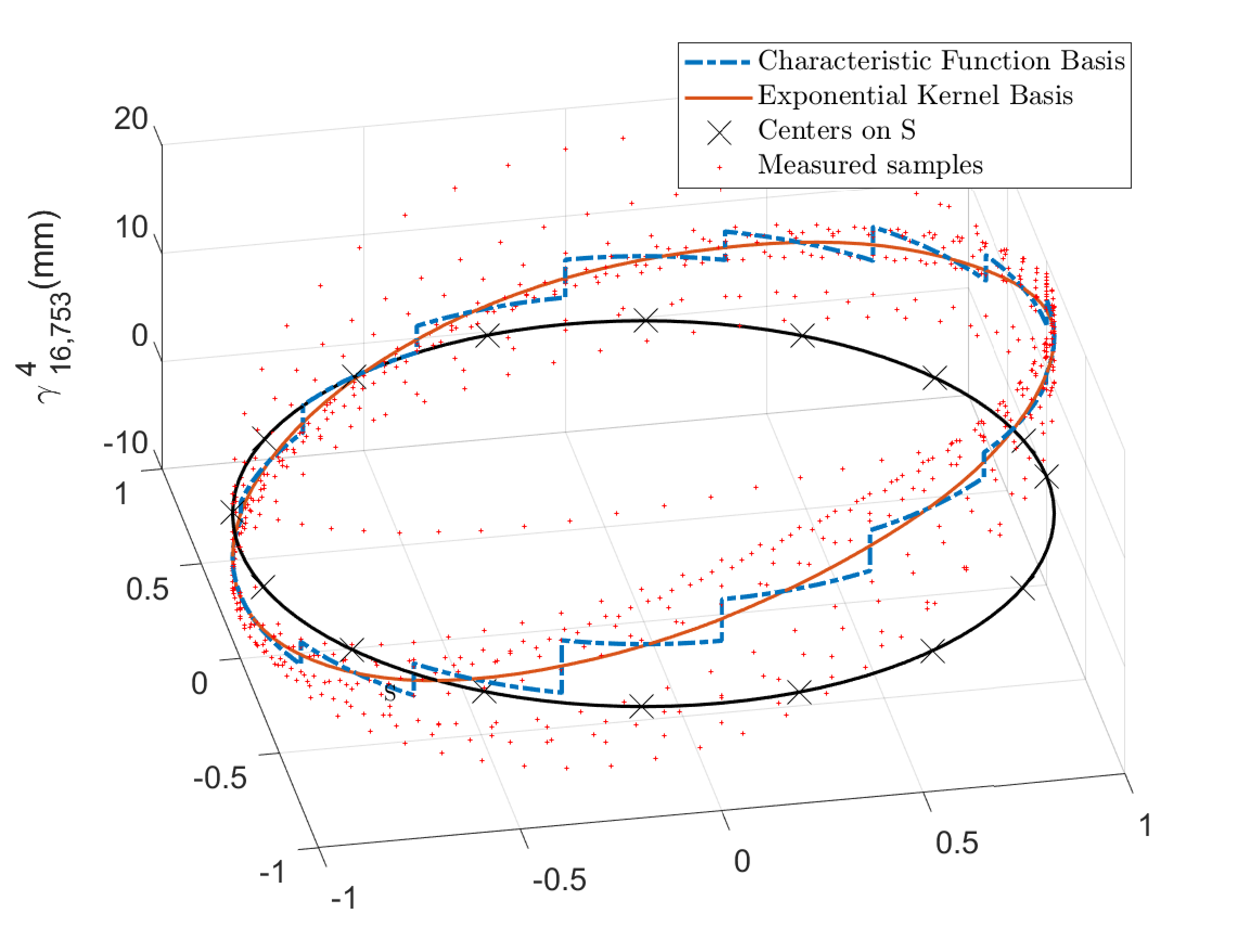
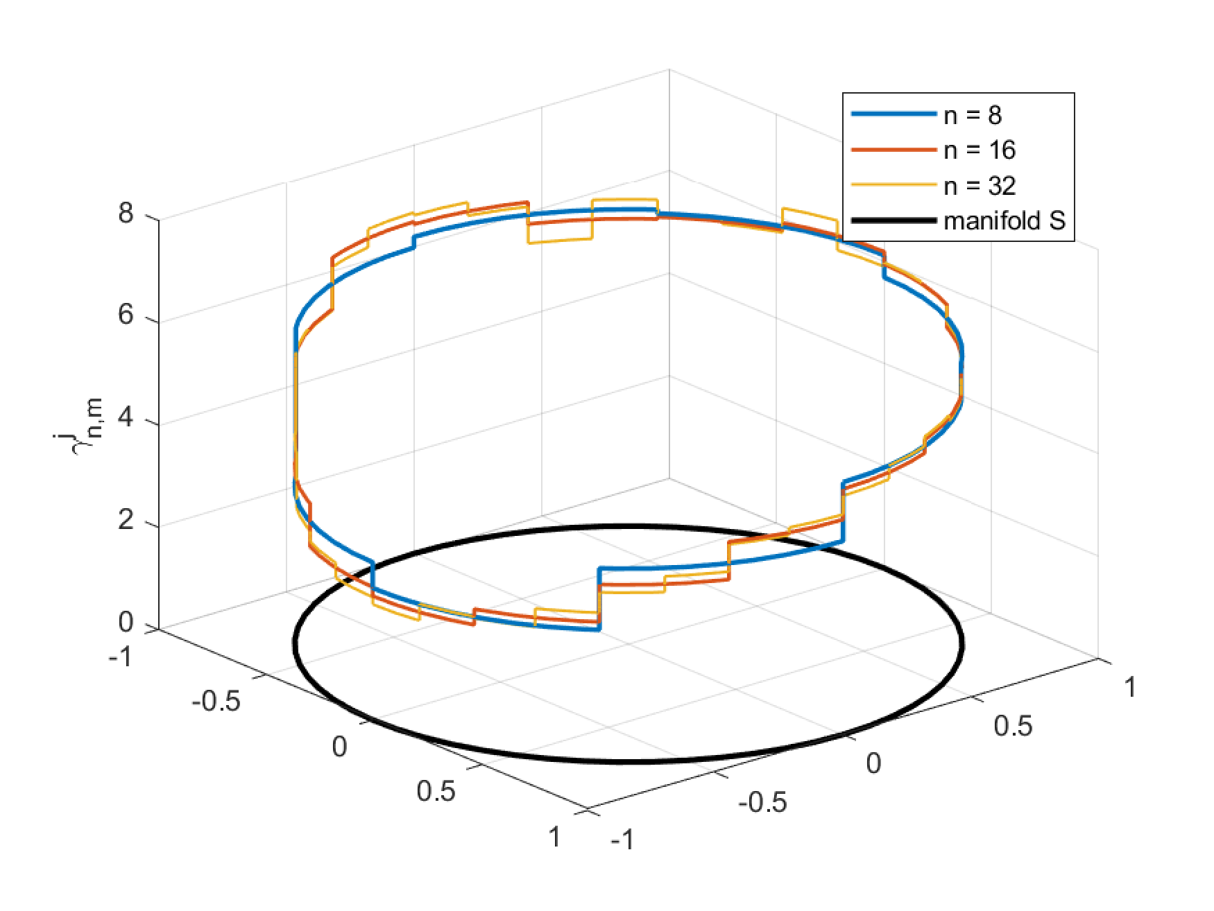
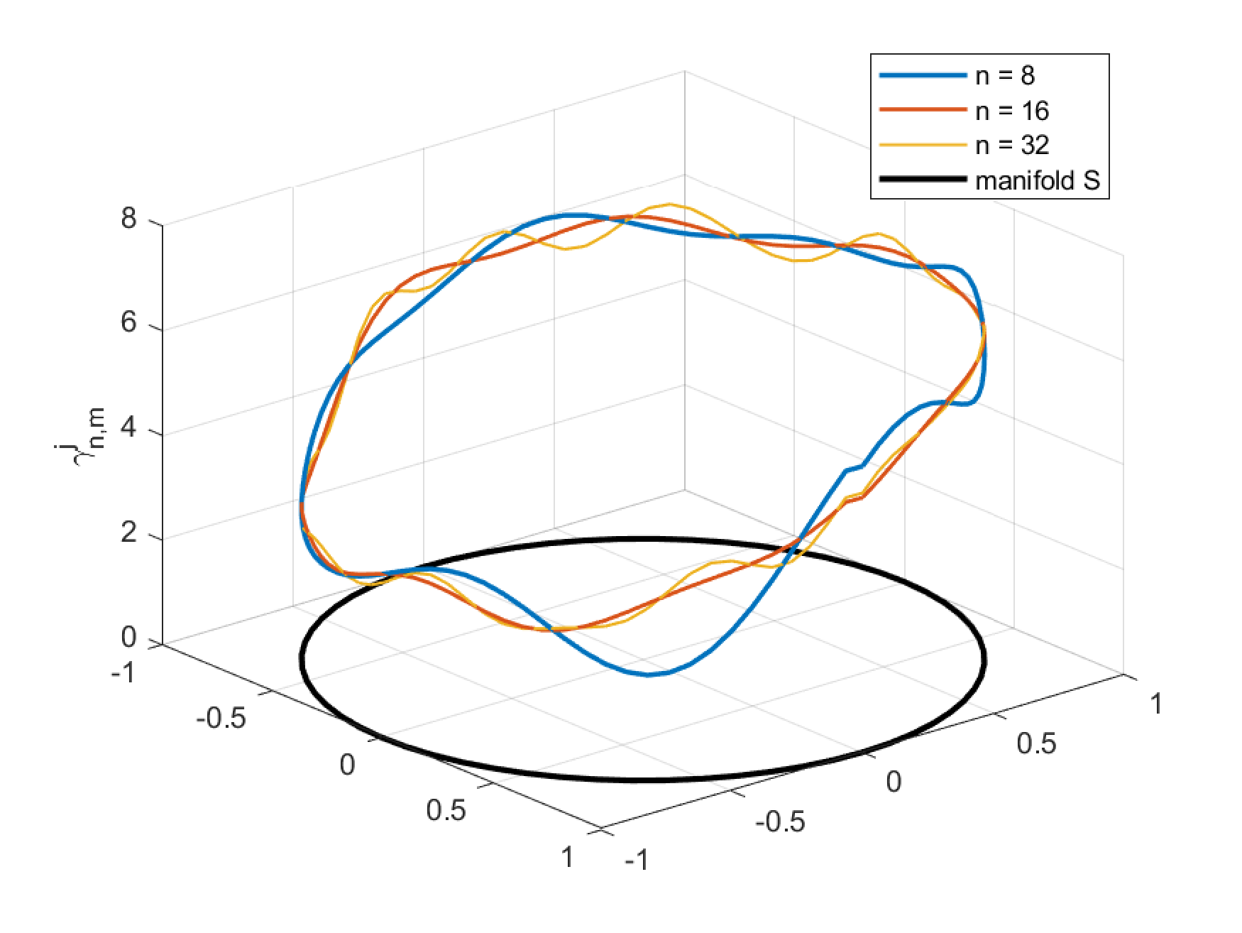
A number of experiments and simulations have been carried out to study the performance of the analysis in the paper. Photoreflective markers were placed on specimens of anolis sagrei as depicted in Figure 1, which then traversed an inclined, narrow board within the line of sight of three high speed, Photron FASTCAM ®cameras. Video imagery was recorded at 500 fps, and inertial trajectories such as those depicted in Figure 2 of the markers were estimated using the publicly distributed software toolbox [38]. The discrete inertial trajectories are interpreted as measured samples . In this example, we hypthesize that the observed configuration space is homeomorphic to a one-dimensional, compact space. Consequently, we choose the known manifold , the circle in , and we seek a mapping where is the unknown manifold homeomorphic to . The approximation is obtained as the solution of the empirical risk minimization problem for two choices and of approximant subspaces in the plots that follow. The basis for is taken to be given by translates of the exponential kernel . Figures 3 and 4 compare the performance of the two methods of approximation as the number of samples and the dimension of the approximation spaces are varied.
Figure 4 illustrates the effects that the number of centers has on the fidelity of the approximation. For both methods, it is clear that increasing the dimension number of partitions corresponds to a higher resolution that manages to capture changes in the data over smaller intervals. The EDMD approximations generated from the exponential kernel are also dependent on the hyperparameter .


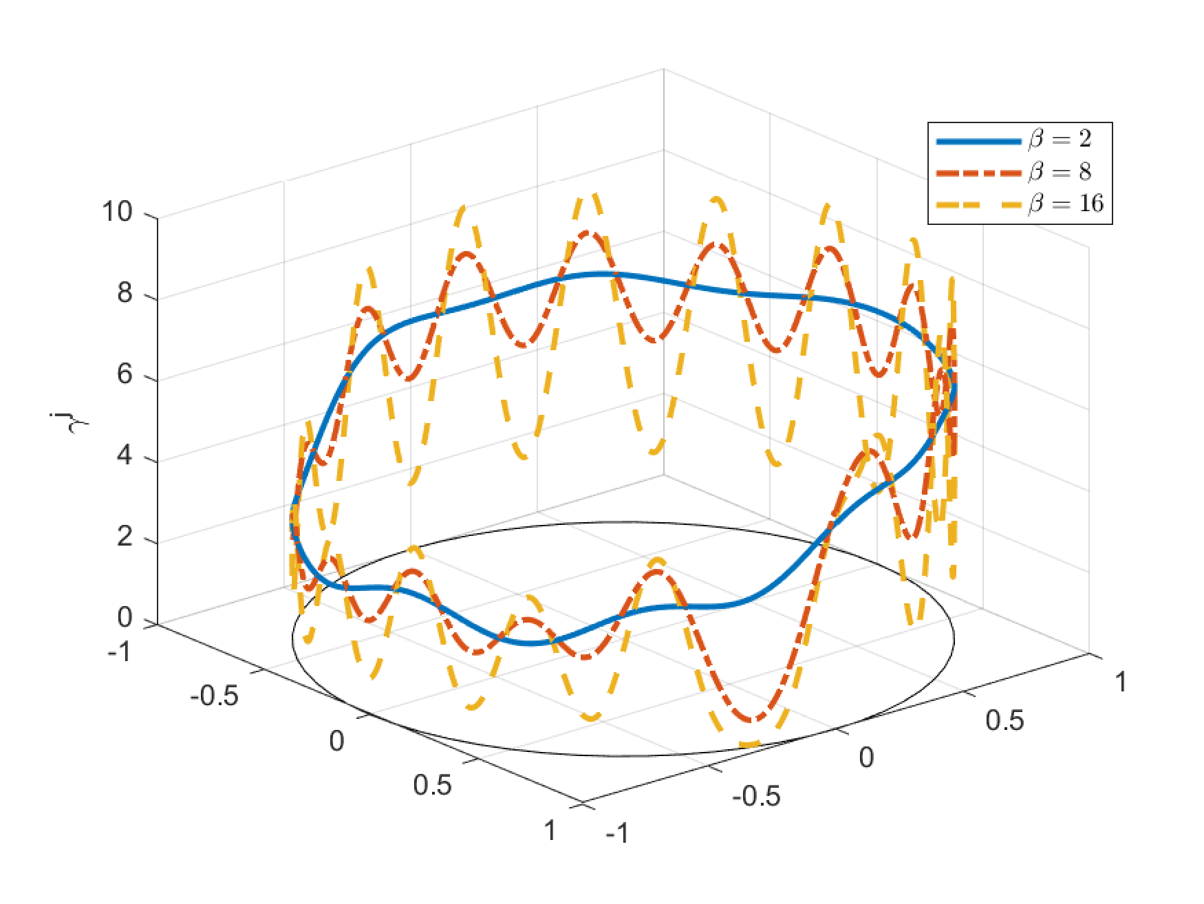
Figure 5 illustrates the effects of the hyperparameter on the approximation. For an exponential basis, larger values of result in basis functions that decay rapidly from their centers, "sharpening" the curve. This results in a more oscillatory approximation from the basis functions. Thus,while the optimization of the empirical risk for functions in yields nonsmooth estimates, there is no analog to the hyperparameter . Depending on the hyperparameter , highly oscillatory solutions can result for different choices of , even for EDMD solutions over approximant spaces having the same dimension . Such oscillations can be addressed in the EDMD methods or Gaussian process models by introducing a regularization parameter. [35]
IV Conclusions
This study has derived a general formulation of the problem to approximate a submanifold representing animal motion from observations. The general form of the problem has been stated as a type of distribution-free learning over a smooth manifold. The paper defines a closed form expression for approximations of the map that defines the manifold, and derives bounds for the rates of convergence over the manifold that are analogous to those obtained in corresponding problems over Euclidean spaces.
Appendix
Let the sample pairs be deonted . Where . By definition
We also know that ) ( is assumed to be bijective)
By definition and
Suppose that
We know that the operator interpolates over and that this interpolant is unique. interpolates over which is mapped to which once again interpolates over . Therefore the following equality holds.
How to express the . We know that
Denote
Recall that
| (8) |
IV-A Element-wise Homogenization
Where
IV-B Aggregation
Let
Then
Define
Where is the Lagrange basis for .
Then we have
So . Let be a partition of . . . on
The set is and
Let . is the Lagrange basis associated with .
By definition .
Recall
Define
Then
And
Now look at
References
- [1] Matt J. Bender, Mark McClelland, Gerardo Bledt, Andrew Kurdila, Tomonari Furukawa, and Rolf Mueller. Trajectory Estimation of Bat Flight Using a Multi-View Camera System. AIAA Modeling and Simulation Technologies Conference, (January):1–13, 2015.
- [2] Aleksandra V. Birn-Jeffery and Timothy E. Higham. Geckos decouple fore- and hind limb kinematics in response to changes in incline. Frontiers in Zoology, 13(1):1–13, 2016.
- [3] Penny E Hudson, Sandra A Corr, and Alan M Wilson. High speed galloping in the cheetah (acinonyx jubatus) and the racing greyhound (canis familiaris): spatio-temporal and kinetic characteristics. Journal of Experimental Biology, 215(14):2425–2434, 2012.
- [4] Rivers Ingersoll, Lukas Haizmann, and David Lentink. Biomechanics of hover performance in Neotropical hummingbirds versus bats. Science Advances, 4(9), 2018.
- [5] Laura B Porro, Amber J Collings, Enrico A Eberhard, Kyle P Chadwick, and Christopher T Richards. Inverse dynamic modelling of jumping in the red-legged running frog, kassina maculata. Journal of Experimental Biology, 220(10):1882–1893, 2017.
- [6] Stanislas Brossette, Adrien Escande, and Abderrahmane Kheddar. Multicontact Postures Computation on Manifolds. IEEE Transactions on Robotics, 34(5):1252–1265, 2018.
- [7] Josip Ćesić, Vladimir Joukov, Ivan Petrović, and Dana Kulić. Full body human motion estimation on lie groups using 3D marker position measurements. IEEE-RAS International Conference on Humanoid Robots, pages 826–833, 2016.
- [8] Ross L Hatton and Howie Choset. Nonconservativity and noncommutativity in locomotion. The European Physical Journal Special Topics, 224(17-18):3141–3174, 2015.
- [9] Elie A. Shammas, Howie Choset, and Alfred A. Rizzi. Geometric motion planning analysis for two classes of underactuated mechanical systems. International Journal of Robotics Research, 26(10):1043–1073, 2007.
- [10] Matt Bender, Xu Yang, Hui Chen, Andrew Kurdila, and Rolf Müller. Gaussian process dynamic modeling of bat flapping flight. In 2017 IEEE International Conference on Image Processing (ICIP), pages 4542–4546, 2017.
- [11] Jennifer M Rieser, Chaohui Gong, Henry C Astley, Perrin E Schiebel, Ross L Hatton, Howie Choset, and Daniel I Goldman. Geometric phase and dimensionality reduction in locomoting living systems. arXiv preprint arXiv:1906.11374, 2019.
- [12] Jack M Wang, David J Fleet, and Aaron Hertzmann. Gaussian process dynamical models for human motion. IEEE transactions on pattern analysis and machine intelligence, 30(2):283–298, 2007.
- [13] J Bayandor, G Bledt, Shirin Dadashi, Andrew Kurdila, I Murphy, and Yu Lei. Adaptive control for bioinspired flapping wing robots. In 2013 American Control Conference, pages 609–614. IEEE, 2013.
- [14] Tomislav Horvat, Kamilo Melo, and Auke J Ijspeert. Spine controller for a sprawling posture robot. IEEE Robotics and Automation Letters, 2(2):1195–1202, 2017.
- [15] Konstantinos Karakasiliotis, Robin Thandiackal, Kamilo Melo, Tomislav Horvat, Navid K Mahabadi, Stanislav Tsitkov, Jean-Marie Cabelguen, and Auke J Ijspeert. From cineradiography to biorobots: an approach for designing robots to emulate and study animal locomotion. Journal of The Royal Society Interface, 13(119):20151089, 2016.
- [16] Qing Shi, Chang Li, Kang Li, Qiang Huang, Hiroyuki Ishii, Atsuo Takanishi, and Toshio Fukuda. A modified robotic rat to study rat-like pitch and yaw movements. IEEE/ASME Transactions on Mechatronics, 23(5):2448–2458, 2018.
- [17] Tien Van Truong, Tuyen Quang Le, Doyoung Byun, Hoon Choel Park, and Minjun Kim. Flexible Wing Kinematics of a Free-Flying Beetle (Rhinoceros Beetle Trypoxylus Dichotomus). Journal of Bionic Engineering, 9(2):177–184, 2012.
- [18] Yibin Li, Bin Li, Jiuhong Ruan, and Xuewen Rong. Research of mammal bionic quadruped robots: A review. In 2011 IEEE 5th International Conference on Robotics, Automation and Mechatronics (RAM), pages 166–171. IEEE, 2011.
- [19] Sangok Seok, Albert Wang, Meng Yee Chuah, David Otten, Jeffrey Lang, and Sangbae Kim. Design principles for highly efficient quadrupeds and implementation on the mit cheetah robot. In 2013 IEEE International Conference on Robotics and Automation, pages 3307–3312. IEEE, 2013.
- [20] Claudio Semini, Victor Barasuol, Jake Goldsmith, Marco Frigerio, Michele Focchi, Yifu Gao, and Darwin G Caldwell. Design of the hydraulically actuated, torque-controlled quadruped robot hyq2max. IEEE/ASME Transactions on Mechatronics, 22(2):635–646, 2016.
- [21] Marc Raibert. BigDog, the rough-terrain quadruped robot. IFAC Proceedings Volumes (IFAC-PapersOnline), 17(1 PART 1):6–9, 2008.
- [22] Barkan Ugurlu, Ioannis Havoutis, Claudio Semini, and Darwin G Caldwell. Dynamic trot-walking with the hydraulic quadruped robot—hyq: Analytical trajectory generation and active compliance control. In 2013 IEEE/RSJ International Conference on Intelligent Robots and Systems, pages 6044–6051. IEEE, 2013.
- [23] Steven H Collins and Andy Ruina. A bipedal walking robot with efficient and human-like gait. In Proceedings of the 2005 IEEE international conference on robotics and automation, pages 1983–1988. IEEE, 2005.
- [24] Twan Koolen, Sylvain Bertrand, Gray Thomas, Tomas De Boer, Tingfan Wu, Jesper Smith, Johannes Englsberger, and Jerry Pratt. Design of a momentum-based control framework and application to the humanoid robot atlas. International Journal of Humanoid Robotics, 13(01):1650007, 2016.
- [25] Francesca Negrello, Manolo Garabini, Manuel G Catalano, Przemyslaw Kryczka, Wooseok Choi, Darwin G Caldwell, Antonio Bicchi, and Nikolaos G Tsagarakis. Walk-man humanoid lower body design optimization for enhanced physical performance. In 2016 IEEE International Conference on Robotics and Automation (ICRA), pages 1817–1824. IEEE, 2016.
- [26] Christian Ott, Maximo A Roa, and Gerd Hirzinger. Posture and balance control for biped robots based on contact force optimization. In 2011 11th IEEE-RAS International Conference on Humanoid Robots, pages 26–33. IEEE, 2011.
- [27] Nicolaus A Radford, Philip Strawser, Kimberly Hambuchen, Joshua S Mehling, William K Verdeyen, A Stuart Donnan, James Holley, Jairo Sanchez, Vienny Nguyen, Lyndon Bridgwater, et al. Valkyrie: Nasa’s first bipedal humanoid robot. Journal of Field Robotics, 32(3):397–419, 2015.
- [28] Benjamin J Stephens and Christopher G Atkeson. Dynamic balance force control for compliant humanoid robots. In 2010 IEEE/RSJ international conference on intelligent robots and systems, pages 1248–1255. IEEE, 2010.
- [29] Ahmed Shabana. Dynamics of multibody systems. Cambridge university press, 2020.
- [30] Kevin M Lynch and Frank C Park. Modern Robotics. Cambridge University Press, 2017.
- [31] Francesco Bullo and Andrew D. Lewis. Geometric Control of Mechanical Systems, volume 49 of Texts in Applied Mathematics. Springer Verlag, New York-Heidelberg-Berlin, 2004.
- [32] Ronald DeVore, Gerard Kerkyacharian, Dominique Picard, and Vladimir Temlyakov. Approximation methods for supervised learning. Foundations of Computational Mathematics, 6(1):3–58, 2006.
- [33] Saburou Saitoh, Daniel Alpay, Joseph A Ball, and Takeo Ohsawa. Reproducing Kernels and Their Applications, volume 3. Springer Science & Business Media, 2013.
- [34] Alain Berlinet and Christine Thomas-Agnan. Reproducing kernel Hilbert spaces in probability and statistics. Springer Science & Business Media, 2011.
- [35] Stefan Klus, Ingmar Schuster, and Krikamol Muandet. Eigendecompositions of transfer operators in reproducing kernel hilbert spaces. Nonlinear Science, 30:283–315, 2020.
- [36] Steven L Brunton and J Nathan Kutz. Data-driven science and engineering: Machine learning, dynamical systems, and control. Cambridge University Press, 2019.
- [37] Peter Binev, Albert Cohen, Wolfgang Dahmen, Ronald DeVore, and Vladimir Temlyakov. Universal algorithms for learning theory part i: piecewise constant functions. Journal of Machine Learning Research, 6(Sep):1297–1321, 2005.
- [38] Tyson L Hedrick. Software techniques for two-and three-dimensional kinematic measurements of biological and biomimetic systems. Bioinspiration & biomimetics, 3(3):034001, 2008.