Generating Weakly Chordal Graphs from Arbitrary Graphs
Abstract
We propose a scheme for generating a weakly chordal graph from a randomly generated input graph, . We reduce to a chordal graph by adding fill-edges, using the minimum vertex degree heuristic. Since is necessarily a weakly chordal graph, we use an algorithm for deleting edges from a weakly chordal graph that preserves the weak chordality property of . The edges that are candidates for deletion are the fill-edges that were inserted into . In order to delete a maximal number of fill-edges, we maintain these in a queue. A fill-edge is removed from the front of the queue, which we then try to delete from . If this violates the weak chordality property of , we reinsert this edge at the back of the queue. This loop continues till no more fill-edges can be removed from . Operationally, we implement this by defining a deletion round as one in which the edge at the back of the queue is at the front. We stop when the size of the queue does not change over two successive deletion rounds and output .
1 Introduction
A graph is said to be weakly chordal if neither nor its complement, , has an induced chordless
cycle on five or more vertices (a hole). Figure 1 shows an example of a weakly chordal graph, , and its complement, .


Weakly chordal graphs were introduced by Hayward in [6] as a generalization of chordal
graphs, who showed that these graphs form a subclass of the perfect graphs. An alternate definition that does not refer to the complement graph is that does not contain
a hole or an anti-hole, which is the complement of a hole. Berry et al. [2] gave a very different and interesting definition of a
weakly chordal graph as one in wich every edge is -simplicial. They also proposed the open problem of generating a weakly chordal
graph from an arbitrary graph. A solution to this problem is the subject of this paper.
Early work on graph generation foucussed on creating catalogues of graphs of small sizes. Cameron et al. [DBLP:journals/jgt/CameronCRW85], for instancce,
published a catalogue of all graphs on 10 vertices. The underlying motive was that such repositories were useful for providing
counterexamples to old conjectures and coming up with new ones. Subsequent focus shifted to generating graphs of arbitrary size, labeled and unlabeled, uniformly at random. As such a generation method, involved solving a counting
problem, research was focused to classes of graphs for which the counting problem could be solved and yielded polynomial time generation algorithms. Among these were
graphs with prescribed degree sequence, regular graphs, special classes of graphs such as outerplanar graphs, maximal planar graphs. See [13] for a survey work prior to 1990.
As stated in [11], there are many situations where we would like to generate instances of these
to test algorithms for weakly chordal graphs. For instance, in [10] the authors generate all linear layouts of weakly chordal graphs. A generation mechanism can be used to obtain test instances for this algorithm. It can do the same for optimization algorithms, like finding a maximum clique, maximum stable set, minimum clique cover, minimum coloring, for both weighted and unweighted versions,
for weakly chordal graphs propsed in [7] and their improved versions in [8, 12].
If the input instances for a given algorithm are from a uniform distribution, a uniform random generation provides
test instances to obtain an estimate of the average run-time of the algorithm. When the distribution is unknown, the
assumption of uniform distribution might still help. Otherwise, we might look upon a generation algorithm as providing test-instances for an algorithm. With this motive, an algorithm for generating weakly chordal graphs by adding edges incrementally was recently proposed in [11]. An application of this generation algorithm would be to obtain test-instances for an algorithm for enumerating linear layouts of a weakly chordal graph proposed in [10].
The next section of the paper contains some common graph terminology, used subsequently. The following section contains details of our algorithms, beginning with a brief overview. In the concluding section, we summarize the salient aspects of the paper and suggest directions for further work.
2 Preliminaries
We will assume that is a graph on vertices and edges, that is, and .
The neighborhood of a vertex is the subset of vertices of . The degree of a vertex is equal to . A vertex of is simplicial if the induced subgraph on is complete (alternately, a clique). A path in a graph is a sequence of vertices connected by edges. We use to denote a chordless path, spanning vertices of . For instance, a path on 3 vertices is termed as a and, similarly, a path on 4 vertices is termed as a . If a path starts and ends in the same vertex, the path is a cycle denoted by , where is the length of the cycle. A chord in a cycle is an edge between two non-consecutive vertices in the cycle.
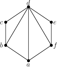


is chordal if it has no induced chordless cycles of size four or more.
However, as Figure 2 shows, the complement of a chordal graph can contain an induced chordless cycle of size four. The complement cannot contain a five cycle though, as the complement of a five cycle is also a five cycle (see Figure 3).
The above example makes it clear why chordal graphs are also weakly chordal.
In this paper, we propose an algorithm that generates a weakly chordal graph from an arbitrary input graph. It is built on top of a subroutine that maintains the weak chordality of a graph , under edge deletion.
3 Arbitrary Graph to Weakly Chordal Graph
3.1 Overview of the Method
We start by generating a random graph on vertices and edges. In a preprocessing step we check if is weakly chordal, using the LB-simpliciality recognition algorithm due to [3]. If is weakly chordal, we stop. Otherwise, we proceed as follows. We first reduce to a chordal graph by introducing additional edges, called fill-edges, using the minimum degree vertex (, for short) heuristic [5]. The heuristic adds edges so that a minimum degree vertex in the current graph is simplicial. Each fill-edge is also entered into a queue, termed a fill-edge queue, . These fill-edges are potential candidates for subsequent deletion from . Since is chordal, it is necessarily weakly chordal. We propose an algorithm for deleting edges from this weakly chordal graph to remove fill-edges, maintaining the weak chordality property. A fill-edge is deleted only if does not create a hole or an anti-hole in the resulting graph and we have developed criteria for detecting this. A fill-edge is removed from the front of the queue, which we then try to delete. If we do not succeed we put it at the back of the queue. We keep doing this until no more fill edges can be removed. Operationally, we implement this by defining a deletion round as one in which the fill-edge at the back of the queue is at the front. We stop when the size of the queue does not change over two successive deletion rounds. Figure 4 is a pictorial illustration of the flow of control.
3.2 Random Arbitrary Graph
To generate a random graph, we invoke an algorithm by Keith M. Briggs, called ‘dense_gnm_random_graph’. This algorithm, based on Knuth’s Algorithm S (Selection sampling technique, see section 3.4.2 of [9]), takes the number of vertices, and the number of edges, , as input and produces a random graph. For a given , we set to a random value lying in the range between and . The output graph may be disconnected, in which case we connect the disjoint components, using additional edges.
3.3 LB-simpliciality test
In [3] Berry et al. proved the following result:
Theorem 3.1
[3] A graph is weakly chordal if and only if every edge is -simplicial.
We apply this recognition algorithm to the random graph generated by the previous step and continue with the next steps only if the recognition algorithm fails. Otherwise, we return .
3.4 Arbitrary Graph to Chordal Graph
The arbitrary graph is embedded into a chordal graph by the addition of edges and the process is known as triangulation or fill-in. Desirable triangulations are those in which a minimal or a minimum number of edges is added. A triangulation of is minimal if is non-chordal for every proper subset of . In a minimum triangulation the number of edges added is the fewest possible. Berry at al. [1] proposed an algorithm, known as LB-Triangulation, for the minimal fill-in problem. LB-Triangulation works on any ordering of the vertices, and produces a fill that is provably exclusion-minimal. In our algorithm, we have used the mdv heuristic [5], as our experiments have shown that this adds fewer fill-edges as compared to LB-Triangulation. We explain this heuristic in the next section.
3.4.1 The Minimum Degree Vertex Heuristic
Let be the graph obtained from , where is set of fill-edges, folllowing these steps. We first assign to and then prune from all vertices of degree 1. From the remaining vertices of we choose a vertex of minimum degree (breaking ties arbitrarily) and turn the neighborhood of into a clique by adding edges. These are fill-edges that we add to the edge set of , as well as to the fill-queue, . Finally, we remove from , the vertex and all the edges incident on it. We repeat this until is empty. The graph is now chordal and is identical with the initial graph , sans degree 1 vertices, and with fill edges added. We illustrate this with an example.

The initial graph is shown in Fig. 5(a) and the graph with all fill-edges added is shown in Fig. 5(b). In the initial graph both and have minimum degree. We break tie in favour of .
Since the induced subgraph on is already a clique no fill-edges are added and is set to . In the reduced
graph , is of minimum degree and the induced graph on is turned into a clique by adding as a fill- edge, which is also added to . Since the reduced graph is a clique, we can pick the vertices
in an arbitrary order to reduce to an empty graph, without introducing any further fill edges into . The formal algorithm is described below:
3.5 Chordal Graph to Weakly Chordal Graph
Since the chordal graph obtained from the previous stage is also weakly chordal, we apply an edge deletion algorithm to that preserves weak chordality. The edges that are candidates for deletion are the ones that have been added by the heuristic. Each candidate edge is temporarily deleted from , and we check if its deletion creates a hole or an anti-hole in . If not, we delete this edge. The process is explained in details in the subsequent sections.
3.5.1 Fill-Edge Queue
As mentioned earlier, each edge added to convert an arbitrary input graph into chordal graph is called a fill-edge. In order to delete as many fill-edges as possible, we maintain a queue of fill-edges, . A fill-edge is removed from the front of this queue, which we then try to delete from . If we do not succeed because a hole or anti-hole is created, we put it at the back of the queue. We keep doing this until no more fill-edges can be removed from .
3.5.2 Detecting Holes
To reiterate, a hole in a graph is an induced chordless cycle on five or more vertices. Since, a graph is weakly chordal if it is (hole, anti-hole)-free [4], it is crucial to detect if any hole is formed by the deletion of an edge. For the class of weakly chordal graphs, since the biggest cycle allowed is of size four, the holes can be formed either by a combination of two ’s or a by a combination of a and a , as illustrated in Fig. 6.
To detect the formation of a hole in , we pick an edge of and temporarily delete it. Now, we check if this deletion creates a hole in . To detect a hole, we perform a breadth-first search in with as the source vertex and find all chordless and paths between and . A hole can be created in two distinct ways: (i) by a disjoint pair of , with six distinct vertices between them such that there exist no chord joining an internal vertex on one to an internal vertex on the other; this we call a hole on two s; (ii) by a disjoint pair of and between and , with five distinct vertices between them, such that there exist no chord joining an internal vertex on the to the internal vertex of the ; this we call a hole on a and a .
3.5.3 Antiholes
An anti-hole in a graph is, by definition, the complement of a hole [4]. An anti-hole configuration in a weakly chordal graphs has the structure shown in Fig. 7. This is an induced graph on six distinct vertices each of which is of degree three.

3.5.4 Detecting Antiholes
To detect an anti-hole configuration, we pick an edge and temporarily delete it from the graph. Next, we check if deleting the edge creates an anti-hole configuration in the graph. To detect this, we do breadth-first search with as the source vertex to find all chordless and paths between and . An anti-hole configuration is formed by a combination of two and one such that the induced graph on the six vertices that define these paths, are uniformly of degree three and there exists a chord from the internal vertex of each to one of the internal vertices in the . For example, in Fig. 7, is a , and are two paths. There exists exactly one chord from to and exactly one from to and, in the induced graph on these six vertices, every vertex has degree three, making it an anti-hole configuration.
3.5.5 Proposed Algorithm
We use an algorithm for deleting edges from a weakly chord graph to remove fill edges, maintaining its weak chordality property. In order to delete as many fill-edges as possible, a fill-edge is removed from the front of the fill-queue, which we then try to delete from . If we do not succeed, we put it at the back of the queue. We keep doing this until no more fill-edges can be removed. Operationally, we implement this by defining a deletion round as one in which the edge at the back of the queue is at the front.
One deletion round comprises of picking an edge from the start of the queue and deleting it from . Now we check if the deletion of creates a hole or an antihole in . If so, we do not delete the edge
and add it back to the fill-queue. Otherwise, we delete the edge from and also remove it from te fill-queue . We stop when the size of does not change over two successive deletion rounds.
For example in Fig. 8, a random arbitrary graph on 6 vertices and 8 edges is obtained. It is converted into a chordal graph by inserting two additional edges. These two additional edges added are put in the fill-edge queue . Maintain a temporary copy of chordal graph in . The deletion algorithm begins by picking first edge in the fill-edge queue and temporarily deletes it from graph to check for hole and antihole configurations. Since deleting does not give rise to any hole or anti-hole configurations, is permanently deleted from starting graph which is now a weakly chordal graph. Now the updated fill-edge queue is . The deletion algorithm now picks the first edge in in the fill edge queue and temporarily deletes it from graph to check for hole and antihole configurations. Since deleting gives rise to a hole configuration on one and one , is not permanently deleted from . Since the queue is now empty, the graph returned by the algorithm is weakly chordal with a small subset of fill-edges added to the original graph .


For another example, consider Figure 9(a), a random arbitrary graph on 6 vertices and 9 edges is obtained. It is converted into a chordal graph (see Figure 9(b)) by adding three additional edges. These three additional edges added are put in the fill-edge queue . Maintain a temporary copy of the chordal graph in . The deletion algorithm begins by picking first edge in the fill edge queue and temporarily deletes it from graph to check for hole and antihole configurations. Since deleting does not give rise to any hole or anti-hole configurations, is permanently deleted from starting graph which is now a weakly chordal graph shown in Figure 9(c). Now the updated fill-edge queue is . The deletion algorithm now picks the first edge in in the fill-edge queue and temporarily deletes it from graph to check for hole and anti-hole configurations. Since deleting does not give rise to any hole or anti-hole configuration, is permanently deleted from starting graph , which is now a weakly chordal graph. Now the updated fill-edge queue is []. The deletion algorithm now picks the first and only edge in the fill-edge queue and temporarily deletes it from graph to check for a hole or an anti-hole configuration. Since deleting gives rise to an anti-hole configuration on two paths , and one , the edge is not permanently deleted from starting graph . Since the queue is now empty, the graph returned by the algorithm is weakly chordal with a small subset of fill-edges added to the original graph as shown in Figure 9(d).
3.6 Complexity
The heuristic can be implemented in time, while the time-complexity of the recognition algorithm based
on LB-simpliciality is in .
To bound the query complexity of deleting an edge from the weakly chordal graph, we note that this is dominated by the task of finding multiple and paths between and and we have to consider these in pairs and run the breadth-first search. An upper bound on the number of pairs of and paths between and is , where and are the degrees of and respectively. For consider such a path from to (see Figure 10): is one of the at most vertices adjacent to and is one of the at most vertices adjacent to , so that we have at most paths from to and thus disjoint pairs of paths from to .
If be the number of edges currently, in the weakly chordal graph, the complexity of running a breadth-first search is . Since is the number of edges in the final weakly chordal graph, an upper bound on the query complexity is .
The deletion of an edge take constant time since we maintain an adjacency matrix data structure to represent .
4 Conclusion
We have proposed a simple method for generating a weakly chordal graph from an arbitrary graph. The proposed algorithm can also be used to generate weakly chordal graphs by deleting edges from input graphs that are known to be weakly chordal, such as complete graphs. Starting with complete graphs also helps in generating dense weakly chordal graphs. An interesting open problem is to establish if the proposed method to generate a weakly chordal graph from an arbitrary graph adds a minimal number of edges.
We have implemented our algorithm in Python. Some sample outputs are shown below in an appendix. In each of the figures,
the purples edges in the chordal graph are edges that are candidates for deletion.
References
- [1] Anne Berry. A wide-range efficient algorithm for minimal triangulation. In Proceedings of the Tenth Annual ACM-SIAM Symposium on Discrete Algorithms, 17-19 January 1999, Baltimore, Maryland, USA., pages 860–861, 1999.
- [2] Anne Berry, Jean Paul Bordat, and Pinar Heggernes. Recognizing weakly triangulated graphs by edge separability. Nord. J. Comput., 7(3):164–177, 2000.
- [3] Anne Berry, Jean Paul Bordat, and Pinar Heggernes. Recognizing weakly triangulated graphs by edge separability. In Algorithm Theory - SWAT 2000, 7th Scandinavian Workshop on Algorithm Theory, Bergen, Norway, July 5-7, 2000, Proceedings, pages 139–149, 2000.
- [4] Carl Feghali and Jirí Fiala. Reconfiguration graph for vertex colourings of weakly chordal graphs. CoRR, abs/1902.08071, 2019.
- [5] Alan George and Joseph W. H. Liu. The evolution of the minimum degree ordering algorithm. SIAM Review, 31(1):1–19, 1989.
- [6] Ryan B. Hayward. Weakly triangulated graphs. J. Comb. Theory, Ser. B, 39(3):200–208, 1985.
- [7] Ryan B. Hayward, Chính T. Hoàng, and Frédéric Maffray. Optimizing weakly triangulated graphs. Graphs and Combinatorics, 5(1):339–349, 1989.
- [8] Ryan B. Hayward, Jeremy P. Spinrad, and R. Sritharan. Improved algorithms for weakly chordal graphs. ACM Trans. Algorithms, 3(2):14, 2007.
- [9] Donald E. Knuth. The Art of Computer Programming, Volume 2/Seminumerical algorithms, Third Edition. Addison-Wesley, 1997.
- [10] Asish Mukhopadhyay, S. V. Rao, Sidharth Pardeshi, and Srinivas Gundlapalli. Linear layouts of weakly triangulated graphs. Discrete Math., Alg. and Appl., 8(3):1–21, 2016.
- [11] Md. Zamilur Rahman, Asish Mukhopadhyay, and Yash P. Aneja. A separator-based method for generating weakly chordal graphs. CoRR, abs/1906.01056, 2019.
- [12] Jeremy P. Spinrad and R. Sritharan. Algorithms for weakly triangulated graphs. Discrete Applied Mathematics, 59(2):181–191, 1995.
- [13] G. Tinhofer. Generating Graphs Uniformly at Random, pages 235–255. Springer Vienna, Vienna, 1990.