Phases of frustrated quantum antiferromagnets on the square and triangular lattices
Abstract
We analyze the zero temperature phase diagrams of the spin quantum antiferromagnet on square and triangular lattices with competing nearest and next-nearest exchange interactions as well as biquadratic couplings. We approach the problem from the large limit. Our primary focus is on determining the extent to which the existence and character of any quantum disordered phases can be inferred from this approach.
I Introduction
A host of interesting quantum disordered phases – including various flavors of quantum spin liquids, valence-bond solids, or quantum nematics – have by now been shown to exist as a matter of principle.Broholm et al. 2020; Wang et al. 2015; Chayes et al. 1989; Xu et al. 2008; Fernandes et al. 2016a; Fernandes et al. 2014; Chubukov et al. 2015 However, the issue of where they exist in the phase diagram of simple models of quantum antiferromagnets with microscopically plausible interactions is still incompletely understood. Various numerical and other approaches have provided strong evidenceJiang et al. 2009; Jiang et al. 2012; Figueirido et al. 1990; Richter et al. 2015; Gong et al. 2014; Capriotti et al. 2001; Iqbal et al. 2016a; Hu et al. 2013; Li et al. 2012; Morita et al. 2015; Wang et al. 2016; Iqbal et al. 2016b; Hu et al. 2015; Kaneko et al. 2014; Zhu and White 2015 that there is a narrow quantum disordered regime in spin and even antiferromagnets near the point at which the classical () model would undergo a transition from an ordered state favored by the nearest-neighbor interaction and that favored when the second-neighbor interaction, is sufficiently large.Chandra et al. 1990; Zhong and Sorella 1993; Chubukov and Jolicoeur 1992
With this physics in mind, we have studied the ground-state phase diagrams of a family of frustrated quantum antiferromagnets on the 2D square and triangular lattices. The classical limit is readily analyzed, and indeed for all the models considered here, this analysis has been carried out previously.Hayden et al. 2010 We have extended these results by computing the leading order (and in some cases higher order) corrections to various quantities in powers of . Much of this analysis has been carried out previously as well.Chandra and Doucot 1988; Fang et al. 2008; Luo et al. 2016; Stanek et al. 2011; Ye and Chubukov 2017; Chernyshev and Zhitomirsky 2009 However, by extending the class of models we have considered, and by taking seriously into account the asymptotic character of the expansion,Castilla and Chakravarty 1991 we have managed to obtain a fuller, and more readily justified picture of the phase diagrams. Since for the classical pure model, the transition point at is highly multi-critical, we have augmented the model studied by including a weak-biquadratic interaction.
Our principle results, as we will discuss, are summarized in the schematic phase diagrams shown in Figs. 1. For the most part at large (where our results are most reliable), instead of an intermediate quantum disordered phase, we find direct first order transitions, for instance between a Neel and stripe phase on the square lattice or the three-sublattice 120o antiferromagnet and the stripe phase on the triangular lattice. However, an exponentially narrow regime of a quantum disordered phase appears on the square lattice between the spin-vortex crystal (SVC) and the conical spin-vortex crystal (CSVC) phases (described in Fig. 2) and between the CSVC and the Neel phase. On the other hand, if we extrapolate our results to smaller , we find evidence for regimes of quantum disordered phases in the same regime of couplings suggested by earlier numerical studies, as also shown in the figure. Not reflected in the figure are a number of subtleties – including the effects of specific topological considerations associated with the quantization of – that can alter the nature of the transitions and of the various quantum disordered phases in the phase diagrams in Fig. 1; we discuss some of these subtleties and other ambiguities in Sec. VI below.


II The model
We considered interacting spin operators on a regular lattice, with nearest and next-nearest-neighbor quadratic interactions as well as nearest-neighbor biquadratic interactions
| (1) | |||||
where satisfy canonical commutation relations for spin operators, with . Since we will always assume that the nearest-neighbor exchange coupling, , we can chose units of energy such that as in the above. We will consider explicitly the cases of a square and a triangular lattice. Here and denote nearest and next-nearest neighbors respectively and signifies sites forming minimal squares on the lattice. We have normalized the interactions so that the ground-state energy density has a well defined limit, when the spins can be treated as classical Heisenberg rotors.
For large the effects of and are very similar. For the most part, we will report explicit results for , as this is slightly more convenient for the large analysis. However, there is a significant difference for , where can be incorporated exactly into a renormalized value of , while remains an independent coupling constant. Thus, when extrapolating our results to , one should loosely interpret as a proxy for .
III Classical phase diagrams
III.1 The square lattice
The zero temperature classical phase diagram in the plane for square lattice was discussed in Ref. Hayden et al. 2010, and is summarized in Figs.2.
When , there is a first order phase transition between the collinear Neel and the collinear stripe phases at . By contrast, for and of small magnitude, there are three phases as a function of increasing : a Neel phase, a non-coplanar conical spin-vortex crystal (CSVC) phase, and a coplanar (non-collinear) spin-vortex crystal (SVC) phase. The SVC state, illustrated in Fig.2, consists of alternating spin-vortices on neighboring plaquettes, oriented with respect to a spontaneously chosen “X-Y” plane in spin-space. The CSVC can be thought as a linear combination of the Neel and SVC states, with spin-components in the preferred X-Y plane oriented as in a SVC state, while the z components exhibit Neel-type order. It can thus be viewed as a state with coexisting Neel and SVC order, and correspondingly the two phase transitions at and are continuous. As we will focus only on reasonably small , we will neglect the spiral phase that arises when is large and negative.
Note that is a non-generic line along which the classical ground states at are highly degenerate. Here the analysis is subtle, involving effects of “order from disorder.”

III.2 The triangular lattice
The zero temperature classical phase diagram in the plane for the triangular lattice is summarized in Fig.3. For there is a first order phase transition from a three-sublattice phase for to a two-subblattice stripe phase for larger . For , the system undergoes a first order phase transition from the phase to a four-sublattice non-coplanar spin-tetrahedron crystal (STC) phase at a critical value of .

The and stripe phases are shown schematically in Fig.3. The STC has a 4 sublattice structure, as also shown, such that the four spins (up to a global rotation) point in the direction of the four vertices of a tetrahedron. It is easily checked that this configuration minimizes the repulsive biquadratic interaction in the 4-sublattice decomposition. We will restrict attention to relatively small biquadratic interactions , and small ; other interesting phases could appear for stronger interactions.
IV First order () quantum corrections
A systematic formalism for computing quantum fluctuations about the classical ground-state can be accomplished using a Holstein-Primikoff (HP) transformation to map the problem into a problem of weakly interacting bosons. The first order corrections in powers of are obtained by keeping terms to quadratic order in the bosonic fields - i.e. treating the quantum fluctuations as non-interacting spin-waves. Higher order corrections in powers of can be computed, in principle, by treating the interactions between bosons perturbatively. This formalism, and the details of specific calculations are reviewed in the appendix. In this section, we report on the quantum corrections to various quantities computed to first order in .
The ground-state energy per lattice site of a system in a given state labeled by (for example, Neel) is
| (2) | |||||
where is the classical ground-state energy, is the number of sites, are the normal mode frequencies, (which specifies the Bloch wave-number and possibly other quantum numbers where necessary) labels the individual normal modes, is a constant term proportional to K from terms in various of non-collinear states, and indicates higher order terms in powers of . In particular, the non-interacting part of the HP Hamiltonian can be expressed in terms of bosonic creation operators, , as where the coefficients and depend on the nature of the classical ordered state that serves as the starting point, and
| (3) |
Manifestly, this calculation only makes sense so long as is real for all , i.e. that . This is equivalent to the condition that the classical configuration be at least metastable. The specifics of the calculations of and for each of the relevant states are discussed in the Appendix.
Similarly, we will compute the anomalous expectation values of the various order parameters that characterize aspects of the broken symmetries of the various phases:
| (4) |
where we will always normalize so that the classical expectation value of its magnitude is 1, and is a function of and . In particular, the sublattice magnetization of the various phases is defined as
| (5) |
where is a unit vector in the direction (in spin-space) of the corresponding classical orientation of spin at site . Again, the explicit calculations pertinent to computing are summarized in the Appendix.
Needless to say, this expansion is strictly justified only when the corrections to the classical results are small. Where there is a first order transition, the order parameter is generally non-zero even proximate to the transition. We can determine the location of such phase boundaries by comparing the energy per site, , of the two relevant phases. Thus, the first order corrections to the position of such a phase boundary (e.g. the critical value of ) can be directly computed from the first order expression for the ground-state energies.
We will also makes estimates of the points at which quantum fluctuations become sufficiently large that they cause a classical order parameter to vanish. Here we are always extrapolating our results beyond the range in which the spin-wave expansion is controlled. Moreover, since the expansion is known to be an asymptotic series, there is no reason to think that this estimate would be improved by keeping higher order terms in the expansion (at least without employing additional information to allow a resumation of the series). None-the-less, it is instructive to extrapolate the results to the point at which the leading order expression for each order parameter would vanish; in this way, we interpret as an estimate of the critical value of at which each of these order parameters would vanish (baring any other preemptive phase transition that destroys the order at larger ).
IV.0.1 Square lattice with
The two pertinent phases for are the Neel and the stripe phase. Both are states with non-zero sublattice magnetization, , with Neel and str (for stripe order). The stripe phase also breaks the lattice 4-fold rotational symmetry in a manner that is characterized by the nematic order parameter,
| (6) |
The factor of is included so that in the classical stripe-ordered state, , so that is defined as in Eq. 4.
The first order quantum corrections to all these orders were computed previously.Fang et al. 2008 We have added to these results expressions for the first order shifts in the ground-state energies, .
Since the classical transition between the Neel and stripe phases is first order, the correction to the location of the phase boundary can be computed directly by identifying the point at
| (7) |
This is indicated by the heavy purple line in Fig. 4. Note that quantum fluctuations stabilize the Neel state relative the stripe-ordered state. The line terminates at a value of at which the classical Neel state ceases to be metastable; to determine the nature of the phase boundary at larger values of (smaller ) we will need to rely on indirect arguments, as we will discuss below. The remaining lines in Fig. 4 show the calculated values of vs. . As is clear from the figure, for all three orders, the values of vanish as a critical value that depends on the nature of the order involved. This would seem to indicate that at this point the corresponding classical phase is unstable to quantum disordering even for arbitrary large so long as is not infinite. However, for large (where our calculations are controlled) these putative quantum disordering transitions are pre-empted by the first order transition already discussed. In addition, it is worth noting that is negative for intermediate ( to at ), which means first order quantum correction could enhance the nematic order. We will return to these results in Sec. V below, where we will present arguments to determine the nature of the phases in various regions labeled by letters in Fig. 4.

The K-dependence of the various quantities at fixed are shown in Fig.5. The thin lines indicate and the heavy purple line marks the point at which one would conclude from the expressions computed to first order in . The solid lines show results for while the dashed lines are for . The dashed-dotted line is where the classical Neel state starts/ends to be metastable. It is not the true boundary between nematic and stripe regime, but will later be useful in Sec. V to estimate the true boundary.

IV.0.2 Square lattice with
The relevant phases for are the Neel, spin-vortex crystal (SVC) and conical spin-vortex crystal (CSVC). All are states with non-zero sublattice magnetization, , with Neel, SVC, and CSVC. In addition, we define composite order parameters that capture specific aspects of the broken symmetry of various phases. As with the more familiar case of nematic order arising as “vestigial orderNie et al. 2014” upon partial melting of a stripe-ordered state, it is possible to conceiveFernandes et al. 2016b of phases with vestigial broken symmetries that arise by partial melting of, respectively, a SVC or a CSVC phase such that the primary order parameter vanishes but the composite order parameters remain finite. Specifically, we define
| (8) |
which we will refer to as the spin-nematic vortex crystal (SNVC) and chiral (chir) order parameters. Here . These order parameters are, respectively, an axial vector and a pseudo-scalar in spin-space, both normalized so that their magnitude is 1 in a corresponding classically ordered state. A phase with but thus breaks spin-rotational order in the same sense as a spin-nematic, as well as breaking translational symmetry. (From a broken symmetry perspective, it is equivalent to a triplet d-density wave.Hsu et al. 2011.) A phase with but preserves spin-rotational and translational symmetries, but has net spin chirality.
The dashed lines in Fig. 2 represent continuous transitions at between states that break distinct symmetries; since the CSVC interpolates between the Neel and the SVC phase, such transitions are in principle consistent with Landau theory. However, what is not generic is that upon approaching the transition from either side, both phases cease to be metastable (i.e. an appropriate spin-wave velocity vanishes) along the phase boundaries. Consequently, we expect that for finite , an intermediate region with neither form of magnetic order occurs.
Indeed, as shown in Fig. 6, the curves of vs for the various phases diverge from each other slowly as is tuned away from its critical value, as
| (9) |
where in this expression near the convergence of the solid blue and solid orange lines (for and ) and near the convergence of the solid orange and solid yellow lines (for and ). Note that for each value of , this expression only applies as one approaches the critical value from the appropriate direction and that in all cases with values that we compute explicitly in the appendix. These results strongly suggest that, even for large , quantum disordered phases arise near between the Neel and CSVC phases, shown as the green shaded regions in Fig. 6, and near between the CSVC and SVC phases, which is too narrow to show up as a shaded region but is also indicated in the figure. Note that the purple line marking the contour at which the extrapolated chiral order vanishes lies inside a quantum disordered region suggesting that there are (at least) two distinct phases here - one with vestigial chiral order and one that is more fully quantum disordered. We will return to these results in Sec. V below for smaller , where we will present arguments to determine the nature of the phases in the various regions labelled by letters in Fig. 6.

The K-dependence of the various quantities at fixed spin are shown in Fig.7. Solid lines indicate from the expressions computed to first order in . Classical () phase boundaries are added as dashed lines.


IV.0.3 Triangular lattice with
The two pertinent phases for are the and the stripe phase. Both are states with non-zero sublattice magnetization, , with and str (for stripe order). The stripe phase also breaks the lattice 6-fold rotational symmetry in a manner that is characterized by the (three-state) nematic order parameter,
| (10) | |||
Here, with , 2, or 3 are the unit vectors on the triangular lattice, and in the classical stripe-ordered state in which the spins on site and have the opposite spin orientation as the spins on sites and , while for the two other classical stripe ordered states. Like the spin vortex crystal phase in the square lattice, phase also breaks the spin rotational symmetry. The vestigial phase can be characterized by the spin-nematic vortex crystal order:
| (11) |
The sum is among all set of spins in clockwise order (vorticity), within type A triangles (). The sum for spins also in clockwise order within type B triangles () can be shown to be exactly opposite. A phase with but thus breaks spin-rotational order, but, in contrast with the SNVC phase on the square lattice, it does not break translational symmetry.
Since the classical transition between the and stripe phase is first order, the correction to the location of the phase boundary can be computed directly by identifying the point at
| (12) |
This is indicated by the heavy purple line in Fig.8. Note that quantum fluctuations stabilize the stripe state relative the state. The line terminates at a value of at which the classical stripe state ceases to be metastable; The remaining lines in Fig. 8 show the calculated values of vs. . As is clear from the figure, for all four orders, approaches non-zero values as a critical value that depends on the nature of the order involved.

The K-dependence of the various quantities at fixed are shown in Fig.9. Representative of the large spin case, the line in the plane along which for is marked by the heavy dashed purple line; no solution of this equation exists in the small spin case, . Conversely, the lines on which in the small spin case, , are marked by the thin solid lines; no such lines exist at large spin .

IV.0.4 Triangular lattice with
The two pertinent phases for are the and the spin-tetrahedron crystal phase. Both are states with non-zero sublattice magnetization, , with and STC (for spin-tetrahedron crystal order).
Since the classical transition between the and STC phase is first order, the correction to the location of the phase boundary can be computed directly by identifying the point at which . In the classical limit, this occurs at the limit of metastability of the phase. Moreover, in the entire regime in which both states are classically metastable, the phase always has a lower energy even when first order quantum corrections are included. Thus, this first order phase boundary does not vary with to first order in ; the first order boundary between phase and STC phases occurs at in Fig.10.

The K-dependence of the various quantities at fixed spin are shown in Fig.11. Thin solid lines indicate from the expressions computed to first order in .
V Extrapolation to smaller
While there are surely dangers involved, it is worth-while extrapolating the results that are controlled at large to form at least a conjectural completion of the phase diagrams, as shown in Fig. 1. This also allows us to make contact with a host of numerical studies that have been performed on the same models for the cases of and . In this section, we outline the logic that leads to this figure. In all cases, when we refer to “the ground state energy” or “the magnitude of the order parameter” we are implicitly referred to quantities that are computed to leading order in . For example, when we refer to a region of the phase diagram in which the Neel order parameter vanishes, we mean a region where , i.e. where the extrapolated magnitude of the order parameter would be negative.
V.1 Square lattice with
Our analysis of the square lattice with is based on identifying the nature of the ground-state in the various regions shown in Fig. 4 which are labelled by different letters. Everywhere to the left of the solid purple line (i.e. regions A, C, and D) the energy of the Neel state is lower than the stripe phase, implying that the stripe phase is excluded in all these regions. In region A (i.e. below the blue line) the magnitude of is positive, so we identify this as being approximately the region in which Neel order survives quantum fluctuations. Conversely, in regions C and D, vanishes, which we interpret as meaning that no magnetic order survives in either region. Indeed, in region D all the orders we have considered are precluded, so we identify it as a fully quantum disordered regime. On the other hand, in region C quantum fluctuations of the nematic order do not vanish cause it to vanish, so we conjecture that this corresponds to a nematic phase. Similarly all of region (B) is likely stripe ordered, since the stripe state is energetically preferred, and its order parameter including first order quantum corrections is non-zero.
The nature of phase transitions can now be considered. The transition indicated by the heavy purple line in Fig. 4 between the Neel and stripe phases is first order, and is unambiguously calculable when is large. Since we have identified the phase transitions between different regions separated by thin solid lines as the points at which quantum fluctuations become large enough that one or another order parameter vanishes, we have implicitly assumed that these transitions are all continuous. For the cases of the Neel to disordered (A to D) and the nematic to disordered (C to D), these correspond to reasonable Landau-allowed order to disorder transitions. However, the implied Neel to nematic transition (A to C) is not Landau allowed, and indeed to the extent that the first order in expressions can be trusted, the nematic order would have a finite jump across this transition. While, as discussed in Sec. VI, under special conditions, a “beyond Landau” continuous deconfined quantum critical transitionSenthil et al. 2004 between a Neel and a quantum nematic paramagnet is possibleWang et al. 2015, far more likely is that the transition between these two phases is first order and probably not quite at the same point as the solid blue line. The nature of the phase transition between the nematic and stripe phases is also unclear. This is Landau-allowed to be continuous although at least where it occurs along the heavy purple line it is probably first order. If we were to extend the range of parameters shown in Fig. 4 we would find that the orange line and the green line cross at ; we interpret this crossing as a bicritical point marking the end of the first order stripe to nematic phase boundary, beyond which a direct stripe to quantum disordered transition is expected.
The K-dependence of phase diagram can be obtained from the same sort of analysis. Contours of and lines of in Fig. 5 are now used to estimate the phase boundaries. Phases (A) Neel, (B) stripe, (C) nematic and (D) quantum disordered are explicitly labelled for . For small , the width of the ”nematic-like” phase (C), and of the quantum disordered phase (D) – indicated by the black arrows in the main panel of Fig.5), become exponentially small as increases, and so are invisible for .
Together, these considerations lead to the schematic phase diagram shown in Fig.1(a).
V.2 Square lattice with
For the square lattice with , the analysis that leads from Figs. 6 and 7 to the schematic phase diagram in Fig.1(b) is relatively straightforward. Specifically, as can be seen in Fig. 6, the basic topology of the phase diagram is already established when is large, and hence can be interpreted without need of extrapolating to smaller . Thus regions A, B, C, D, and E correspond to Neel, SVC, CSVC, chiral and quantum disordered phases, respectively.
The nature of phase transitions can now be considered. Again, since we have identified the phase transitions as the points at which quantum fluctuations become large enough that one or another order parameter vanishes, we have implicitly assumed that these transitions are all continuous. All the phase transitions here are Landau-allowed to be continuous. The K-dependence phase diagram can be obtained from the same sort of analysis. In common with the case, the width of the quantum disordered phase (E), and of the chiral phase(D) – indicated by black arrow in Fig.7 – decreases exponentially as S increases. However, one noticeable difference is that the quantum disordered regime is present even at large in the phase diagram with . Note that both CSVC and chiral phases requires sufficiently large to develop non-zero order parameters. Therefore, at small , the width of quantum disordered phase increase as increases. This can be traced back to the fact that “order by disorder” phenomenaChandra et al. 1990 effectively addLarson and Henley 2008 a positive contribution to which tends to stabilize the two collinear states (Neel and stripe).
These consideration lead to the schematic phase diagram shown in Fig.1(b), in which phase boundary between chiral and CSVC phase have been extended and connected to larger for artistic reasons.
V.3 Triangular lattice with
The schematic phase diagram for the triangular lattice with shown in in Fig. 1(c) is obtained by identifying the most likely phase corresponding to the different labeled retions in Figs. 8 and 9 which are labelled by different letters. Everywhere to the left of the solid purple line in Fig. 8 (i.e. regions A and D) the energy (where it can be computed) of the state is lower than that of the stripe phase, implying that the stripe phase is excluded. In region A (i.e. below the blue line) the magnitude of is positive, so we identify this as the region in which order survives quantum fluctuations. However, in regions D, vanishes, which we interpret as meaning that no magnetic order survives in this region. Indeed, in region D all the orders we have considered are precluded, so we identify it as a fully quantum disordered regime. Similarly all of region B is likely stripe ordered, since the stripe state is energetically preferred, and its order parameter including first order quantum corrections is non-zero. In region C, the nematic order does not vanish, while stripe order vanishes and phase is energetically excluded; so we conjecture that this corresponds to a nematic phase.
The nature of phase transitions can now be considered. The analysis closely parallels that of the square lattice with . The transition indicated by the heavy purple line in Fig. 8 between the and stripe phases is first order, and is unambiguously calculable when is large. Since we have identified the phase transitions between different regions separated by thin solid lines as the points at which quantum fluctuations become large enough that one or another order parameter vanishes, we have implicitly assumed that these transitions are all continuous. For the cases of the to disordered (A to D) and the nematic to disordered (C to D), these correspond to reasonable Landau-allowed order to disorder transitions. However, the implied to nematic transition (A to C) is not Landau allowed, and indeed to the extent that the first order in expressions can be trusted, the nematic order would have a finite jump across this transition. It is thus likely that the transition between these two phases is first order and probably not quite at the same point as the solid blue line. The nature of the phase transition between nematic and stripe phase is also unclear. This is Landau-allowed to be continuous. Different from square lattice, we are unable to extend the range of parameters shown in Fig. 8 to larger , since there are other relevant phase. Thus, we are unable to confirm the existence of a bicritical point marking the end of the first order stripe to nematic phase boundary, beyond which a direct stripe to quantum disordered transition is expected.
The K-dependence of phase diagram can be obtained from the same sort of analysis. Contours of for (dashed lines) and line of for (solid line) in Fig. 9 are now used to estimate the phase boundaries. Phases (A) , (B) stripe, (C)nematic-like and (D)quantum disordered are explicitly labelled for . Contrary to the results of square lattice, since quantum correction to order parameter does not have the logarithmic divergence as approaches the critical value , the width of the nematic and quantum disordered phase does not decay exponentially as S increases. It has been shown in Fig.8 that these two phases do not appear at large spin.
V.4 Triangular lattice with
Finally, we use the results in Figs. 10 and Fig.11 to construct the qualitative phase diagram for the triangular lattice with shown in Fig. 1(d). It should be noted that the solid line in Fig. 10 indicating the value of for STC is not shown since corresponding to an unphysical value of . For region A under the blue line the order parameter is apparently non-zero. We thus identify region A with the phase. Region B is identified with the STC phase, since only the STC state is metastable, and its order parameter is estimated to be non-zero. Region C is not in the nor the STC phase, since the order parameter vanishes, and the STC state has a higher energy than the state. It may be in a quantum disordered phase, or another symmetry breaking vestigial phases that we have not considered. The K-dependence phase diagram at fixed is summarized in Fig.11. As is the case with the square lattice, quantum fluctuations tend to stabilize the positive phases relative to those with negative as a form of order from disorder.
The phase boundaries are now given by two lines. One is the blue line for in Fig.10, that separates the phase and the quantum disordered phase. Another one is at , where classical state ceases to be metastable, that separate STC phase with other two phases. The phase transition between the phase and the quantum disordered phase should be continuous, since the order parameter vanishes continuously upon approaching the phase boundary. The phase transitions between STC phase and the other two phases ( and quantum disordered phase) should be first-order, since the STC order parameter is non-zero upon approaching the phase boundaries.
V.5 Comments on the validity of the extrapolation
Based on the above extrapolation of the first order in expansion to smaller , we obtained the schematic phase diagrams in Fig.1. As stated in the beginning of this section, the extrapolation is dangerous and its validity cannot be guaranteed. However, in this subsection, we would like to comment on the validity of this extrapolation, by comparing the results fn the first order expansion with the second order the expansion. Since the expansion is an asymptotic series,Castilla and Chakravarty 1991 where the first and second order results differ substantially, it is far from clear which is closer to the correct answer. Therefore, this comparison only functions as a “comment” rather than any systematic proof of the validity of the above extrapolations.
For illustration purpose, we only focus on the stability of the stripe phase on the square lattice with . This has been calculated in Majumdar 2010, for the case without a biquadratic interaction. In general, the biquadratic interaction can be approximated by the following quadratic interaction.
| (13) |
and if the classical configuration is collinear, can then be replaced by its classical expectation value. For the stripe phase, the above mean-field approximation leads an anisotropic term, which has already been included in the previous study Majumdar 2010.
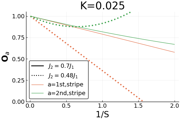
As a function of , the stripe order parameter under zeroth order (classical result, blue line), first order (orange line) and second order (green line), as well as nematic order parameter under first order (purple line) expansion are plotted in Fig.12. Solid lines are for , and dashed lines are for . As grows, the second order results starts deviating from the first order quantum correction. The first order result on should not be trusted if the deviation is big. Therefore, as , the order parameter from first order quantum correction becomes trustable only at large spin.
In our previous extrapolations, we use to estimate the true phase boundary . This estimation in general works better at larger spin and further away from the critical point.
VI Beyond spin-wave analysis
There are a large number of additional subtleties that we have overlooked in the present analysis. We have treated as a continuous parameter that tunes the extent of the quantum oscillations – this is very similar in spirit to the classic approach of Ref. Chakravarty et al. 1989. However, is in fact a discrete variable, and there can be differences in the physics depending on whether it is integer or half-integer,Haldane 1988; Read and Sachdev 1989; Senthil and Fisher 2006 and even whether it is an even integer or an odd integerAffleck et al. 2004; Wang et al. 2015. This can effect the nature of the allowed phases and opens up the possibility of exotic, beyond Landau deconfined quantum phase transitions.Senthil et al. 2004 For instance, generalizations of the famous Lieb-Schulz-Mattis theoremLieb et al. 1961; Yamanaka et al. 1997; Hastings 2004, imply that the disordered phase for a half-integer spin must either have a broken symmetry (e.g. exhibit valence-bond-crystalline order) or be one or another of quantum spin liquid with topological order.
Since most of the numerical studies to date have been carried out for , or, to a lesser extent, for , these additional subtleties are likely to be significant. However, we can still distinguish magnetically ordered phases from quantum disordered phases. Moreover, within the regime of quantum disordered phases, we may be able to distinguish those that exhibit broken symmetries as a form of vestigial order, if the order is accompanied by reasonably long but still finite range correlations that reflect the structure of a nearby magnetically order, vs. broken symmetries (such as the before mentioned topological order) that are more readily identified with topological terms in the effective field theorySenthil and Fisher 2006, rather than with any proximate magnetically ordered state.
Intense effort and enormous creativity has been marshaled for the numerical search for intermediate non-magnetic quantum-disordered states in the models (wiht ). For on the square Richter et al. 2015; Gong et al. 2014; Capriotti et al. 2001; Iqbal et al. 2016a; Hu et al. 2013; Li et al. 2012; Morita et al. 2015; Wang et al. 2016; Jiang et al. 2012; Figueirido et al. 1990 and triangular lattice Iqbal et al. 2016b; Hu et al. 2015; Kaneko et al. 2014; Zhu and White 2015, various of numerical works have confirmed the existence of an intermediate quantum disordered state(s). However, the nature of the intermediate state(s) is still under debate. For on a square lattice, there is contradictory evidence concerning the existence of intermediate phases; Haghshenas et al. 2018; Bishop et al. 2008; Jiang et al. 2009 notably, in the studyJiang et al. 2009 that is most strongly indicative of the occurrence of such a phase, it is found to occur in an exceedingly narrow range of and to have a clear nematic character. We are unaware of any studies of the model on the triangular lattice. Since finite S effectively adds a positive K, one should compare the above numerical studies with the phase diagrams in our work with . At least in terms of the general topology of the phase diagram, the results of the existing numerical studies appear to be consistent with those shown in Figs. 1 a and c. An interesting future direction for numerical studies suggested by the present study is to investigate the model with negative (or for ) where the quantum disordered phases are found to persist to large and to have a broader region of stability.
VII conclusion
We analyzed Heisenberg model on square and triangular lattice with nearest neighbor and next-nearest neighbor quadratic interactions, as well as nearest-neighbor biquadratic interaction at zero temperature. We analyzed the effect of the biquadratic interaction, and obtained phase diagram under first order quantum correction using linear spin wave theory. We compared our results on repulsive biquadratic interaction with the previously works on attractive interaction.
We found that the classical first order transition under attractive biquadratic interaction is preserved at large spin. The classical continuous phase transitions under repulsive biquadratic interaction is however replaced by quantum disordered regions. Those quantum disorder regions exist for arbitrary and reasonably small K. We computed first order quantum corrections to short-range order parameters for non-collinear and non-coplanar states under repulsive biquadratic interaction, and observed the short-range ordered conical vortex lattice state on the square lattice. Our work on nearest neighbor repulsive biquadratic interaction points towards new regimes to search for interesting behaviors in future numerical work.
Aknowdegements: We would like to acknowledge helpful discussions and suggestions from H-C. Jiang, P. Coleman, P. Chandra, Y. Jiang, F. Wang, and R. Tomalle. SAK was supported, in part, by NSF grant # DMR-1608055 at Stanford.
References
- Broholm et al. (2020) C. Broholm, R. Cava, S. Kivelson, D. Nocera, M. Norman, and T. Senthil, Science 367 (2020).
- Wang et al. (2015) F. Wang, S. A. Kivelson, and D.-H. Lee, Nature Physics 11, 959 (2015).
- Chayes et al. (1989) J. Chayes, L. Chayes, and S. Kivelson, Communications in mathematical physics 123, 53 (1989).
- Xu et al. (2008) C. Xu, M. Müller, and S. Sachdev, Physical Review B 78, 020501 (2008).
- Fernandes et al. (2016a) R. Fernandes, S. Kivelson, and E. Berg, Physical Review B 93, 014511 (2016a).
- Fernandes et al. (2014) R. M. Fernandes, A. V. Chubukov, and J. Schmalian, Nature physics 10, 97 (2014).
- Chubukov et al. (2015) A. V. Chubukov, R. M. Fernandes, and J. Schmalian, Physical Review B 91, 201105 (2015).
- Jiang et al. (2009) H. Jiang, F. Krüger, J. Moore, D. Sheng, J. Zaanen, and Z. Weng, Physical Review B 79, 174409 (2009).
- Jiang et al. (2012) H.-C. Jiang, H. Yao, and L. Balents, Physical Review B 86, 024424 (2012).
- Figueirido et al. (1990) F. Figueirido, A. Karlhede, S. Kivelson, S. Sondhi, M. Rocek, and D. Rokhsar, Physical Review B 41, 4619 (1990).
- Chandra et al. (1990) P. Chandra, P. Coleman, and A. Larkin, Physical review letters 64, 88 (1990).
- Zhong and Sorella (1993) Q. Zhong and S. Sorella, EPL (Europhysics Letters) 21, 629 (1993).
- Chubukov and Jolicoeur (1992) A. V. Chubukov and T. Jolicoeur, Physical review B 46, 11137 (1992).
- Hayden et al. (2010) L. X. Hayden, T. A. Kaplan, and S. D. Mahanti, Phys. Rev. Lett. 105, 047203 (2010), URL https://link.aps.org/doi/10.1103/PhysRevLett.105.047203.
- Chandra and Doucot (1988) P. Chandra and B. Doucot, Phys. Rev. B 38, 9335 (1988), URL https://link.aps.org/doi/10.1103/PhysRevB.38.9335.
- Fang et al. (2008) C. Fang, H. Yao, W.-F. Tsai, J. Hu, and S. A. Kivelson, Phys. Rev. B 77, 224509 (2008), URL https://link.aps.org/doi/10.1103/PhysRevB.77.224509.
- Luo et al. (2016) C. Luo, T. Datta, and D.-X. Yao, Physical Review B 93, 235148 (2016).
- Stanek et al. (2011) D. Stanek, O. P. Sushkov, and G. S. Uhrig, Physical Review B 84, 064505 (2011).
- Ye and Chubukov (2017) M. Ye and A. V. Chubukov, Physical Review B 95, 014425 (2017).
- Chernyshev and Zhitomirsky (2009) A. Chernyshev and M. Zhitomirsky, Physical Review B 79, 144416 (2009).
- Castilla and Chakravarty (1991) G. E. Castilla and S. Chakravarty, Physical Review B 43, 13687 (1991).
- Nie et al. (2014) L. Nie, G. Tarjus, and S. A. Kivelson, Proceedings of the National Academy of Sciences 111, 7980 (2014).
- Fernandes et al. (2016b) R. Fernandes, S. Kivelson, and E. Berg, Physical Review B 93, 014511 (2016b).
- Hsu et al. (2011) C.-H. Hsu, S. Raghu, and S. Chakravarty, Physical Review B 84, 155111 (2011).
- Senthil et al. (2004) T. Senthil, A. Vishwanath, L. Balents, S. Sachdev, and M. P. Fisher, Science 303, 1490 (2004).
- Larson and Henley (2008) B. E. Larson and C. L. Henley, Effective hamiltonians for state selection in heisenberg antiferromagnets (2008), eprint 0811.0955.
- Majumdar (2010) K. Majumdar, Phys. Rev. B 82, 144407 (2010), URL https://link.aps.org/doi/10.1103/PhysRevB.82.144407.
- Chakravarty et al. (1989) S. Chakravarty, B. I. Halperin, and D. R. Nelson, Physical Review B 39, 2344 (1989).
- Haldane (1988) F. D. M. Haldane, Phys. Rev. Lett. 61, 1029 (1988), URL https://link.aps.org/doi/10.1103/PhysRevLett.61.1029.
- Read and Sachdev (1989) N. Read and S. Sachdev, Physical review letters 62, 1694 (1989).
- Senthil and Fisher (2006) T. Senthil and M. P. Fisher, Physical Review B 74, 064405 (2006).
- Affleck et al. (2004) I. Affleck, T. Kennedy, E. H. Lieb, and H. Tasaki, in Condensed Matter Physics and Exactly Soluble Models (Springer, 2004), pp. 249–252.
- Lieb et al. (1961) E. Lieb, T. Schultz, and D. Mattis, Annals of Physics 16, 407 (1961).
- Yamanaka et al. (1997) M. Yamanaka, M. Oshikawa, and I. Affleck, in APS March Meeting Abstracts (1997).
- Hastings (2004) M. B. Hastings, Physical review b 69, 104431 (2004).
- Richter et al. (2015) J. Richter, R. Zinke, and D. J. Farnell, The European Physical Journal B 88, 2 (2015).
- Gong et al. (2014) S.-S. Gong, W. Zhu, D. Sheng, O. I. Motrunich, and M. P. Fisher, Physical review letters 113, 027201 (2014).
- Capriotti et al. (2001) L. Capriotti, F. Becca, A. Parola, and S. Sorella, Physical review letters 87, 097201 (2001).
- Iqbal et al. (2016a) Y. Iqbal, P. Ghosh, R. Narayanan, B. Kumar, J. Reuther, and R. Thomale, Physical Review B 94, 224403 (2016a).
- Hu et al. (2013) W.-J. Hu, F. Becca, A. Parola, and S. Sorella, Physical Review B 88, 060402 (2013).
- Li et al. (2012) T. Li, F. Becca, W. Hu, and S. Sorella, Physical Review B 86, 075111 (2012).
- Morita et al. (2015) S. Morita, R. Kaneko, and M. Imada, Journal of the Physical Society of Japan 84, 024720 (2015).
- Wang et al. (2016) L. Wang, Z.-C. Gu, F. Verstraete, and X.-G. Wen, Physical Review B 94, 075143 (2016).
- Iqbal et al. (2016b) Y. Iqbal, W.-J. Hu, R. Thomale, D. Poilblanc, and F. Becca, Physical Review B 93, 144411 (2016b).
- Hu et al. (2015) W.-J. Hu, S.-S. Gong, W. Zhu, and D. Sheng, Physical Review B 92, 140403 (2015).
- Kaneko et al. (2014) R. Kaneko, S. Morita, and M. Imada, Journal of the Physical Society of Japan 83, 093707 (2014).
- Zhu and White (2015) Z. Zhu and S. R. White, Physical Review B 92, 041105 (2015).
- Haghshenas et al. (2018) R. Haghshenas, W.-W. Lan, S.-S. Gong, and D. Sheng, Physical Review B 97, 184436 (2018).
- Bishop et al. (2008) R. F. Bishop, P. H. Y. Li, R. Darradi, and J. Richter, EPL (Europhysics Letters) 83, 47004 (2008), URL https://doi.org/10.1209%2F0295-5075%2F83%2F47004.
Appendix A Holstein-Primakoff transformation for coplanar(including collinear) configuration
In this section, we would like to review a systematic way to perform Holstein-Primakoff transformation, if the classical configuration is coplanar. This will eventually lead to a translational invariant Hamiltonian, in terms of creation and annihilation operators, for Neel, stripe and SVC state. Without loss of generality, let us suppose spins in the classical configuration is in xz plane .
If , the standard Holstein-Primakoff transformation is
| (14) |
Here, we have already taken the leading order contribution in HP transformation. Generally, for arbitrary , we can choose
| (15) |
Now we would like to explicitly write down , up to quadratic terms in terms of bosonic operators. The constant term is if and are different spin, and if . This will be important when calculating ground state energy. The linear terms in are
| (16) |
, which is useful in the biquadratic interaction , which contains the square of the above linear terms. The quadratic terms in is
| (17) |
is the angle difference between and in the classical configuration.
For the coplanar Neel, stripe and SVC phase, and for nearest neighbored and next-nearest neighbored spins is invariant under translation. Therefore, a translational invariant Hamiltonian in terms of creation and annihilation operators is expected.
In the next subsections, we will explicit derive the resulted Hamiltonian for Neel and stripe phase. We will include the result for SVC phase.
A.1 square lattice-Neel & stripe phase
In this section, we consider the general ordering vector , which describes the Neel-stripe transition. For the nearest neighbored terms, angle difference is along x-direction and along y-direction. Plugging in the Holstein-Primakoff transformation in Eq.17, we get
| (18) |
Noted that the summation along x and y are separately written down. For second nearest neighbored terms, the angle difference is . After Holstein-Primakoff transformation, we have
| (19) |
For the biquadratic terms, we first perform mean-field approximation, and then Holstein-Primakoff transformation:
| (20) |
N is the total number of sites.
Now we can perform Fourier transformation
| (21) |
We have
| (22) |
By taking , we can reproduce the result for stripe and Neel phase, as obtained in (Fang et al. 2008).
A.2 square lattice-SVC phase
In the classical configuration for the SVC state, the angle between nearest neighbors is , and the angle difference between next-nearest neighbors is . The Hamiltonian in terms of bosonic operators is
| (23) |
A.3 triangular lattice- phase stripe phase
In this section, we will apply Holstein-Primakoff transformation to the coplanar phase and stripe phase. We will explicitly derive the phase, while provide the result for the stripe phase.
For phase, the angle difference is for all nearest neighbors. Plugging in the Holstein-Primakoff transformation, we get
| (24) |
For the next-nearest neighbored terms, angle difference is , that leads to
| (25) |
Biquadratic terms can be treated by performing mean-field approximation. Firstly, similar to the derivation of Neel phase for square lattice, it effectively modifies the nearest neighbor coupling constant as follows:
| (26) |
Secondly, since the configuration is not collinear, there is an extra term from the square of linear term in HP transformation
| (27) |
After performing Fourier transformation, the final result for phase is
The final result for stripe phase is
Appendix B Holstein-primakoff transformation for non-coplanar configuration
In this section, we focus on the system with non-coplanar classical configuration. The spins in the classical configuration is in general .
If , standard Holstein-Primakoff transformation for is
| (28) |
Generally, for arbitrary and , we can set
| (29) |
Noted that commutation relationship and classical extrapolation still holds if we perform the following transformation
| (30) |
, which is useful when simplifying the result.
B.1 square lattice-CSVC phase
For the classical configuration of CSVC state, the z-components of spins follow Neel ordering, while xy-components follow SVC ordering. Let the magnitude of the z-component be , so xy-component has magnitude of . By minimizing the classical Hamiltonian, we get
| (31) |
Here we would like to explicitly write HP transformation for 4 spins in a square, which corresponds to four sublattices in the system. Spins in the same sublattice should be expressed in the same way.
| (32) |
Here and are on one diagonal, while and are on the other. The above HP transformation will produce the following translational invariant Hamiltonian, in terms of creation and annihilation operators.
| (33) |
One can check that the above and can recover spin wave excitation energy for Neel phase and vortex lattice phase by taking and . Noted that the classical configuration has four sublattices, so when comparing spin wave excitation energies, we need to fold the Brillouin zone back to .
B.2 triangular lattice-STC phase
For STC state, we decompose the system into four sublattice. HP transformation for spins in the four sublattices is
| (34) |
Here, are short for . and .
The Hamiltonian is
| (35) |
Due to the limit of space, we express and using element-wise product . The above matrices are
| (36) |
Hamiltonian can then be diagonalized using standard Bogoliubov transformation.
Appendix C square lattice-nematic & SNVC & chiral phase
Let us first consider SNVC phase. Without loss of generality, let us consider along x and along z. The cross-product is then . Here letter is short for , and we keep the first letter for , and second letter for . Now we can plug in HP transformation. After summing over site i, only the second component of cross product is non-zero, since x and z components contain integration of odd function of . The result is
| (37) |
For chiral state, we can perform the same calculation. We first write order parameter in terms of , and then plug in HP transformation. Eventually we sum up all sites. The result is
| (38) |