Dark Photon Dark Matter in the Presence of Inhomogeneous Structure Preprint: FERMILAB-PUB-20-121-T IFT-UAM/CSIC-20-47 FTUAM-20-7 LUPM:20-016
Abstract
Dark photon dark matter will resonantly convert into visible photons when the dark photon mass is equal to the plasma frequency of the ambient medium. In cosmological contexts, this transition leads to an extremely efficient, albeit short-lived, heating of the surrounding gas. Existing work in this field has been predominantly focused on understanding the implications of these resonant transitions in the limit that the plasma frequency of the Universe can be treated as being perfectly homogeneous, i.e. neglecting inhomogeneities in the electron number density. In this work we focus on the implications of heating from dark photon dark matter in the presence of inhomogeneous structure (which is particularly relevant for dark photons with masses in the range eV), emphasizing both the importance of inhomogeneous energy injection, as well as the sensitivity of cosmological observations to the inhomogeneities themselves. More specifically, we derive modified constraints on dark photon dark matter from the Ly- forest, and show that the presence of inhomogeneities allows one to extend constraints to masses outside of the range that would be obtainable in the homogeneous limit, while only slightly relaxing their strength. We then project sensitivity for near-future cosmological surveys that are hoping to measure the 21cm transition in neutral hydrogen prior to reionization, and demonstrate that these experiments will be extremely useful in improving sensitivity to masses near eV, potentially by several orders of magnitude. Finally, we discuss implications for reionization, early star formation, and late-time -type spectral distortions, and show that probes which are inherently sensitive to the inhomogeneous state of the Universe could resolve signatures unique to the light dark photon dark matter scenario, and thus offer a fantastic potential for a positive detection.
1 Introduction
There is overwhelming evidence for the existence of dark matter on a wide variety of astrophysical scales based solely on its gravitational influence. Despite extensive theoretical and experimental efforts over the past four decades however, non-gravitational signatures of dark matter, should they exist, have yet to be robustly identified. Therefore the identification of the true nature of dark matter, which is among the strongest pieces of evidence for the existence of physics beyond the Standard Model (SM), is still lacking. In recent years, there has been an increasing interest in the dark matter community to remove theoretical prejudice in how and where we search for dark matter; the mentality of ‘leaving no stone unturned’ has carried with it a renewed interested in the low-energy / high-intensity frontier. Dark matter with a sub-eV mass must be non-thermally produced in order to be sufficiently cold, and bosonic in order to fit the abundance observed inside low-mass gravitationally bound objects. For many years, the leading candidate that satisfies these conditions has been the axion (see e.g. Refs. Marsh:2015xka; Irastorza:2018dyq for reviews on axions). An alternative possibility which has gained increasing interest is that dark matter is comprised of light vector bosons Jaeckel:2008fi; Pospelov:2008jk; Redondo:2008ec; Mirizzi:2009iz; Nelson:2011sf; Arias:2012az; Graham:2015rva; Dubovsky:2015cca; Agrawal:2018vin; Dror:2018pdh; Co:2018lka; Bastero-Gil:2018uel; Bhoonah:2018gjb; Kovetz:2018zes; Long:2019lwl; AlonsoAlvarez:2019cgw; Nakayama:2019rhg; Wadekar:2019xnf; McDermott:2019lch; Caputo:2020bdy. From the perspective of particle physics, a particularly simple dark matter candidate that has a non-trivial coupling to the Standard Model is a dark photon , which kinetically mixes with the SM photon via the renormalizable operator Holdom:1985ag.
Historically, one of the concerns that has limited the appeal of this candidate was its production mechanism. Unlike the axion, the misalignment mechanism cannot be used to efficiently produce light vector bosons Nelson:2011sf because the norm of the vector field, and thus the energy density, is efficiently diluted in the early Universe Arias:2012az; Graham:2015rva; AlonsoAlvarez:2019cgw. This can be avoided by introducing a non-minimal coupling to the Ricci scalar, but this fix comes at the cost of introducing instabilities in the longitudinal mode of the dark photon Himmetoglu:2008zp; Himmetoglu:2009qi; Karciauskas:2010as. Field excitations induced during inflation were shown to be capable of producing the correct abundance; however, this mechanism over-predicts primordial gravitational waves if the mass of the dark photon Graham:2015rva. More recently, a number of novel production mechanisms were shown to be efficient in producing dark photons of sub-eV mass down to the fuzzy dark matter scale eV. These proposals can be broken into two categories: the first of these exploits a tachyonic instability that arises when the dark photon couples to a decaying scalar (e.g. the inflation during reheating) Agrawal:2018vin; Dror:2018pdh; Co:2018lka; Bastero-Gil:2018uel, and the second relies on the fact that cosmic strings may preferentially radiate dark photons Long:2019lwl. These proposals exhibit a wide range of possible early-universe phenomenology, leading to renewed interest in the late-universe behavior of light vector boson dark matter.
Phenomenologically, light dark photons are unique because the efficiency with which they interact with SM particles depends strongly on the plasma frequency of the surrounding medium, , a quantity which scans orders of magnitude between big bang nucleosynthesis (BBN) and today. As a result of the kinetic mixing between the dark and visible photons, interactions are resonantly enhanced when their mass ordering changes Redondo:2008ec.
The vast majority of previous work on the cosmological implications of this resonance have effectively assumed that the plasma frequency of the Universe is homogeneous Arias:2012az; McDermott:2019lch – the simplifying assumption is that , and thus the time of resonance, is a function exclusively of redshift. While this is likely to be approximately valid at redshifts , when almost all density perturbations remain linear, the formation of structure at lower redshift strongly violates this assumption and can have wide-reaching implications for experiments with sensitivity to ultra-light dark photon dark matter. One immediate implication of properly accounting for the presence of inhomogeneous structure is that resonant constraints will extend over a wider range of masses – this is simply because, at any instant in time, the plasma frequency in voids (halos) can be significantly smaller (larger) than the mean plasma frequency of the Universe, thus allowing for a wider range of masses to undergo resonant conversion. This is of particular importance in the case of voids, as bounds derived in the homogeneous limit typically have an abrupt edge at low masses Arias:2012az; McDermott:2019lch, and cosmic voids offer a cosmological laboratory by which these bounds can be smoothly extended Caputo:2020bdy. This also has interesting implications for the recent claim by the EDGES collaboration of the observation of an anomalous absorption dip of the 21cm line at high redshift by neutral hydrogen Bowman:2018yin; Pospelov:2018kdh, as shown in Refs. Pospelov:2018kdh; Bondarenko:2020moh; Garcia:2020qrp when the dark photons are not cold.
In this work, we investigate the extent to which the presence of inhomogeneities modifies the energy injection arising from both resonant and non-resonant conversion of dark photon dark matter. We illustrate the potential importance of structure by generalizing constraints derived from excess heating of the intergalactic medium (IGM) prior to and during the epoch of helium reionization (obtained using observations of the Ly- forest) to account for inhomogeneities, showing that the presence of structure serves to broaden constraints over a wider range of dark photon masses. We then show that future radio telescopes aiming to measure the 21cm differential brightness temperature during the Cosmic Dawn may be able to improve upon cosmological constraints by a few orders of magnitude for dark photon masses eV. Finally, we discuss implications of inhomogeneous heating during the epoch of reionization, the impact of dark photon heating on the formation of the first stars, the extent to which constraints derived using the CMB in the homogeneous limit should be consider robust, and late-time spectral distortions induced from an excess heating of the IGM. This work provides novel insights into interesting and unique cosmological signatures that can be used to constrain or confirm the existence of dark photon dark matter.
2 Dark Photon Conversion in the Presence of Inhomogeneities
We first begin by reviewing energy injection from dark photon dark matter under the simplifying assumption that the Universe can be treated as homogeneous Arias:2012az; McDermott:2019lch, and then generalize this formalism in the following subsection to account for inhomogeneous structure.
2.1 The Homogeneous Universe
The differential energy density per unit redshift introduced to the SM photon bath in a homogeneous (‘homo’) Universe by a dark photon with mass and mixing is
| (1) |
where is the probability of conversion and we have assumed (as we will throughout this work) that the dark photon accounts for the entirety of dark matter. For non-adiabatic conversion of a dark photon, which is the scenario of interest, the differential conversion probability per unit time (assuming that the probability of conversion is much less than unity) is given by the Landau-Zener formula Zener:1932ws, which in the limit of small conversion probability is given by Mirizzi:2009iz
| (2) |
In Eq. (2), is the plasma frequency and is the time at which the resonant condition is met, which is determined by the condition 11 1 More generally, the resonant conversion involves equating the mass with the real part of photon self-energy (see e.g. Refs. An:2013yfc; Chang:2016ntp). The limit obtained here is valid only for a non-relativistic and non-degenerate plasma. . At leading order, the plasma frequency is given by
| (3) |
which in the context of a homogeneous Universe reduces to , with representing the spatial average. Since in a homogeneous Universe inherits time-dependence solely via the effect of the expansion rate on the electron number density, we may further simplify Eq. (2) by writing
| (4) |
In Eq. (4) we have introduced , the redshift at which a dark photon of a given mass undergoes resonance. This is given by solving
| (5) |
where the homogeneous electron number density is given by
| (6) |
Here, is the free electron fraction, is the primordial helium abundance Aver:2015iza; Pitrou:2018cgg, is the baryon-to-photon ratio Fields:2019pfx, and K the CMB temperature today Fixsen:2009ug.
Anticipating the scenario of interest below, it is trivial to extend Eqs. (1) through (4) to consider the energy deposited per baryon as a function of redshift:
| (7) |
where is the baryon number density in a homogeneous Universe. Eq. (7) can be integrated over a redshift range of interest to obtain the homogeneous result for the specific energy injected per baryon at a given cosmological epoch, which was used in Ref. McDermott:2019lch to constrain exotic energy injection by dark photons using observations of the Ly- forest.
As described in Ref. Dubovsky:2015cca; McDermott:2019lch, even if the dark photon mass is small compared to the local plasma frequency, dark photons can deposit energy into the medium via an inverse bremsstrahlung process, with the rate of energy deposition being suppressed by the ratio . The probability of absorption from this process in a homogeneous medium can be written as
| (8) |
with the frequency of electron-ion collisions given by
| (9) |
It is straightforward to generalize Eq. (1) and Eq. (7) to the case of energy injection and specific energy injection for the inverse bremsstrahlung process in a homogeneous Universe. This process is much less efficient than that of resonant conversion, and is thus of interest only for dark photons with extremely low masses (i.e. below the minimum plasma frequency of the Universe).
2.2 The Inhomogeneous Universe
We now extend this formalism to the case of an inhomogeneous Universe. The presence of inhomogeneities broadens the resonance such that a dark photon of a given mass will be able to undergo resonant conversion over a redshift interval rather than at a fixed value of ; alternatively, one can understand that the effect of inhomogeneities is to induce a spatial dependence of such that dark photons over a broad range of masses will be capable of undergoing resonant conversion at any given redshift. Introducing the overdensity , we may decompose the electron number density as . Thus, the resonance condition and therefore also the conversion probability will depend on the local value of . In particular, resonance will be occur in voids at earlier times () and in halos at later times ().
More quantitatively, we generalize the energy injection per unit redshift from Eq. (1) by introducing a probability density function characterizing the baryonic density perturbations at a given redshift . This allows us to write
| (10) | ||||
where in the second line we have assumed . The differential probability of dark photons converting per unit redshift in the inhomogeneous case differs from Eq. (2) in several ways: (i) the time at which dark photons undergo resonance now depends on the local overdensity, , and (ii) the term has additional contributions from the time-dependent evolution of over-densities as well as the relative motion of the dark photon and baryon fluids. Since we focus on the case of non-relativistic dark photon conversion after recombination22 2 For instance, this allows us to ignore the bulk relative velocity km/s at ., the typical distance travelled by the dark matter per Hubble time is extremely small. Furthermore, in the presence of inhomogeneities, one can generalize the time derivative term in Eq. (2) to
| (11) |
where in the last step we have assumed that the time-dependence of is small. Accounting for the fact that an overdensity grows proportionally to , we find
| (12) |
Thus, the contribution from Eq. (12) is never more than one-third as large as the part coming from the term, and is typically much smaller. In what follows, we choose to neglect these small corrections to .
The differential probability of conversion for a dark photon with mass per unit redshift is therefore
| (13) |
In Eq. (13), we have introduced the notation to emphasize that, for a fixed dark photon mass, the resonant transition occurs at a redshift determined by the local baryonic overdensity. An essential observation of our work is that for a given there will exist a unique redshift that allows the resonant conversion to take place (modulo the effect of reionization, which we discuss below), since, regardless of the initial magnitude of the inhomogeneity, the local physical baryon density decreases monotonically with redshift (until becoming non-linear). The value of for a particular overdensity and dark photon mass is given by solving
| (14) |
where the electron number density can be expressed as
| (15) |
We will assume throughout this work that the free electron fraction is homogeneous ; we discuss the implications of inhomogeneous reionization later in Sec. 5.1. Notice that, for a fixed dark photon mass, one can equivalently conceptualize this as having a resonant overdensity which is a function of redshift. The differential energy injection per unit volume per unit redshift can then be directly determined with Eq. (10); explicitly,
| (16) |
This provides the generalization of the homogeneous energy injection rate.
Integrating Eq. (16) over a redshift interval gives the energy injected per unit volume,
| (17) |
where is the Heaviside step function, and we have dropped the explicit dependence of on and for simplicity. Analogously, one can write the specific energy injected , defined as the energy injected per unit volume per unit baryon, as
| (18) |
The explicit dependence on the overdensity parameter has dropped out due to the cancellation with the factor of from the baryon number density. The homogeneous limit can be straightforwardly recovered by taking .
It is also possible to generalize the expressions for non-resonant absorption of dark photons via inverse bremsstrahlung in Eq. (8). Explicitly, the energy deposition rate is
| (19) |
with the frequency of electron-ion collisions given by
| (20) |
Here, we have included an explicit dependence of the matter temperature on the overdensity. Generically one expects the temperature to obey ; when only adiabatic cooling is relevant, the solution is . As in the case of resonant conversion, the rates of energy injection and specific energy injection are
| (21) |
and
| (22) |
respectively.
The probability distribution function (PDF) characterizing the baryon overdensity is the final ingredient necessary to describe the energy injection from dark photons. The dark matter density field is known to approximately follow a log-normal distribution Coles:1991if; Bernardeau:1994aq; Kayo:2001gu. We will assume here that on scales sufficiently larger than the Jeans scale the baryons track the underlying dark matter density distribution. Thus, for the sake of being concrete, we assume the baryon overdensity PDF is given by
| (23) |
where is the variance of the density field. In general, deviations from this simple parameterization are expected, but were found in Ref. Caputo:2020bdy to be minimal over the range 33 3 Various types of overdensity PDFs were considered in Caputo:2020bdy, including: a log-normal distribution, a Gaussian distribution, a distribution extracted from a hydrodynamic simulations Nelson:2018uso; McAlpine:2015tma; McCarthy:2016mry; Genel:2014lma; Foreman:2019ahr; vanDaalen:2019pst, and an analytic approximation based on spherical collapse Ivanov:2018lcg; Valageas:2001zr; Valageas:2001td. . Thus, we restrict our attention to this range of over-densities in this work, which in turn translates into a conservative result. We compute the mass variance by convolving the non-linear matter power spectrum , obtained from the code class Blas:2011rf with the Halofit Takahashi:2012em prescription, with a window function that smooths the distribution on the scale ,
| (24) |
Since we assume in our formalism that the baryon distribution traces that of the dark matter, we adopt the smallest smoothing scale for which this assumption is expected to be valid: this is the Jeans scale, which is given by mo2010galaxy
| (25) |
where is the speed of sound which in general depends on redshift, baryon temperature, and over-density. In the following, we take , with adiabatic index , and the mean molecular weight mo2010galaxy, where the gas temperature contains an implicit dependence on redshift and over-density. On scales smaller than the baryon distribution is expected to differ significantly from that of the dark matter owing to the presence of pressure forces, and thus the adopted power spectrum will become inaccurate. Taking slightly larger smoothing scales typically has a minimal impact on the energy injection history (see e.g. Ref. Caputo:2020bdy), while very large smoothing scales reproduce the homogeneous limit. We have also verified explicitly using class that differences in the linear baryon spectrum from the dark matter power spectrum at are small on the scales of interest, and at larger redshifts the result tends toward the homogeneous result. For these reasons, we take in Eq. (24).
2.3 Impact of Inhomogeneities on Resonance


In this section we briefly illustrate the impact that inhomogeneities have on dark photon energy injection. Our primary goal is to provide the reader with an idea of the timescales over which energy injection takes place, as well as an idea of which dark photon masses are capable of undergoing resonance as structure begins to form.
In Fig. 1 we plot the resonant overdensity as a function of redshift for three dark photon masses. We assume that at redshifts the free electron fraction of the Universe is consistent with the pre-reionization value () and at the Universe is fully ionized (these boundaries are not so well-known, though current observations suggest that the Universe must be fully reionized by Fan:2005es, and likely could not have started before Heinrich:2016ojb; Hazra:2017gtx; Villanueva-Domingo:2017ahx). We omit redshifts between due to the complicated nature of reionization (see Sec. 5.1 for further discussion). We overlay on figure Fig. 1 the log-normal PDFs for evaluated at the redshift for which ; that is, the relative width of these distributions displays the relative value of the PDF (we stress that the absolute width of these PDFs in redshift has no physical meaning – they simply represent 1-D PDFs valid at a single redshift). The broadening of the PDF at low redshifts is reflected by the vertical size of the PDFs. Using the scaling relation , one can see that the PDF at small redshifts accommodates resonant transitions spanning roughly one order of magnitude in , while the one at spans roughly a factor of two in . The lines in this diagram show the value of required to achieve resonance with the dark photon of the mass indicated by that color. The location where these lines cross the dashed black line provides a visual solution to the redshift for which .
In order to illustrate the rate at which energy is deposited for a particular model, we show in Fig. 2 the evolution of for eV. We overlay 5 PDFs characterizing overdensities at and 56. We highlight in red the regions of the PDFs which contain 50 and 90 of the weight, defined such that each of the tails contains the remaining and 5, respectively. From these, one can estimate the timescale over which 50% or 90% of the energy is injected by finding the range over which the line overlaps a particular red region – this is not exact as it neglects the redshift dependence of and , and it does not account for the extra weighting in Eq. (17); this method serves only as a reasonable proxy for more exact solutions. This is illustrated using the interval in Fig. 2, which shows that most of the energy is injected for redshifts . This result is typical of models which have resonance in the range . We have explicitly verified that dark photons undergoing resonance prior to reionization typically deposit of their energy in an interval , while in the post reionization epoch this interval decreases to , where in both cases a majority of the energy injection is centered around . For dark photons that experience resonance at very late times, part of the energy injected “should” take place in the future, and thus the total energy injected is suppressed relative to the homogeneous case, but (for dark photon masses capable of resonantly converting in the homogeneous limit by today) this suppression is typically never much more than a factor of . For masses larger than eV the redshift range over which energy is deposited decreases, albeit quite slowly; this occurs because the dark matter and baryon power spectrum begin to diverge significantly by , with the baryon power spectrum having a significantly smaller variance than that of the dark matter. However, we do not attempt to quantify this effect precisely, as it does not have any significant impact for this study.
3 Lyman- Observations of the Epoch of HeII Reionization
Recent years have shown significant progress in the field of high-redshift Ly- cosmology. Various analyses have shown that these observations, which indirectly probe the evolution of the temperature of the IGM during and after the epoch of reionization, are quite robust to astrophysical uncertainties (see e.g. McQuinn:2015icp for a review). Exotic heating of the IGM during the post-reionization epoch can therefore be constrained to the level of eV / baryon for Sanderbeck:2015bba; onorbe2017self; Walther:2018pnn; Gaikwad:2020art; Bosman:2018xxh. Using this bound, Ref. McDermott:2019lch was able to constrain the kinetic mixing of dark photons undergoing resonance to be ; this bound, however, assumed a homogeneous Universe, which is not exact. A more precise derivation of a bound based on Ly- observations requires two primary modifications to account for the presence of inhomogeneities: one must account for the fact that energy is injected inhomogeneously into the IGM, and Ly- observations are not uniformly sensitive to all phases of the IGM Becker:2010cu; Lukic:2014gqa. The former of these effects can be treated using the formalism derived in Sec. 2.2; we address the proper treatment of the latter effect below.
The Ly- forest is an absorption phenomenon that occurs when light produced from distant QSOs (quasi-stellar objects, or quasars) passes through neutral hydrogen. Since the spectrum redshifts through the Ly- frequency as it travels toward Earth, one can observe many Ly- lines whose height and width characterize the properties of the IGM (e.g. density, temperature, etc.). If the photons traverse large over-densities they will be preferentially absorbed, and in the extreme case of absorption, no line will be observed here at Earth; consequently it is not possible to characterize the properties of over-densities responsible for near-total absorption. Conversely, photons traversing under-densities will easily pass through; if the transmission is , one loses sensitivity to the properties of the IGM as well, since there is no line from which information can be extracted. Thus, one expects that the Ly- spectrum observed at a given redshift is only sensitive to a finite range of inhomogeneities. To account for this, we assume that the sensitivity of the Ly- observations to the temperature of the IGM is characterized by a function , and thus the energy injection which Ly- observations are sensitive to is given by
| (26) |
It is the quantity in Eq. (26) that is constrained to be eV/baryon.
We make two choices for the function based on the absorption probability , where is the Ly- optical depth. First, we assume that the Ly- spectrum is only sensitive to scales for which absorption is neither too large nor too small, i.e. . Specifically, we adopt the following
| (27) |
where the sensitivity thresholds are (roughly) based on the signal-to-noise ratio of Ly- observations Gaikwad:2020art. For an alternative approach, we adopt a sensitivity function that varies smoothly with overdensity. Since the extent to which the properties of the IGM can be extracted from Ly- observations directly depends on the transmitted flux, it stands to reason that the sensitivity of a Ly- observation on the thermal state of a particular over-density depends directly on the extent to which the absorption probability changes when the density field is varied (that is to say, Ly- observations will be extremely sensitive to a particular inhomogeneity if small perturbations about that density produce large changes in absorption probability). Concretely, this means adopting a sensitivity function proportional to the derivative of the absorption probability. In this case, we take
| (28) |
where the extra factor of comes from the fact that we take the derivative with respect to the , and we choose the normalization such that . We illustrate the behavior of these sensitivity functions in the right panel of Fig. 3 for and . Optimal over-densities for Ly- observations in the interval typically lie near onorbe2017self, which is in good agreement with the approximation adopted in Eq. (28).
In order to compute the sensitivity functions, we must estimate the Ly- optical depth . Generally speaking, the optical depth of photons to a given process is defined as
| (29) |
where is the cross section for a photon to scatter from a species with number density along a path . The cross section for resonant line scattering is given by Lukic:2014gqa
| (30) |
where is the oscillator strength of the Ly- transition, is the doppler width with Doppler parameter and central line frequency , and is the line profile which we model here as the Gaussian core of a Voigt profile, i.e. , with . Converting the line of sight integration to a redshift integration, we find that the optical depth can be expressed as
| (31) |
where is photon frequency at a particular redshift, and is the neutral hydrogen along the line of sight (which is proportional to ). Since the width of the line profile is extremely narrow, the absorption is dominated by a narrow redshift region near the source. For example, given that typical Doppler parameters are on the order , the exponential term for a photon which has the Ly- frequency at will have dropped by a factor of by a redshift . Consequently, we can approximate the entire contribution as being local, i.e.
| (32) |
Following Sanderbeck:2015bba; Gaikwad:2020art; sanderbeck2020inhomogeneous, we assume that the temperature of an over-density scales like , where is the temperature at the mean density and Sanderbeck:2015bba; Gaikwad:2020art; sanderbeck2020inhomogeneous. This problem is complicated by the fact that the average local neutral hydrogen fraction is not a known quantity; to leading order the Universe is fully ionized at these redshifts, and thus naïvely . This issue can be resolved using the method described in Refs. Becker:2010cu; Lukic:2014gqa, which relies on renormalizing to ensure observations match the results of hydrodynamical simulations. In other words, this unknown normalization can be determined by defining an effective optical depth via
| (33) |
and using the result of Ref. Becker:2010cu to fix e.g. .
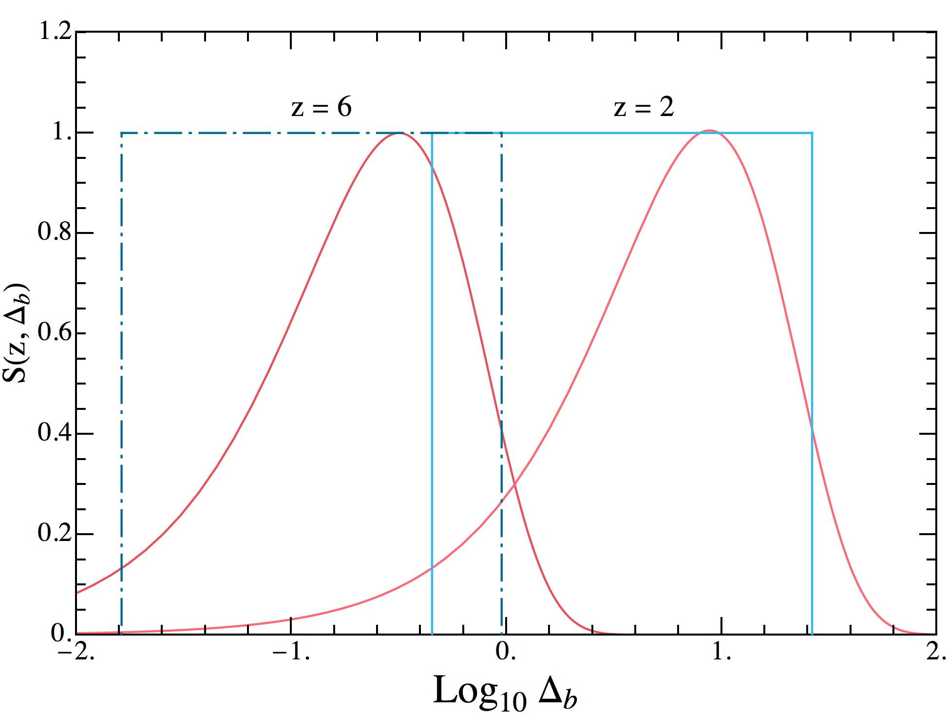
We illustrate the behavior of the suppression factor in Fig. 3, where we plot the absorption probability of Ly- photons as a function of overdensity for various redshifts. Interestingly, Fig. 3 shows that for redshifts when , and thus that Ly- observations are effectively insensitive to energy injection in halos. We conclude that constraints on dark photons with masses larger than or much smaller than will be heavily suppressed.
Using Eq. (26) and Eq. (22), we extend the constraints obtained in Ref. McDermott:2019lch to account for the presence of inhomogeneous structure, both for resonant and non-resonant absorption. This is done by requiring that the observable energy injected given in Eq. (26) is equal to 0.5 eV / baryon in the interval . These constraints are shown in Fig. 444 4 We do not show bounds derived from black hole superradiance Baryakhtar:2017ngi, which in principle can be used to constrain ultralight dark photons with masses near this range, as the existence of such bounds is model dependent Agrawal:2018vin., assuming the sensitivity functions are given as in Eq. (28) (assumed to be the default sensitivity) and Eq. (27) (dubbed ‘Flat window’). For the default sensitivity function, we also show the effect of increasing the integration from to ; the difference is negligible everywhere except the low- tail. Note that Ref. Caputo:2020bdy recently performed a similar analysis, however reached a rather different result – we make a detailed comparison of the two approaches in App. A. In the right panel of Fig. 4 we plot the bounds from non-resonant absorption in both the homogeneous and inhomogeneous limit, assuming either (dashed) or is given by Eq. (28). We see that the effect of structure and the sensitivity function have a minimal effect on the net sensitivity of the non-resonant absorption bounds.
4 21cm Cosmology
The field of 21cm cosmology aims to understand the spatiotemporal evolution of neutral hydrogen in the Universe by studying the hyperfine transition between the ground and first excited state (this is also known as the “21cm” transition). The goal, simply put, is to measure the evolution of the intensity of the redshifted 21cm line; the frequency of an observed line provides direct information on the epoch at which the absorption or emission took place, and the intensity provides various pieces of information on the state of neutral hydrogen, such as its temperature, number density, line-of-sight velocity, and ionization fraction. We review the basics of 21cm cosmology below, but refer the interested reader to Refs. Madau:1996cs; Furlanetto:2006jb; Pritchard:2011xb for more extensive reviews.
The amount of absorption or emission of the gas is determined by the relative occupation number of the ground and excited states, a quantity which is typically parameterized with the so-called spin temperature , defined via
| (34) |
where and represent the excited and ground state, the factor of 3 is the degeneracy factor the excited state, and . Focusing our attention on neutral hydrogen in the IGM during the dark ages, only a small number of processes are capable of changing the ratio of ground and excited states, or equivalently of changing the spin temperature. These are: spontaneous emission, stimulated absorption/emission, collisional excitation/de-excitation, and indirect excitation/de-excitation via Ly- pumping. The spin temperature can be expressed in terms of effective coupling coefficients that characterize the efficiency of each of these processes, the temperature of the background radiation , and the (kinetic) temperature of matter , as
| (35) |
The collisional and Ly- couplings ( and , respectively) are positive semi-definite quantities whose definitions can be found in e.g. Ref. Mena:2019nhm.
Radio experiments searching for the redshifted 21cm line are only sensitive to the relative difference between the intensity produced by these transitions and radio background, which is expected to be dominated by photons in the Rayleigh-Jeans tail of CMB blackbody. As such, the signal is typically expressed as a differential measurement relative to the CMB intensity. Following the convention in radio astronomy to work with effective brightness temperatures rather than intensity itself (the two are directly related by the Rayleigh-Jeans limit of the blackbody relation), the 21cm signal (i.e. the differential brightness temperature) can be expressed as
| (36) |
where is the optical depth of the 21cm line. Since the optical depth is small, the exponential term can be expanded, yielding a differential brightness temperature along a line of sight equal to
| (37) |
where is the neutral hydrogen fraction. It is clear in Eq. (37) that the differential brightness temperature will be seen in emission (i.e. ) if and absorption (i.e. ) if . Furthermore, from Eq. (35) one can see that the spin temperature is bounded to be between the temperature of the CMB and the matter temperature. An immediate consequence is that, if the 21cm signal is observed in absorption (as is expected for ), one can immediately infer that and constrain the maximum temperature of the IGM by taking in Eq. (37). We devote the remainder of this section to investigating the extent to which future 21cm experiments can constrain the heating induced by dark photons should they observe the 21cm signal in absorption.
The simplest and least expensive 21cm experiments are comprised of single antennas that attempt to measure the sky-averaged differential brightness temperature. Recently, the EDGES collaboration Bowman:2018yin claimed the first detection of the global 21cm differential brightness temperature. At the moment, the validity of this measurement is still a matter of hot debate due the complicated nature of foreground removal and its incompatibility with the CDM prediction. Consequently, in this work we will assume that the true 21cm differential brightness temperature is as yet unknown. In the near future, radio interferometers such as HERA55 5 https://reionization.org/ Beardsley:2014bea; DeBoer:2016tnn and SKA66 6 https://www.skatelescope.org/ Mellema:2012ht will measure the 21cm power spectrum from reionization to redshifts as high as . Radio interferometers have a clear advantage over single dish antennas in that smooth radio backgrounds contribute only to low multipoles, which are easy to remove. In addition, the power spectrum contains far more information than the differential brightness temperature, and thus can be a more powerful tool in constraining exotic physics. Incorporating the effect of inhomogeneous energy injection from dark photons in this case is, however, rather involved, and thus we postpone this to future work. In this study, we instead focus on the globally averaged differential brightness temperature (similar sensitivity estimates have been made using the average differential brightness temperature in the homogeneous limit in Ref. Kovetz:2018zes).
Generalizing Eq. (37), we can account for the presence of inhomogeneities in the globally averaged differential brightness temperature Villanueva-Domingo:2019ysf:
| (38) |
where we have included the explicit dependence of the spin temperature on the redshift and over-density. Since we are interested in determining the maximal level of absorption, we can make the substitution , which in most cases will be an overly conservative estimate (see e.g. Ref. Witte:2018itc to understand the expected contribution of x-ray heating by stellar sources). We can then solve for the evolution of the matter temperature at each possible overdensity using
| (39) |
where is the heating rate per unit volume (which includes e.g. x-ray heating and Compton cooling as well as dark photon heating). We adopt initial conditions (which reproduces the solution that when only adiabatic cooling is relevant Villanueva-Domingo:2019ysf), where is the mean adiabatic temperature. In solving Eq. (39) we neglect the term proportional to , since we are focusing on the epoch prior to reionization where the free electron fraction is slowly changing. We also neglect the term proportional to , as this term for typical overdensities is expected to be small relative to to the contribution of adiabatic cooling. We do explicitly include the Compton cooling contribution in the right hand side of Eq. (39), as well as the exotic energy injection from resonant conversion.
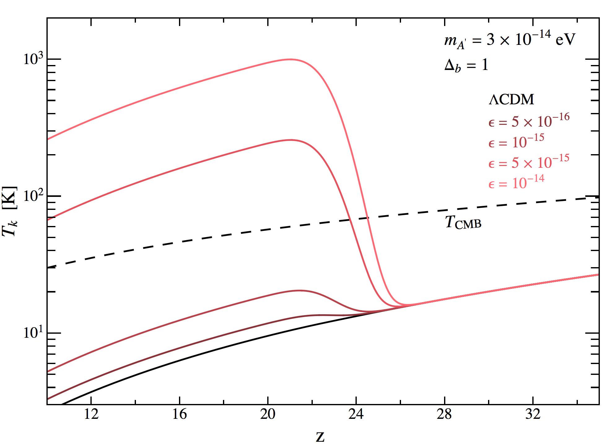
In Fig. 5 we show the evolution of matter temperature relative to that of CDM and to the CMB temperature for dark photons which undergo resonance at high (left) and low (right) redshift. For the high redshift resonance, we solve this using Recfast++ Seager:1999bc; Chluba:2010ca (including a contribution from collisional ionization as in Refs. matsuda1971dissipation; dopita2013astrophysics; McDermott:2019lch), while at low redshift we solve Eq. (39) for . For high redshift resonances (left panel), it is difficult to significantly elevate the matter temperature above that of the CMB during the epoch for which 21cm observations will soon exist. This is because if one heats the medium above the threshold for collisional ionization K, the cooling rate of the medium changes and the net heating saturates. The right panel shows that at late times the story is quite different. One can easily heat the medium above the CMB without encountering any issue with the ionization threshold.

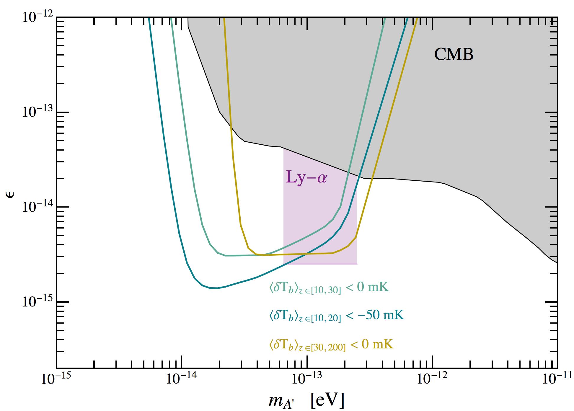
In order to project potential sensitivity of 21cm experiments measuring the global brightness temperature to dark photon dark matter, we adopt two potential experimental configurations, one consistent with an SKA-like experiment Mellema:2012ht and the other being a lunar-based radio array Burns:2011wf; Greenhill:2012mn; Koopmans:2019wbn. We assume that these experiments measure absorption at the level of mK or mK across a range of redshifts. The model is assumed to be falsifiable if the dark photon heats the medium above this level at all points in this redshift range. In reality, constraints may be significantly stronger than this, but such a statement would rely on complicated astrophysical modeling at high redshift where little is currently known. Potential future sensitivity are illustrated in Fig. 6. This shows that 21cm observations could be extremely useful in extending sensitivity to lower-mass dark photons.
Finally, it is worth mentioning that near-future radio interferometers will hope to move well beyond the globally averaged differential brightness temperature and measure the 21cm power spectrum. Far more information is contained in the evolution of the power spectrum than in the global signal, particularly when energy injection proceeds in a largely inhomogeneous way. Consequently, radio interferometers will provide a great opportunity to probe the existence of dark photon dark matter.
5 Discussion
In this section we comment on a number of additional signatures and features that may appear in this model. In particular we discuss the expectations for resonant conversion during the epoch of reionization, potential implications for star formation rates, expected modifications due to bounds derived from the CMB optical depth, and late-time -type spectral distortions due to excess heating of the IGM.
5.1 Reionization
The epoch of reionization refers to the period during which the Universe evolved from being predominately neutral to fully ionized. Measurements of the Gunn-Peterson trough in the spectrum of quasars provide convincing evidence that reionization had completed by Fan:2005es. On the other hand, the integrated optical depth of the CMB measured by Planck Aghanim:2018eyx does not allow for significant changes to the free electron fraction at Heinrich:2016ojb; Hazra:2017gtx; Villanueva-Domingo:2017ahx. Between these epochs, UV radiation (likely) sourced from the first collapsed objects is expected to permeate the Universe and rapidly change the free electron fraction. Understanding how this process began and evolved is currently an active area of research. Still, there are some features which appear consistent among leading theories: namely, the ionizing photons were likely produced in over-densities and had relatively short mean free paths in the neutral media that they were ionizing. Consequently, to first order one can imagine that reionization proceeded via the formation of ionized bubbles, inside of which the Universe is fully ionized (with ), while the IGM outside the bubbles remained nearly unaffected. The free electron fraction outside of the ionized bubbles would be given by the pre-reionization value Furlanetto:2005xx; Zahn:2006sg; McQuinn:2006et; Mesinger:2007pd, until the bubbles grow and merge, at which point reionization is complete.
The dramatically inhomogeneous nature of reionization has implications for resonant dark photon conversion, since the inhomogeneous structure of complicates the spatial and temporal understanding of the resonance. Naively, one may be tempted to use the globally averaged value of the free electron fraction to understand which dark photon masses allow for resonant conversion during the reionization epoch. Unfortunately this is wrong since reionization is an intrinsically inhomogeneous process. A better attempt at treating the Universe during this epoch is to work in a two-phase approximation, i.e. assuming the co-existence of a fully ionized medium with a medium whose ionization level is consistent with the standard background evolution (without reionization sources), and neglect the boundaries between ionized and non-ionized regions. We believe that this is a reasonable approximation given the short mean free path of the ionizing photons in the neutral medium. The question then becomes: how should one map over-densities to ionized and non-ionized regions?
Here, we briefly sketch two possibilities for approximating the effect of energy injection from resonant dark photon conversion during this epoch. However, given the large theoretical uncertainties associated to modeling reionization, the constraints obtained in this section should not be interpreted as robust. Instead, this discussion is intended merely as an exercise to illustrate how considering inhomogeneities in during the epoch of reionization might affect the bounds derived elsewhere.
Adopting the two phase approximation, and assuming we have a measurement of the global free electron fraction, one can estimate what volumetric fraction of the Universe is ionized via
| (40) |
where and is the value of the free electron fraction assuming ionization has not modified the evolution of the IGM. The simplest assumption one can make is that under-densities and over-densities are equally likely to be ionized. This amounts to a differential rate of energy injection of
| (41) |
Here, the notation means that the resonant redshift in Eq. (14) is determined with a particular value of the free electron fraction. We will refer to this scenario as the ‘homogeneous’ reionization. As previously mentioned, however, we expect ionizing photons to be produced in collapsed objects, meaning they originate from over-densities and expand outwards. At the converse extreme, we might thus expect ionization to first occur in the densest objects, and proceed from over-densities to under-densities. We will refer to this scenario as the ‘strongly inhomogeneous’ scenario. In this case, we can identify at each redshift the threshold of over-densities defining the boundary between ionized and non-ionized regions by solving
| (42) |
In this case, one can write the differential rate of energy injection
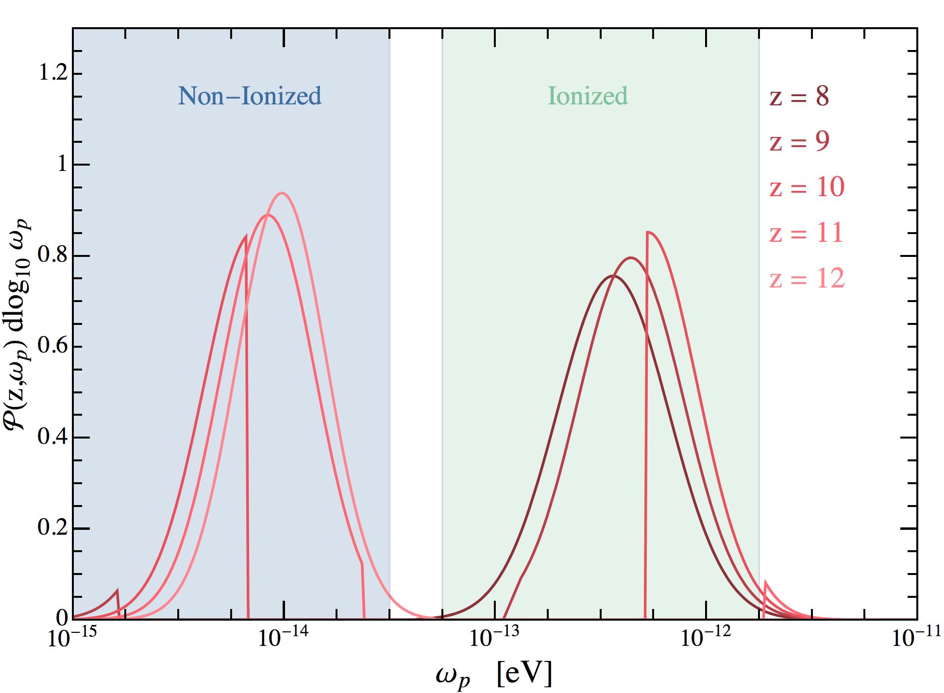
An important consequence of the strongly inhomogeneous scenario is the appearance of a gap in the evolution of the PDF characterizing the plasma frequency of the Universe. This is illustrated in Fig. 7, where we plot the evolution of the PDF characterizing during reionization in the strongly inhomogeneous scenario, assuming the mean free electron fraction is given by a function centered at and of width . We have highlighted the two phases via the labels ‘non-ionized’ and ‘ionized’. The sharp cut in the distributions illustrates the evolution of with time.

For both reionization scenarios discussed, we derive an illustrative ‘bound’ on dark photon dark matter by requiring that the IGM is not over-heated in the redshift range (which would also assume that the temperature evolution of the IGM is well understood, which it is not Gaikwad:2020art). We take the requirement eV/ baryon. We adopt a recent modeling of the mean free electron fraction from Ref. Naidu:2019gvi, which is consistent with high quasar measurements. We plot the bounds obtained for both the homogeneous and strongly inhomogeneous scenarios in Fig. 8. The bounds obtained for are similar, but for smaller masses the difference in these treatments can be significant.
We conclude this section by emphasizing that a detailed treatment of reionization will be needed to move beyond these two extremal examples, and will likely require numerical simulations to understand the correlations between ionized regions and over-densities.
5.2 Star formation
Dark-photon-induced heating may have strong implications for star formation. Since observations of high-redshift star formation do not yet exist, we simply outline here how the star formation rate might be suppressed, and the interesting regions of parameter space which might be testable using observations from 21cm telescopes or the James Webb telescope gardner2006james; stiavelli2009first in the near future.
Star formation is typically expected to be efficient when the kinetic temperature of the gas in a gravitationally bound object exceeds some threshold at which the cooling, and subsequent collapse, of gas becomes efficient. Assuming the kinetic temperature in the halo is approximately given by the virial temperature , one can relate this threshold directly to the host halo mass via Shapiro:1998zp; Mena:2019nhm
| (43) |
We have assumed the neutral hydrogen fraction is given by the IGM value, the halo profile is approximately given by that of a truncated isothermal sphere, and we recall that is the mean molecular weight ( for a neutral medium). The virial overdensity based on spherical collapse is given by Bryan:1997dn
| (44) |
where
| (45) |
Efficient star formation is only expected to proceed in halos with virial temperatures K Evrard:1990fu; blanchard1992origin; Tegmark:1996yt; Haiman:1999mn, as this is the threshold for which molecular hydrogen cooling becomes efficient. While there is uncertainty in both how to treat this threshold and where exactly it lies, it is clear that a sufficient number of collapsed objects with these masses must exist in order to efficiently produce star forming regions.
If dark photon heating is active near the epoch of star formation, however, it may be possible that thermal pressure prevents the formation of star forming halos. That is to say, if the medium is heated to a sufficient degree, the Jeans mass may increase to a level where star forming halos would never have collapsed. To assess the extent to which this may occur, we compute the Jeans mass as a function of redshift and overdensity via
| (46) |
where is the average density in the radius of interest, and the Jeans length is as defined in Sec. 2.2. As before, we will assume that the baryon density approximately follows that of the dark matter, and write . The temperature evolution of a particular overdensity in the presence of dark photon heating is obtained by solving equations for the evolution of the matter temperature as in Sec. 4; thus, given a large-scale overdensity , one can determine the redshift-dependent evolution of the Jeans mass for any dark photon candidate.


We compare in the left panel of Fig. 9 the evolution of the Jeans mass in an overdensity as a function of redshift, assuming a dark photon mass eV and various mixings. We compare this mass scale with the redshift-dependent virial mass , which is obtained by assuming the matter profile is given by a truncated isothermal profile with a temperature of K. Typically, star formation is expected to begin near redshifts , and thus if the Jeans mass sufficiently exceeds over this interval, star formation rates can be dramatically altered. In order to assess the potential impact of dark photons on the star formation rate, we highlight in the right panel of Fig. 9 the dark photon parameter space capable of suppressing star formation, which we define here as those models for which over the entirety of the interval , assuming star formation is observed in an isolated over-density 77 7 Stars in regions with at these redshifts should be extremely rare, and thus we expect the curves near to be the most relevant to future surveys.. This final assumption will likely not be met in most experiments, and in reality one should expect the sensitivity to be something of a -weighted average over these curves. However, if high-redshift 21cm experiments in the distant future find themselves capable of achieving 21cm tomography Madau:1996cs, perhaps the environmental dependence can be isolated. We also emphasize that this could be a detectable signature in the James Webb Space Telescope (JWST) which is likely to come online in the near future gardner2006james; stiavelli2009first.
5.3 Dark Ages Energy Injection
It was shown in Ref. McDermott:2019lch that strong constraints can be derived on dark photons that resonantly convert during the dark ages. Dark photons converting during this epoch will efficiently deposit their energy in baryons, heating the medium above the collisional ionization threshold and subsequently causing the medium to prematurely re-ionize. In the case of a homogeneous Universe, the energy injection is not sustained (i.e. it occurs over a short period of time, after which atoms are allowed to cool), and some atoms will recombine. However, the asymptotic free electron fraction will be significantly larger than in the case of CDM. This can be strongly constrained using the CMB since the optical depth is extremely sensitive to the free electron fraction between recombination and reionization. This bound was recently criticized Caputo:2020bdy, but we argue here that such concerns are unwarranted.
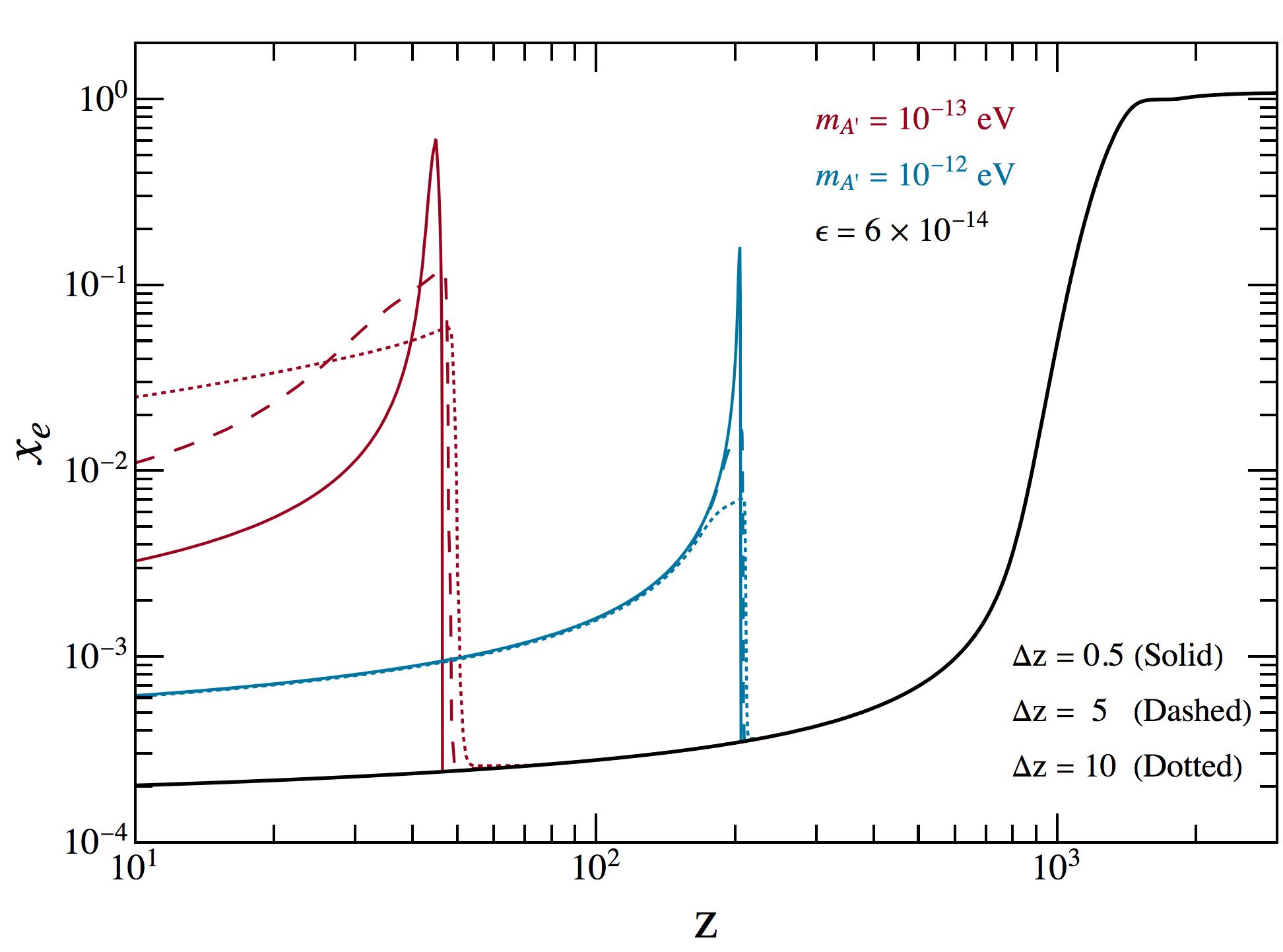
There are two potential causes for concern. The first arises from the fact that the energy injection in Ref. McDermott:2019lch was treated assuming the redshift dependence followed a Gaussian distribution with . From Fig. 1 and Fig. 2 it is clear that the presence of inhomogeneities broadens the energy injection such that it spans at . This concern is easy to address. In Fig. 10 we plot the evolution of the free electron fraction for two different dark photon parameters, assuming the energy injection can be modeled with a Gaussian distribution in redshift with (solid), (dashed), or (dotted). For the high redshift resonance (i.e. large ) there is nearly no difference between all of the curves. At low redshifts, the energy injection actually produces larger asymptotic values of the free electron fraction. The difference between these two sets of curves partially arises from the fact that a value of is large relative to the resonance redshift itself, and partially because the efficiency of cooling processes depends on the maximal level of ionization obtained during the energy injection process (notice that the peak ionization fraction is larger for the narrow Gaussian). Since the energy injection is extremely sensitive to the value of , we expect the differences here to produce tiny changes in the derived limit.
The second concern is related to potential back-reaction. In the case of a homogeneous Universe it was shown that there can be no back-reaction which would cause the resonance to prematurely end McDermott:2019lch. The reason is simply that the resonant timescale is short relative to that of collisional ionization. The case of an inhomogeneous Universe is slightly more complicated, because the resonance timescale is not dictated solely by the width of the resonance, but rather by the rate at which sweeps through the overdensity PDF. However, in order for back-reaction to occur in the inhomogeneous scenario, not only must reionization in some over-density take place on short time scales, but free electrons produced in this process must quickly and efficiently diffuse to larger over-densities. Since the electrons are always non-relativistic, we expect this to be slow relative to the Hubble rate, and therefore we expect back-reaction to be negligible. A proper treatment of this process is beyond the scope of this work, and we leave a detailed exploration of such effects to future studies.
5.4 Late-time Spectral Distortions
It was also shown in Ref. McDermott:2019lch that strong bounds can be placed on dark photon dark matter resonantly converting into photons prior to recombination from the non-observation of spectral distortions in the CMB. Should the gas be heated to a sufficiently high level, type distortions can still be induced after recombination; consequently, it is in general also possible to constrain dark photons from late-time heating of the IGM.
For heating that occurs at redshifts , one would naturally expect constraints from early reionization (discussed in Sec. 5.3) to be much stronger than those arising from late-time spectral distortions. Similarly, one must inject heat into the IGM at a level much greater than eV / baryon for redshifts in order to produce observable spectral distortions, implying Ly- constraints will likely be stronger in this regime. At lower redshifts, one suffers from a vast array of astrophysical and cosmological uncertainty. In addition, the IGM is much hotter, meaning more energy must be injected in order to produce dramatic changes. Perhaps the most promising regime in which to look for these effects is at redshifts near reionization. In CDM, reionization is already expected to contribute to -type spectral distortions at the level of Sunyaev:2013aoa, which is slightly above the expected threshold for a futuristic CMB spectral distortion experiment like PIXIE Kogut:2011xw or PRISIM andre2014prism. In order to heuristically estimate what type of sensitivity these experiments might have to exotic heating from dark photon conversion, we evolve the temperature of the IGM as described in Sec. 4, assuming reionization begins only at (note this is probably a rather optimistic assumption, but is sufficient for illustrative purposes). We then compute the contribution of this heating to the Compton parameter Sunyaev:2013aoa, which when averaged over yields
| (47) |
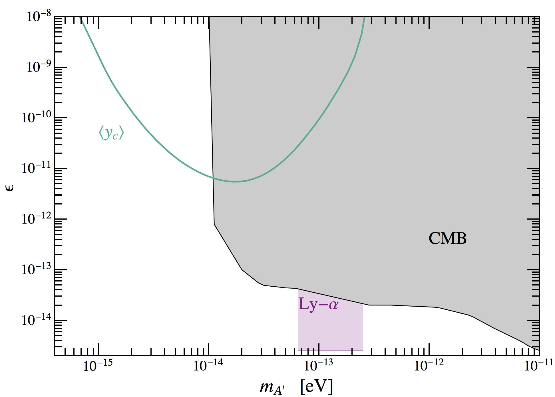
We define this signal to be observable when , although this number should be understood purely as a rough estimate, as uncertainties associated with reionization may alter the CDM expectation by a factor of a few (exploring the detailed degeneracies between reionization histories and exotic energy injection from dark photons is beyond the scope of the current work). We show the sensitivity for a future PIXIE/PRISIM-like experiment in Fig. 11. Depending on the details of reionization, this method may provide a probe of dark photons at masses below eV.
6 Conclusion
In this work we have investigated the extent to which inhomogeneous structure can alter the cosmology of an ultra-light dark photon dark matter that injects energy after the formation of the CMB. This generalizes and expands upon existing work McDermott:2019lch, revisiting the robustness of existing bounds and investigating novel signatures which may be particularly sensitive to the inhomogeneous features arising at . Accounting for inhomogeneities has important implications for dark photons capable of resonantly converting to visible photons, since the resonance occurs when the dark photon mass equals the local plasma frequency of the ambient medium. Consequently, the homogeneous Universe approximation assumes (up to effects associated with reionization) a one-to-one mapping between the redshift of the resonance and the dark photon mass, while inhomogeneous structure at e.g. may produce resonant conditions for dark photons with masses spanning multiple orders of magnitude. The implications are most prominent for dark photons with lower masses, as such particles may appear to have no chance to undergo resonance in the homogeneous approximation, but in reality can resonantly convert in (and thus inject energy into) cosmic voids.
Using current observations of the Ly- forest, we derived constraints in Sec. 3 on the excess heating of the IGM, extending on the work of Ref. McDermott:2019lch which had neglected the presence of inhomogeneities. Accounting for the presence of structure allows us to extend these constraints to masses approximately an order of magnitude smaller than were obtained in the homogeneous approximation, with only minor (but real) corrections to the constraining power obtained in the homogeneous limit. We found that the ability to constrain larger masses, however, was severely limited by the fact that quasar fluxes are preferentially absorbed in overdensities.
In Sec. 4 we investigated the extent to which future radio observations of the 21cm absorption signal at high redshift might be able to constrain resonant dark photon conversion. By conservatively assuming that future experiments observe the signal in absorption, which is a generic expectation for , we show that experiments might be able to constrain mixings at the level of for eV. We expect that radio interferometers looking to measure the 21cm power spectrum will significantly improve the projected sensitivity of 21cm observations to light dark photons. Due to the complexity of modeling the contribution of inhomogeneous dark photon heating to the 21cm power spectrum, we defer a complete treatment of observables from this epoch to future work.
Lastly, we have commented on other signatures that may arise at late times. In particular, we have discussed the epoch of reionization and the complications associated with understanding the distribution and evolution of plasma frequencies. In this case, we have shown that future data should allow one to study exotic energy injection during reionization, but robust analysis will require a detailed understanding of spatial inhomogeneities of ionized and non-ionized regions. We have also commented on the extent to which localized heating produced from dark photon absorption can increase the Jeans mass – we have shown that efficient heating may actually raise the Jeans mass above the star forming threshold, particularly in under-densities, significantly suppressing star formation rates in these regions. Such effects may potentially be observable with the James Webb telescope or using 21cm tomography. Finally, we have shown that future experiments like PIXIE or PRISIM (which hope to measure spectral distortions in the CMB) may be sensitive to the heating of the IGM at redshifts just prior to reionization, potentially gaining unprecedented sensitivity to dark photons with masses eV.
In summary, properly accounting for the existence of baryonic structure at is crucial for understanding the extent to which cosmology can probe the existence of ultra-light dark photon dark matter. The predominant effect of including these inhomogeneities is that it makes cosmological observations sensitive to a wider range of masses, allowing to probe lower masses, while relaxing some constraints at larger mass. Furthermore, we emphasize that experiments which themselves are inherently sensitive to the inhomogeneous state of the Universe could provide striking signatures that are unique to light dark photon dark matter, and thus offer a tantalizing opportunity for a positive detection, should they exist.
Acknowledgements.
We thank Nick Gnedin, Hongwan Liu, Josh Ruderman, Andrea Caputo, and Siddarth Mishra-Sharma for discussions. SJW thanks Luisa Lucie-Smith and Andreu Font-Ribera for their valuable discussions on structure formation and the Lyman forest, respectively. SJW and SR acknowledge support from the European Union’s Horizon 2020 research and innovation program under the Marie Skłodowska-Curie grant agreements No. 690575 and 674896. SJW acknowledges support under Spanish grants FPA2014-57816-P and FPA2017-85985-P of the MINECO and PROMETEO II/2014/050 of the Generalitat Valenciana. SR also acknowledges support from the “Spanish Agencia Estatal de Investigación” (AEI) and the EU “Fondo Europeo de Desarrollo Regional” (FEDER) through the project FPA2016-78645-P; and through the Centro de Excelencia Severo Ochoa Program under grant SEV-2016-0597. Fermilab is operated by Fermi Research Alliance, LLC under Contract No. DE-AC02-07CH11359 with the United States Department of Energy.References
- (1) D. J. E. Marsh, Axion Cosmology, Phys. Rept. 643 (2016) 1–79, [1510.07633].
- (2) I. G. Irastorza and J. Redondo, New experimental approaches in the search for axion-like particles, Prog. Part. Nucl. Phys. 102 (2018) 89–159, [1801.08127].
- (3) J. Jaeckel, J. Redondo and A. Ringwald, Signatures of a hidden cosmic microwave background, Phys. Rev. Lett. 101 (2008) 131801, [0804.4157].
- (4) M. Pospelov, A. Ritz and M. B. Voloshin, Bosonic super-WIMPs as keV-scale dark matter, Phys. Rev. D78 (2008) 115012, [0807.3279].
- (5) J. Redondo and M. Postma, Massive hidden photons as lukewarm dark matter, JCAP 0902 (2009) 005, [0811.0326].
- (6) A. Mirizzi, J. Redondo and G. Sigl, Microwave Background Constraints on Mixing of Photons with Hidden Photons, JCAP 0903 (2009) 026, [0901.0014].
- (7) A. E. Nelson and J. Scholtz, Dark Light, Dark Matter and the Misalignment Mechanism, Phys. Rev. D84 (2011) 103501, [1105.2812].
- (8) P. Arias, D. Cadamuro, M. Goodsell, J. Jaeckel, J. Redondo and A. Ringwald, WISPy Cold Dark Matter, JCAP 1206 (2012) 013, [1201.5902].
- (9) P. W. Graham, J. Mardon and S. Rajendran, Vector Dark Matter from Inflationary Fluctuations, Phys. Rev. D93 (2016) 103520, [1504.02102].
- (10) S. Dubovsky and G. Hernndez-Chifflet, Heating up the Galaxy with Hidden Photons, JCAP 1512 (2015) 054, [1509.00039].
- (11) P. Agrawal, N. Kitajima, M. Reece, T. Sekiguchi and F. Takahashi, Relic Abundance of Dark Photon Dark Matter, 1810.07188.
- (12) J. A. Dror, K. Harigaya and V. Narayan, Parametric Resonance Production of Ultralight Vector Dark Matter, Phys. Rev. D99 (2019) 035036, [1810.07195].
- (13) R. T. Co, A. Pierce, Z. Zhang and Y. Zhao, Dark Photon Dark Matter Produced by Axion Oscillations, Phys. Rev. D99 (2019) 075002, [1810.07196].
- (14) M. Bastero-Gil, J. Santiago, L. Ubaldi and R. Vega-Morales, Vector dark matter production at the end of inflation, JCAP 1904 (2019) 015, [1810.07208].
- (15) A. Bhoonah, J. Bramante, F. Elahi and S. Schon, Galactic Center gas clouds and novel bounds on ultralight dark photon, vector portal, strongly interacting, composite, and super-heavy dark matter, Phys. Rev. D100 (2019) 023001, [1812.10919].
- (16) E. D. Kovetz, I. Cholis and D. E. Kaplan, Bounds on ultralight hidden-photon dark matter from observation of the 21 cm signal at cosmic dawn, Phys. Rev. D99 (2019) 123511, [1809.01139].
- (17) A. J. Long and L.-T. Wang, Dark Photon Dark Matter from a Network of Cosmic Strings, Phys. Rev. D99 (2019) 063529, [1901.03312].
- (18) G. Alonso-Álvarez, T. Hugle and J. Jaeckel, Misalignment and Co.: (Pseudo-)scalar and vector dark matter with curvature couplings, 1905.09836.
- (19) K. Nakayama, Vector Coherent Oscillation Dark Matter, 1907.06243.
- (20) D. Wadekar and G. R. Farrar, First direct astrophysical constraints on dark matter interactions with ordinary matter at very low velocities, 1903.12190.
- (21) S. D. McDermott and S. J. Witte, The Cosmological Evolution of Light Dark Photon Dark Matter, Phys. Rev. D101 (2020) 063030, [1911.05086].
- (22) A. Caputo, H. Liu, S. Mishra-Sharma and J. T. Ruderman, Dark Photon Oscillations in Our Inhomogeneous Universe, 2002.05165.
- (23) B. Holdom, Two U(1)’s and Epsilon Charge Shifts, Phys. Lett. 166B (1986) 196–198.
- (24) B. Himmetoglu, C. R. Contaldi and M. Peloso, Instability of anisotropic cosmological solutions supported by vector fields, Phys. Rev. Lett. 102 (2009) 111301, [0809.2779].
- (25) B. Himmetoglu, C. R. Contaldi and M. Peloso, Ghost instabilities of cosmological models with vector fields nonminimally coupled to the curvature, Phys. Rev. D80 (2009) 123530, [0909.3524].
- (26) M. Karciauskas and D. H. Lyth, On the health of a vector field with (R A2)/6 coupling to gravity, JCAP 1011 (2010) 023, [1007.1426].
- (27) J. D. Bowman, A. E. E. Rogers, R. A. Monsalve, T. J. Mozdzen and N. Mahesh, An absorption profile centred at 78 megahertz in the sky-averaged spectrum, Nature 555 (2018) 67–70.
- (28) M. Pospelov, J. Pradler, J. T. Ruderman and A. Urbano, Room for New Physics in the Rayleigh-Jeans Tail of the Cosmic Microwave Background, Phys. Rev. Lett. 121 (2018) 031103, [1803.07048].
- (29) K. Bondarenko, J. Pradler and A. Sokolenko, Constraining dark photons and their connection to 21 cm cosmology with CMB data, 2002.08942.
- (30) A. A. Garcia, K. Bondarenko, S. Ploeckinger, J. Pradler and A. Sokolenko, Effective photon mass and (dark) photon conversion in the inhomogeneous Universe, 2003.10465.
- (31) C. Zener, Nonadiabatic crossing of energy levels, Proc. Roy. Soc. Lond. A137 (1932) 696–702.
- (32) H. An, M. Pospelov and J. Pradler, New stellar constraints on dark photons, Phys. Lett. B725 (2013) 190–195, [1302.3884].
- (33) J. H. Chang, R. Essig and S. D. McDermott, Revisiting Supernova 1987A Constraints on Dark Photons, JHEP 01 (2017) 107, [1611.03864].
- (34) E. Aver, K. A. Olive and E. D. Skillman, The effects of He I 10830 on helium abundance determinations, JCAP 1507 (2015) 011, [1503.08146].
- (35) C. Pitrou, A. Coc, J.-P. Uzan and E. Vangioni, Precision big bang nucleosynthesis with improved Helium-4 predictions, Phys. Rept. 754 (2018) 1–66, [1801.08023].
- (36) B. D. Fields, K. A. Olive, T.-H. Yeh and C. Young, Big-Bang Nucleosynthesis After Planck, JCAP 2003 (2020) 010, [1912.01132].
- (37) D. J. Fixsen, The Temperature of the Cosmic Microwave Background, Astrophys. J. 707 (2009) 916–920, [0911.1955].
- (38) P. Coles and B. Jones, A Lognormal model for the cosmological mass distribution, Mon. Not. Roy. Astron. Soc. 248 (1991) 1–13.
- (39) F. Bernardeau and L. Kofman, Properties of the cosmological density distribution function, Astrophys. J. 443 (1995) 479–498, [astro-ph/9403028].
- (40) I. Kayo, A. Taruya and Y. Suto, Probability distribution function of cosmological density fluctuations from Gaussian initial condition: comparison of one- and two-point log-normal model predictions with n-body simulations, Astrophys. J. 561 (2001) 22–34, [astro-ph/0105218].
- (41) D. Nelson et al., The IllustrisTNG Simulations: Public Data Release, 1812.05609.
- (42) S. McAlpine et al., The EAGLE simulations of galaxy formation: public release of halo and galaxy catalogues, Astron. Comput. 15 (2016) 72–89, [1510.01320].
- (43) I. G. McCarthy, J. Schaye, S. Bird and A. M. C. Le Brun, The BAHAMAS project: Calibrated hydrodynamical simulations for large-scale structure cosmology, Mon. Not. Roy. Astron. Soc. 465 (2017) 2936–2965, [1603.02702].
- (44) S. Genel, M. Vogelsberger, V. Springel, D. Sijacki, D. Nelson, G. Snyder et al., Introducing the Illustris Project: the evolution of galaxy populations across cosmic time, Mon. Not. Roy. Astron. Soc. 445 (2014) 175–200, [1405.3749].
- (45) S. Foreman, W. Coulton, F. Villaescusa-Navarro and A. Barreira, Baryonic effects on the matter bispectrum, 1910.03597.
- (46) M. P. van Daalen, I. G. McCarthy and J. Schaye, Exploring the effects of galaxy formation on matter clustering through a library of simulation power spectra, Mon. Not. Roy. Astron. Soc. 491 (2020) 2424–2446, [1906.00968].
- (47) M. M. Ivanov, A. A. Kaurov and S. Sibiryakov, Non-perturbative probability distribution function for cosmological counts in cells, JCAP 1903 (2019) 009, [1811.07913].
- (48) P. Valageas, Dynamics of gravitational clustering. 2. Steepest-descent method for the quasi-linear regime, Astron. Astrophys. 382 (2002) 412, [astro-ph/0107126].
- (49) P. Valageas, Dynamics of gravitational clustering v. subleading corrections in the quasi-linear regime, Astron. Astrophys. 382 (2002) 477, [astro-ph/0109408].
- (50) D. Blas, J. Lesgourgues and T. Tram, The Cosmic Linear Anisotropy Solving System (CLASS) II: Approximation schemes, JCAP 1107 (2011) 034, [1104.2933].
- (51) R. Takahashi, M. Sato, T. Nishimichi, A. Taruya and M. Oguri, Revising the Halofit Model for the Nonlinear Matter Power Spectrum, Astrophys. J. 761 (2012) 152, [1208.2701].
- (52) H. Mo, F. Van den Bosch and S. White, Galaxy formation and evolution. Cambridge University Press, 2010.
- (53) X.-H. Fan, M. A. Strauss, R. H. Becker, R. L. White, J. E. Gunn, G. R. Knapp et al., Constraining the evolution of the ionizing background and the epoch of reionization with z 6 quasars. 2. a sample of 19 quasars, Astron. J. 132 (2006) 117–136, [astro-ph/0512082].
- (54) C. H. Heinrich, V. Miranda and W. Hu, Complete Reionization Constraints from Planck 2015 Polarization, Phys. Rev. D95 (2017) 023513, [1609.04788].
- (55) D. K. Hazra and G. F. Smoot, Witnessing the reionization history using Cosmic Microwave Background observation from Planck, JCAP 1711 (2017) 028, [1708.04913].
- (56) P. Villanueva-Domingo, S. Gariazzo, N. Y. Gnedin and O. Mena, Was there an early reionization component in our universe?, JCAP 1804 (2018) 024, [1712.02807].
- (57) M. McQuinn, The Evolution of the Intergalactic Medium, Ann. Rev. Astron. Astrophys. 54 (2016) 313–362, [1512.00086].
- (58) P. R. U. Sanderbeck, A. D’Aloisio and M. J. McQuinn, Models of the Thermal Evolution of the Intergalactic Medium After Reionization, Mon. Not. Roy. Astron. Soc. 460 (2016) 1885–1897, [1511.05992].
- (59) J. Oñorbe, J. F. Hennawi and Z. Lukić, Self-consistent modeling of reionization in cosmological hydrodynamical simulations, The Astrophysical Journal 837 (2017) 106.
- (60) M. Walther, J. Onorbe, J. F. Hennawi and Z. Lukic, New Constraints on IGM Thermal Evolution from the Ly- Forest Power Spectrum, Astrophys. J. 872 (2019) 13, [1808.04367].
- (61) P. Gaikwad et al., Probing the thermal state of the intergalactic medium at with the transmission spikes in high-resolution Ly forest spectra, 2001.10018.
- (62) S. E. I. Bosman, X. Fan, L. Jiang, S. L. Reed, Y. Matsuoka, G. D. Becker et al., New constraints on Lyman- opacity with a sample of 62 quasarsat z ¿ 5.7, Mon. Not. Roy. Astron. Soc. 479 (2018) 1055–1076, [1802.08177].
- (63) G. D. Becker, J. S. Bolton, M. G. Haehnelt and W. L. W. Sargent, Detection of Extended He II Reionization in the Temperature Evolution of the Intergalactic Medium, Mon. Not. Roy. Astron. Soc. 410 (2011) 1096, [1008.2622].
- (64) Z. Lukić, C. W. Stark, P. Nugent, M. White, A. A. Meiksin and A. Almgren, The Lyman- forest in optically thin hydrodynamical simulations, Mon. Not. Roy. Astron. Soc. 446 (2015) 3697–3724, [1406.6361].
- (65) P. U. Sanderbeck and S. Bird, Inhomogeneous heii reionization in hydrodynamic simulations, arXiv preprint arXiv:2002.05733 (2020) .
- (66) M. Baryakhtar, R. Lasenby and M. Teo, Black Hole Superradiance Signatures of Ultralight Vectors, Phys. Rev. D96 (2017) 035019, [1704.05081].
- (67) P. Madau, A. Meiksin and M. J. Rees, 21-CM tomography of the intergalactic medium at high redshift, Astrophys. J. 475 (1997) 429, [astro-ph/9608010].
- (68) S. Furlanetto, S. P. Oh and F. Briggs, Cosmology at Low Frequencies: The 21 cm Transition and the High-Redshift Universe, Phys. Rept. 433 (2006) 181–301, [astro-ph/0608032].
- (69) J. R. Pritchard and A. Loeb, 21-cm cosmology, Rept. Prog. Phys. 75 (2012) 086901, [1109.6012].
- (70) O. Mena, S. Palomares-Ruiz, P. Villanueva-Domingo and S. J. Witte, Constraining the primordial black hole abundance with 21-cm cosmology, Phys. Rev. D100 (2019) 043540, [1906.07735].
- (71) A. P. Beardsley, M. F. Morales, A. Lidz, M. Malloy and P. M. Sutter, Adding Context to James Webb Space Telescope Surveys with Current and Future 21cm Radio Observations, Astrophys. J. 800 (2015) 128, [1410.5427].
- (72) D. R. DeBoer et al., Hydrogen Epoch of Reionization Array (HERA), Publ. Astron. Soc. Pac. 129 (2017) 045001, [1606.07473].
- (73) G. Mellema et al., Reionization and the Cosmic Dawn with the Square Kilometre Array, Exper. Astron. 36 (2013) 235–318, [1210.0197].
- (74) P. Villanueva-Domingo, O. Mena and J. Miralda-Escudé, On the maximum amplitude of the high-redshift 21-cm absorption feature, 1912.09488.
- (75) S. Witte, P. Villanueva-Domingo, S. Gariazzo, O. Mena and S. Palomares-Ruiz, EDGES result versus CMB and low-redshift constraints on ionization histories, Phys. Rev. D97 (2018) 103533, [1804.03888].
- (76) S. Seager, D. D. Sasselov and D. Scott, A new calculation of the recombination epoch, Astrophys. J. 523 (1999) L1–L5, [astro-ph/9909275].
- (77) J. Chluba and R. M. Thomas, Towards a complete treatment of the cosmological recombination problem, Mon. Not. Roy. Astron. Soc. 412 (2011) 748, [1010.3631].
- (78) T. Matsuda, H. Sato and H. Takeda, Dissipation of primordial turbulence and thermal history of the universe, Progress of Theoretical Physics 46 (1971) 416–432.
- (79) M. A. Dopita and R. S. Sutherland, Astrophysics of the diffuse universe. Springer Science & Business Media, 2013.
- (80) J. O. Burns, T. J. W. Lazio, S. D. Bale, J. D. Bowman, R. F. Bradley, C. L. Carilli et al., Probing the First Stars and Black Holes in the Early Universe with the Dark Ages Radio Explorer (DARE), Adv. Space Res. 49 (2012) 433–450, [1106.5194].
- (81) L. J. Greenhill and G. Bernardi, HI Epoch of Reionization Arrays, 1201.1700.
- (82) L. Koopmans et al., Peering into the Dark (Ages) with Low-Frequency Space Interferometers: Using the 21-cm signal of Neutral Hydrogen from the Infant Universe to probe Fundamental (Astro)Physics, 1908.04296.
- (83) Planck collaboration, N. Aghanim et al., Planck 2018 results. VI. Cosmological parameters, 1807.06209.
- (84) S. R. Furlanetto and S. P. Oh, Taxing the rich: Recombinations and bubble growth during reionization, Mon. Not. Roy. Astron. Soc. 363 (2005) 1031–1048, [astro-ph/0505065].
- (85) O. Zahn, A. Lidz, M. McQuinn, S. Dutta, L. Hernquist, M. Zaldarriaga et al., Simulations and Analytic Calculations of Bubble Growth During Hydrogen Reionization, Astrophys. J. 654 (2006) 12–26, [astro-ph/0604177].
- (86) M. McQuinn, A. Lidz, O. Zahn, S. Dutta, L. Hernquist and M. Zaldarriaga, The Morphology of HII Regions during Reionization, Mon. Not. Roy. Astron. Soc. 377 (2007) 1043–1063, [astro-ph/0610094].
- (87) A. Mesinger and S. Furlanetto, Efficient Simulations of Early Structure Formation and Reionization, Astrophys. J. 669 (2007) 663, [0704.0946].
- (88) R. P. Naidu, S. Tacchella, C. A. Mason, S. Bose, P. A. Oesch and C. Conroy, Rapid Reionization by the Oligarchs: The Case for Massive, UV-Bright, Star-Forming Galaxies with High Escape Fractions, 1907.13130.
- (89) J. P. Gardner, J. C. Mather, M. Clampin, R. Doyon, M. A. Greenhouse, H. B. Hammel et al., The james webb space telescope, Space Science Reviews 123 (2006) 485–606.
- (90) M. Stiavelli, J. Mather, M. Clampin, R. Doyon, K. Flanagan, M. Franx et al., First light and reionization: open questions in the post-jwst era, astro2010: The Astronomy and Astrophysics Decadal Survey 2010 (2009) .
- (91) P. R. Shapiro and I. T. Iliev, A Model for the postcollapse equilibrium of cosmological structure: truncated isothermal spheres from top-hat density perturbations, Mon. Not. Roy. Astron. Soc. 307 (1999) 203, [astro-ph/9810164].
- (92) G. L. Bryan and M. L. Norman, Statistical properties of x-ray clusters: Analytic and numerical comparisons, Astrophys. J. 495 (1998) 80, [astro-ph/9710107].
- (93) A. E. Evrard, Formation and evolution of X-ray clusters - A hydrodynamic simulation of the intracluster medium, Astrophys. J. 363 (1990) 349–366.
- (94) A. Blanchard, D. Valls-Gabaud and G. Mamon, The origin of the galaxy luminosity function and the thermal evolution of the intergalactic medium, Astronomy and Astrophysics 264 (1992) 365–378.
- (95) M. Tegmark, J. Silk, M. J. Rees, A. Blanchard, T. Abel and F. Palla, How small were the first cosmological objects?, Astrophys. J. 474 (1997) 1–12, [astro-ph/9603007].
- (96) Z. Haiman, T. Abel and M. J. Rees, The radiative feedback of the first cosmological objects, Astrophys. J. 534 (2000) 11–24, [astro-ph/9903336].
- (97) R. A. Sunyaev and R. Khatri, Unavoidable CMB spectral features and blackbody photosphere of our Universe, Int. J. Mod. Phys. D 22 (2013) 1330014, [1302.6553].
- (98) A. Kogut et al., The Primordial Inflation Explorer (PIXIE): A Nulling Polarimeter for Cosmic Microwave Background Observations, JCAP 07 (2011) 025, [1105.2044].
- (99) P. André, C. Baccigalupi, A. Banday, D. Barbosa, B. Barreiro, J. Bartlett et al., Prism (polarized radiation imaging and spectroscopy mission): an extended white paper, Journal of Cosmology and Astroparticle Physics 2014 (2014) 006.
Appendix A Comparison to Previous Work
While this work was being completed, Ref. Caputo:2020bdy appeared on the arXiv, presenting ideas that overlap with some of those discussed in Sec. 3. Specifically, Ref. Caputo:2020bdy writes down a formalism to account for the injection of energy from dark photon dark matter resonantly converting to photons in the presence of inhomogeneities, and uses this formalism to derive constraints from Ly- observations of the IGM temperature (as done in Sec. 3). Our results, however, are not in exact agreement88 8 We thank the authors of Caputo:2020bdy for discussions on these topics..
One of the key points lying at the heart of this disagreement is the understanding of the final fate of the injected energy. In this paper, we have worked under the assumption that energy injection is a local phenomenon. That is to say, energy injection at a given does not have any significant impact on a different . The formalism of Ref. Caputo:2020bdy on the other hand implicitly assumes that energy injected anywhere is quickly thermalized everywhere. If the assumption of Ref. Caputo:2020bdy were correct, there would be two immediate implications: when computing the energy injection per unit baryon, one should neglect the dependence in the baryon number density, since energy is ultimately shared between under- and over-densities (this directly modifies the importance of under- and over-densities in the calculation of ), and one should neglect the observational sensitivity to (e.g. one does not need to be concerned with the optical depth of the Ly- photons, as discussed in Sec. 3). We believe, however, that this cannot be the case, as the photons produced in resonant transitions have short mean free paths McDermott:2019lch, meaning they are instantaneously absorbed by the local medium, and the electrons that absorb the energy remain non-relativistic. In order for efficient thermalization across inhomogeneities to occur, the diffusion timescale must be small relative to Hubble time, which seems inherently at odds with the fact that electrons are non-relativistic.
In addition to the apparent disagreement about the potential thermalization of the injected energy, Ref. Caputo:2020bdy uses the baryonic power spectrum of hydrodynamic simulations to determine the Jeans scale and baryon PDF. The value of the Jeans scale is determined to be around kpc at low redshifts. The value found using Eq. (25) is nearly two orders of magnitude larger at , which has large implications for the constraints that can be derived using the Ly- forest. In Fig. 12 we show our result from Fig. 4 in the thick black line; we contrast this with the impact of using Eq. (25) with the adiabatic temperature of the IGM (neglecting heating from reionization, purple dashed). We also show the implications of neglecting the sensitivity function (i.e. taking ) (blue, dot dashed). We compare to the bound derived in Ref. Caputo:2020bdy. We find strong differences in the constraints derived at low masses when varying the Jeans scale between kpc and Mpc, and strong differences at high masses when the effect of the Ly- sensitivity is not included.