跳到论文正文
W Papers独立论文阅读器 arXiv:2003.13638 论文正文 计算阅读时间 · 0%
引用这篇论文根据当前论文元数据生成,正式投稿前建议核对。


License: arXiv.org perpetual non-exclusive license
arXiv:2003.13638v2 [math.AP] 17 May 2020

Inverse conductivity problem with internal dataThanks: This work was supported in part by the grant ANR-17-CE40-0029 of the French National Research Agency ANR (project MultiOnde).

Faouzi Triki Email: faouzi.triki@univ-grenoble-alpes.fr Thanks:  Laboratoire Jean Kuntzmann, UMR CNRS 5224, Université Grenoble-Alpes, 700 Avenue Centrale, 38401 Saint-Martin- d’Hères, France ().    Tao Yin Email: taoyin89@caltech.edu Thanks: Department of Computing & Mathematical Sciences, California Institute of Technology, 1200 East California Blvd., CA 91125, United States ().
Abstract

This paper concerns the reconstruction of a scalar coefficient of a second-order elliptic equation in divergence form posed on a bounded domain from internal data. This theory finds applications in multi-wave imaging, greedy methods to approximate parameter-dependent elliptic problems, and image treatment with partial differential equations. We first show that the inverse problem for smooth coefficients can be rewritten as a linear transport equation. Assuming that the coefficient is known near the boundary, we study the well-posedness of associated transport equation as well as its numerical resolution using discontinuous Galerkin method. We propose a regularized transport equation that allow us to derive rigorous convergence rates of the numerical method in terms of the order of the polynomial approximation as well as the regularization parameter. We finally provide numerical examples for the inversion assuming a lower regularity of the coefficient, and using synthetic data.

keywords
Inverse problems, multi-wave imaging, static transport equation, internal data, diffusion coefficient, stability estimates, regularization.
††runningheads: Conductivity / F. Triki, and T. Yin
AMS
35R30; 65N21

1 Introduction

Let Ω\Omega be a C6C^{6}-smooth bounded domain of ℝn\mathbb{R}^{n}, n=2,3n=2,3, with boundary Γ\Gamma. Let ν⁡(x)\nu(x) be the outward normal vector at x∈Γ,x\in\Gamma, and d=supx,y∈Ω‖x−y‖d=\sup_{x,y\in\Omega}\|x-y\| be the diameter of Ω\Omega. We set, for η∈(0,d)\eta\in(0,d), σ0∈W2,∞​(Ω)\sigma_{0}\in W^{2,\infty}(\Omega), Ωη={x∈Ω,dist​(x,Γ)>η},\Omega_{\eta}=\{x\in\Omega,\textrm{dist}(x,\Gamma)>\eta\}, and 0<k1<k2,0<k_{1}<k_{2},

Σ={σ∈W2,∞​(Ω);σ=σ0​ in ​Ω∖Ωη¯,k1≤σ,‖σ‖W2,∞​(Ω)≤k2}.\displaystyle\Sigma=\{\sigma\in W^{2,\infty}(\Omega);\;\sigma=\sigma_{0}\,\textrm{ in }\Omega\setminus\overline{\Omega_{\eta}},\;k_{1}\leq\sigma,\;\|\sigma\|_{W^{2,\infty}(\Omega)}\leq k_{2}\}.

Let gg be fixed in H72​(Γ)H^{\frac{7}{2}}(\Gamma), and satisfy ∫Γg​𝑑x=0\int_{\Gamma}gdx=0. Then, according to the classical elliptic regularity theory

div(σ∇u)=0inΩ,σ∂νu=gonΓ,∫Ωuσdx=0,\displaystyle\mathrm{div}(\sigma\nabla u)=0\;\mathrm{in}\;\Omega,\;\;\;\;\;\sigma\partial_{\nu}u=g\;\mathrm{on}\;\Gamma,\;\;\int_{\Omega}u_{\sigma}dx=0, (1.1)

has a unique solution uσ∈H5​(Ω)u_{\sigma}\in H^{5}(\Omega), and there exists a constant c=c⁡(Σ,Ω)>0c=c(\Sigma,\Omega)>0 such that

‖uσ‖H5​(Ω)≤c.\displaystyle\|u_{\sigma}\|_{H^{5}(\Omega)}\leq c. (1.2)

The goal of this work is to study the following inverse problem (IP): Given σ0\sigma_{0} and the interior data uσ|Ωu_{\sigma}|_{\Omega}, to reconstruct the conductivity σ|Ω\sigma|_{\Omega}.

This inverse problem is of importance in many different scientific and engineering fields including photoacoustic tomography, studies of effective properties of composite materials, and approximation of parametric partial differential equations. Photoacoustic tomography is a recent hybrid imaging modality that couples diffusive optical waves with ultrasound waves to achieve high-resolution imaging of optical properties of biological tissues [3, 10, 5, 7]. The inverse problem (IP) appears in the second inversion, called quantitative photoacoustic tomography, where the derived internal data is used to recover the optical coefficients of the sample [8, 9]. Motivated by the search for sharp bounds on the effective moduli of composites many researchers have considered the problem of characterizing mathematically among all the gradient fields those solving the equation (1.1) for some function σ\sigma within the set Σ\Sigma. In the context of approximation of parameter-dependent elliptic problems by greedy algorithms the inverse problem (IP) has been considered with infinitely many interior data available [11]. Hence solving the inverse problem with a single datum may reduce the dimensionality of the set of parameters used to accurately approximate a targeted compact set of solutions [6].

Given σ0\sigma_{0} and the interior data uσ|Ωu_{\sigma}|_{\Omega}, the inverse problem can be recasted as a linear steady transport equation satisfied by σ∈Σ\sigma\in\Sigma,

∇σ⋅∇uσ+(Δ​uσ)​σ=0​in​Ω.\displaystyle\nabla\sigma\cdot\nabla u_{\sigma}+(\Delta u_{\sigma})\sigma=0\;\;\mathrm{in}\;\;\Omega.

The steady transport equation is one of the basic equations in mathematical physics. It is widely used in fluid mechanics, for example to model mass transfer [18]. From the mathematical point of view there are several results addressing the well-posdeness of the equation. In order to briefly review some of these results we introduce suitable boundary conditions. To do so we split the boundary of Γ\Gamma into three disjoint parts, the inflow Γin\Gamma_{\textrm{in}}, the outflow set Γout\Gamma_{\textrm{out}}, and the characteristic set Γ0\Gamma_{0}, defined by

Γin={x∈Γ:∇uσ⋅ν<0},Γout={x∈Γ:∇uσ⋅ν>0},Γ0=Γ∖(Γin∪Γout).\displaystyle\hskip 14.22636pt\Gamma_{\textrm{in}}=\{x\in\Gamma:\nabla u_{\sigma}\cdot\nu<0\},\,\Gamma_{\textrm{out}}=\{x\in\Gamma:\nabla u_{\sigma}\cdot\nu>0\},\,\Gamma_{0}=\Gamma\setminus(\Gamma_{\textrm{in}}\cup\Gamma_{\textrm{out}}). (1.3)

Assuming that ∇uσ\nabla u_{\sigma} never vanishes in Ω\Omega and using the method of characteristics, one can easily show that the system

∇σ⋅∇uσ+(Δ​uσ)​σ=0​in​Ω,σ=σ0​on​Γin,\displaystyle\nabla\sigma\cdot\nabla u_{\sigma}+(\Delta u_{\sigma})\sigma=0\;\;\mathrm{in}\;\;\Omega,\;\;\sigma=\sigma_{0}\;\;\mathrm{on}\;\;\Gamma_{\textrm{in}}, (1.4)

admits a unique solution. The method of characteristics can not be applied when the set of characteristic curves has a complex structure, for example when ∇uσ\nabla u_{\sigma} vanishes. In order to overcome this difficulty, many works have considered the case where the lower order term dominates the transport term. In this framework the theory of linear steady transport equations becomes part of a more general theory of degenerate elliptic equations ([13, 16, 17], see also Chapter 12 in [18] and references therein). Let κ>0\kappa>0 be a fixed constant. When n=3n=3, and assuming that the interior data uσu_{\sigma} verifies

infx∈Ω|Δ​uσ​(x)|>κ>0,\displaystyle\inf_{x\in\Omega}|\Delta u_{\sigma}(x)|>\kappa>0, (1.5)

it was proved in [17], by using the vanishing viscosity method, that the system (1.4) admits a weak solution in L2​(Ω)L^{2}(\Omega), satisfying

‖σ‖L2​(Ω)≤1κ​‖∇σ0⋅∇uσ+(Δ​uσ)​σ0‖L2​(Ω).\displaystyle\|\sigma\|_{L^{2}(\Omega)}\leq\frac{1}{\kappa}\|\nabla\sigma_{0}\cdot\nabla u_{\sigma}+(\Delta u_{\sigma})\sigma_{0}\|_{L^{2}(\Omega)}.

If, in addition, ∂Γin\partial\Gamma_{\textrm{in}} is a one-dimensional C1C^{1} manifold, then there is a unique weak solution σ∈L2​(Ω)\sigma\in L^{2}(\Omega). However in general without geometrical assumptions on the characteristic set, the system (1.4) may have other weak solutions. Indeed the problems of uniqueness and regularity of solutions to the system (1.4) are difficult issues, most of the available results relate to the case of multi-connected domains with isolated inflow boundary Γin\Gamma_{\textrm{in}} [16, 17].

Linear steady transport equations is also part of a general theory developed by Friedrichs dealing with symmetric positive systems of first-order linear partial differential equations [14]. Recently, numerical methods based on discontinuous Galerkin methods have renewed interest in Friedrichs systems [12, 4, 19]. In this settings the conditions required for existence and uniqueness of solutions to the system are almost similar to the ones derived in [13, 16, 17].

Due the specificity of our equation (the lower order term is linked to the transport speed) the condition (1.5) which is the minimal requirement for the existence of solutions in all the presented variational approaches is stronger than assuming that ∇uσ\nabla u_{\sigma} does not vanish in Ω\Omega. Furthermore, if the interior data is recovered with zero noise the existence of solution is in fact guaranteed from the fact that the transport equation is originated from the elliptic system (1.1). The uniqueness of solutions to the system (2.1) is established in [2] using elliptic unique continuation properties of the transport speed ∇uσ\nabla u_{\sigma}. However, in applications, the internal data uσ|Ωu_{\sigma}|_{\Omega} is usually measured with limited accuracy. Hence, studying the well-posedness of the inverse problem (IP) when the measurements are noisy is of critical importance.

We aim in this paper to study the well-posedness of the inverse problem (IP) as well as its numerical resolution. If the interior measurement is noisy, that is, only Uδ∈H5​(Ω)U^{\delta}\in H^{5}(\Omega) is available, satisfying

‖Uδ−uσ‖H5​(Ω)≤δ​‖uσ‖H5​(Ω),∫ΩUδ​𝑑x=0,\displaystyle\|U^{\delta}-u_{\sigma}\|_{H^{5}(\Omega)}\leq\delta\|u_{\sigma}\|_{H^{5}(\Omega)},\;\;\int_{\Omega}U^{\delta}dx=0, (1.6)

with δ∈(0,1)\delta\in(0,1) is small enough, could we construct σδ∈L2​(Ω)\sigma_{\delta}\in L^{2}(\Omega), solution to the transport equation (1.4), with UδU^{\delta} substituting uσu_{\sigma}, that tends to σ∈Σ\sigma\in\Sigma when the noise δ\delta tends to zero? This question is also related to the numerical approximation of the solution to the inverse problem (IP).

Since in general a noisy data UδU^{\delta} does not belong to 𝒰:={uσ∈H5​(Ω):σ∈Σ}\mathcal{U}:=\big\{u_{\sigma}\in H^{5}(\Omega):\sigma\in\Sigma\big\}, the transport equation (2.1) with uσu_{\sigma} substituted by UδU^{\delta} does not need to have a solution (see example 2.4 in [9]). Therefore, it is necessary to find an adequate regularization method to the linear equation (2.1). The vanishing viscosity method is a well known way to regularize this type of equation, it consists in adding a second order term εΔ⋅\varepsilon\Delta\cdot, with ε\varepsilon is a small positive parameter [2]. The regularized equation becomes then an elliptic one and the singularities of targeted function σ\sigma may not be visible in the regularized solution. In this paper we propose a first order regularization method based on an original regularization of the lower order term that does not improve the regularity of the solution. We note that since the transport equation (1.4) is solved in the weak L2L^{2} topology, the assumption on the regularity of σ\sigma, uσu_{\sigma}, and the noisy data UδU^{\delta} may be significantly reduced. Indeed, we considered such a large smoothness to ease the presentation of our theoretical stability estimates.

The paper is organized as follows. In section 2, we study the stability of the solution of the inverse problem (IP) with respect to the noise in the internal measurement. We prove the existence and uniqueness of solution to the regularized transport equation (2.4) in Theorem 2.1. We also show the convergence of the regularized solution to the targeted conductivity distribution in Theorem 2.2. Section 3 is devoted to the numerical approximation of the solution using discontinuous Galerkin method. We derive error estimates of the numerical approximation in Theorem 3.3. We finally provide in section 4 several numerical tests based on synthetic data, and assuming a lower regularity of the conductivity distribution.

2 Stability estimates

In this section we study the well-posdeness of the regularized transport equation using a variational approach developed in [14]. We introduce the following modified transport equation

2∇γ⋅∇uσ+γΔuσ=0inΩandγ=γ0,\displaystyle 2\nabla\gamma\cdot\nabla u_{\sigma}+\gamma\Delta u_{\sigma}=0\;\mathrm{in}\;\Omega\;\;\mathrm{and}\;\;\gamma=\gamma_{0}, (2.1)

for γ∈H1​(Ω)\gamma\in H^{1}(\Omega) and γ0=σ0\gamma_{0}=\sqrt{\sigma_{0}}. We know from the system (1.1) that γ=σ\gamma=\sqrt{\sigma} is a solution of (2.1). We deduce from [2, 7] that σ\sqrt{\sigma} is indeed the unique solution.

Let Uδ∈H5​(Ω)U^{\delta}\in H^{5}(\Omega) be given, and satisfying (1.6). Our first objective in this section is to derive for δ>0\delta>0, small enough an approximate solution of the following noisy transport equation

2∇γδ⋅∇Uδ+γδΔUδ=0inΩandγ=γ0,\displaystyle 2\nabla\gamma_{\delta}\cdot\nabla U^{\delta}+\gamma_{\delta}\Delta U^{\delta}=0\;\mathrm{in}\;\Omega\;\;\mathrm{and}\;\;\gamma=\gamma_{0}, (2.2)

Since γδ=γ0\gamma_{\delta}=\gamma_{0} and UδU^{\delta} are given in ΩηC\Omega_{\eta}^{C}, we can modify the behavior of UδU^{\delta} in order to have a right hand term in L2​(Ω)L^{2}(\Omega), and σ0​∂νUδ=g\sigma_{0}\partial_{\nu}U^{\delta}=g on Γ\Gamma, with gg is chosen such that the associated inflow and outflow boundaries be well-separated, namely,

dist​(Γin,Γout):=min(x,y)∈Γin×Γout⁡|x−y|>0.\displaystyle\mbox{dist}(\Gamma_{\textrm{in}},\Gamma_{\textrm{out}}):=\min_{(x,y)\in\Gamma_{\textrm{in}}\times\Gamma_{\textrm{out}}}|x-y|>0. (2.3)

This condition is necessary and sufficient to define traces of functions belonging to the graph space of the steady transport unbounded operator in [12]

L2​(|g|,Γ):={v​ measurable on ​Γ:∫Γ|g|​v2​𝑑s​(x)<∞}.\displaystyle L^{2}(|g|;\Gamma):=\left\{v\textrm{ measurable on }\Gamma:\int_{\Gamma}|g|v^{2}ds(x)<\infty\right\}.

In order to ease the analysis we assume that the right hand term is zero. Notice that we can also pick g=0g=0 on Γ\Gamma, and in this particular case the boundary condition satisfied by γ\gamma is not needed anymore. Since the transport equation (2.2) does not fall within the classical variational framework to prove the existence, uniqueness of solutions, we introduce an auxiliary problem indexed by ε>0\varepsilon>0 which should be small enough.

Fix ε∈(0,1),\varepsilon\in(0,1), and define the regularized system corresponding to (2.2) as follows

β⋅∇γ+με​γ=0​in​Ω\displaystyle\beta\cdot\nabla\gamma+\mu_{\varepsilon}\gamma=0\;\mbox{in}\;\Omega (2.4)

where β=∇Uδ\beta=\nabla U^{\delta} and με=12​Δ​Uδ+ε\mu_{\varepsilon}=\frac{1}{2}\Delta U^{\delta}+\varepsilon. Due to the regularity of Uδ∈H5​(Ω)U^{\delta}\in H^{5}(\Omega), the speed β\beta lies in C1,1​(Ω¯)C^{1,1}(\overline{\Omega}), with ‖∇βi‖L∞​(Ω)2≤Li<∞\|\nabla\beta_{i}\|_{L^{\infty}(\Omega)^{2}}\leq L_{i}<\infty for i=1,2i=1,2, β,i\beta_{,i} being the components of β\beta. We deduce from (1.6) that the Lipschitz constant L:=maxi=1,2⁡LiL:=\max_{i=1,2}L_{i} only depends on gg, Σ\Sigma and Ω\Omega.

Next we prove the existence and uniqueness of (2.4) with inflow boundary condition

γ=γ0​on​Γin.\displaystyle\gamma=\gamma_{0}\;\mathrm{on}\;\Gamma_{\textrm{in}}.

Before that, we introduce the Graph space V:={v∈L2​(Ω)|β⋅∇v∈L2​(Ω)}V:=\{v\in L^{2}(\Omega)|\beta\cdot\nabla v\in L^{2}(\Omega)\} equipped with the natural scalar product

(v,w)V:=(v,w)L2​(Ω)+(β⋅∇v,β⋅∇w)L2​(Ω),∀v,w∈V,\displaystyle(v,w)_{V}:=(v,w)_{L^{2}(\Omega)}+(\beta\cdot\nabla v,\beta\cdot\nabla w)_{L^{2}(\Omega)},\quad\forall v,w\in V,

and the norm ‖v‖V:=((v,v)V)1/2\|v\|_{V}:=((v,v)_{V})^{1/2}. It follows that VV is a Hilbert space and the triple {V,L2​(Ω),V′}\{V,L^{2}(\Omega),V^{\prime}\} is a Gelfand triple [12]. Denote

L2​(|β⋅n|,Γ):={v​is measurable on​Γ|∫Γ|β⋅ν|​v2​𝑑s<∞}\displaystyle L^{2}(|\beta\cdot n|,\Gamma):=\left\{v\;\mbox{is measurable on}\;\Gamma|\int_{\Gamma}|\beta\cdot\nu|v^{2}ds<\infty\right\}

the trace space. Lemma A.1 in the appendix allows us to define traces of functions belonging to the graph space VV and to use an integration by parts formula. In addition, for a real number rr, we define its positive and negative parts respectively as

r⊕:=12​{|r|+r},x⊖:=12​{|r|−r}.\displaystyle r^{\oplus}:=\frac{1}{2}\{|r|+r\},\quad x^{\ominus}:=\frac{1}{2}\{|r|-r\}.

We consider the weak form of (2.4) as follows:

Find​γεδ∈V​such that​a​(γεδ,w)=∫Γ(β⋅ν)⊖​γ0​w​𝑑s​for all​w∈V,\displaystyle\mbox{Find}\;\;\gamma_{\varepsilon}^{\delta}\in V\;\;\mbox{such that}\;\;a(\gamma_{\varepsilon}^{\delta},w)=\int_{\Gamma}(\beta\cdot\nu)^{\ominus}\gamma_{0}w\,ds\;\;\mbox{for all}\;\;w\in V, (2.5)

where

a⁡(v,w):=∫Ω(β⋅∇v+με​v)​w​𝑑x+∫Γ(β⋅ν)⊖​v​w​𝑑s.\displaystyle a(v,w):=\int_{\Omega}\left(\beta\cdot\nabla v+\mu_{\varepsilon}v\right)w\,dx+\int_{\Gamma}(\beta\cdot\nu)^{\ominus}vw\,ds.
Theorem 2.1.

Let gg be fixed in H72​(Γ)H^{\frac{7}{2}}(\Gamma) satisfying ∫Γg​𝑑x=0\int_{\Gamma}gdx=0 and condition (2.3). Then there exists a unique solution γεδ∈V\gamma_{\varepsilon}^{\delta}\in V to the system (2.4) for ε∈(0,1)\varepsilon\in(0,1).

Proof.

We follow the proof in [19, 12] and trace out the dependence of constant in terms of the regularized parameter ε\varepsilon. The proof proceeds in four steps. Further c>0c>0 denotes a generic constant that only depends on Σ,g\Sigma,\,g and Ω\Omega.

We first prove that (2.5) admits at most one solution. For all v∈Vv\in V, we obtain from integration by parts that

a⁡(v,v)\displaystyle a(v,v) =\displaystyle= ε​∫Ωv2​𝑑x+∫Γ[12​(β⋅ν)+(β⋅ν)⊖]​v2​𝑑s\displaystyle\varepsilon\int_{\Omega}v^{2}\,dx+\int_{\Gamma}\left[\frac{1}{2}(\beta\cdot\nu)+(\beta\cdot\nu)^{\ominus}\right]v^{2}\,ds (2.6)
≥\displaystyle\geq ‖v‖L2​(Ω)2​ε+12​∫Γ|g|​v2​𝑑s,\displaystyle\|v\|_{L^{2}(\Omega)}^{2}\varepsilon+\frac{1}{2}\int_{\Gamma}|g|v^{2}\,ds,

which implies the desired uniqueness. To prove the existence, we introduce an auxiliary problem:

Find​v′∈V​such that​a​(v′,w)=−a0​(γ0,w)​for all​w∈V,\displaystyle\mbox{Find}\;\;v^{\prime}\in V\;\;\mbox{such that}\;\;a(v^{\prime},w)=-a_{0}(\gamma_{0},w)\;\;\mbox{for all}\;\;w\in V, (2.7)

where

a0​(v,w):=∫Ω(β⋅∇v+με​v)​w​𝑑x.\displaystyle a_{0}(v,w):=\int_{\Omega}\left(\beta\cdot\nabla v+\mu_{\varepsilon}v\right)w\,dx.

The map V∋w↦a0​(γ0,w)∈ℝV\ni w\mapsto a_{0}(\gamma_{0},w)\in\mathbb{R} is bounded in L2​(Ω)L^{2}(\Omega). Due to the regularity of γ0\gamma_{0}, the function f:=β⋅∇γ0+με​γ0f:=\beta\cdot\nabla\gamma_{0}+\mu_{\varepsilon}\gamma_{0} lies in L2​(Ω)⊂V′L^{2}(\Omega)\subset V^{\prime}. Then if (2.7) admits a solution v′∈Vv^{\prime}\in V, we can obtain that γεδ=v′+γ0∈V\gamma^{\delta}_{\varepsilon}=v^{\prime}+\gamma_{0}\in V satisfies (2.5) which gives the existence.

Hence it remains to prove that (2.7) is well-posed. The uniqueness of (2.7) also follows from (2.6). Set V0:={v∈V:v|Γin=0}V_{0}:=\{v\in V:v|_{\Gamma_{\textrm{in}}}=0\}, and consider the following problem:

Find​v0∈V0​such that;a0​(v0,w)=∫Ωf​w​𝑑x​for all​w∈L2​(Ω).\displaystyle\mbox{Find}\;\;v_{0}\in V_{0}\;\;\mbox{such that};\;a_{0}(v_{0},w)=\int_{\Omega}fw\,dx\;\;\mbox{for all}\;\;w\in L^{2}(\Omega). (2.8)

If (2.8) is well-posed and let v0∈V0v_{0}\in V_{0} be its unique solution, we have that v0∈Vv_{0}\in V and a⁡(v0,w)=a0​(u,w)a(v_{0},w)=a_{0}(u,w) for all w∈Vw\in V. It means that v0v_{0} is a solution of (2.7). It remains to prove that (2.8) is well-posed.

Here we shall apply the Banach-Nečas-Babuška (BNB) Theorem A.2 with X=V0X=V_{0} and Y=L2​(Ω)Y=L^{2}(\Omega). In fact V0V_{0} is a Hilbert space since V0V_{0} is closed in VV and L2​(Ω)L^{2}(\Omega) is a reflexive Banach space. The right-hand side in (2.8) is a bounded linear form in L2​(Ω)L^{2}(\Omega) and a0∈ℒ⁡(V0×L2​(Ω),ℝ)a_{0}\in\mathcal{L}(V_{0}\times L^{2}(\Omega),\mathbb{R}) since

|a0​(v,w)|≤(1+12​‖Δ​Uδ‖L∞​(Ω))​‖v‖V​‖w‖L2​(Ω),∀(v,w)∈X×Y.\displaystyle|a_{0}(v,w)|\leq(1+\frac{1}{2}\|\Delta U^{\delta}\|_{L^{\infty}(\Omega)})\|v\|_{V}\|w\|_{L^{2}(\Omega)},\quad\forall(v,w)\in X\times Y.

It remains to verify the conditions (A.1) and (A.2) of the BNB Theorem.

(i). Proof of condition (A.1). For v∈V0v\in V_{0}, we set

𝒮v:=sup0≠w∈L2​(Ω)a0​(v,w)‖w‖L2​(Ω).\displaystyle\mathcal{S}_{v}:=\sup_{0\neq w\in L^{2}(\Omega)}\frac{a_{0}(v,w)}{\|w\|_{L^{2}(\Omega)}}.

Similar as (2.6), we can get

a0​(v,v)≥ε​‖v‖L2​(Ω)2forv∈V0.\displaystyle a_{0}(v,v)\geq\varepsilon\|v\|_{L^{2}(\Omega)}^{2}\quad\mbox{for}\quad v\in V_{0}.

Then for 0≠v∈V00\neq v\in V_{0},

‖v‖L2​(Ω)≤1ε​a0​(v,v)‖v‖L2​(Ω)≤1ε​𝒮v.\displaystyle\|v\|_{L^{2}(\Omega)}\leq\frac{1}{\varepsilon}\frac{a_{0}(v,v)}{\|v\|_{L^{2}(\Omega)}}\leq\frac{1}{\varepsilon}\mathcal{S}_{v}.

On the other hand,

‖β⋅∇v‖L2​(Ω)\displaystyle\|\beta\cdot\nabla v\|_{L^{2}(\Omega)} =\displaystyle= sup0≠w∈L2​(Ω)∫Ω(β⋅∇v)​w​𝑑x‖w‖L2​(Ω)\displaystyle\sup_{0\neq w\in L^{2}(\Omega)}\frac{\int_{\Omega}(\beta\cdot\nabla v)w\,dx}{\|w\|_{L^{2}(\Omega)}}
=\displaystyle= sup0≠w∈L2​(Ω)a0​(v,w)−∫Ω(12​Δ​Uδ+ε)​v​w​𝑑x‖w‖L2​(Ω)\displaystyle\sup_{0\neq w\in L^{2}(\Omega)}\frac{a_{0}(v,w)-\int_{\Omega}(\frac{1}{2}\Delta U^{\delta}+\varepsilon)vw\,dx}{\|w\|_{L^{2}(\Omega)}}
≤\displaystyle\leq 𝒮v+(12​‖Δ​Uδ‖L∞​(Ω)+1)​‖v‖L2​(Ω)\displaystyle\mathcal{S}_{v}+(\frac{1}{2}\|\Delta U^{\delta}\|_{L^{\infty}(\Omega)}+1)\|v\|_{L^{2}(\Omega)}
≤\displaystyle\leq (1+(12​‖Δ​Uδ‖L∞​(Ω)+1)​ε−1)​𝒮v.\displaystyle\left(1+(\frac{1}{2}\|\Delta U^{\delta}\|_{L^{\infty}(\Omega)}+1)\varepsilon^{-1}\right)\mathcal{S}_{v}.

Therefore,

‖v‖V2=‖v‖L2​(Ω)2+‖β⋅∇v‖L2​(Ω)2\displaystyle\|v\|_{V}^{2}=\|v\|_{L^{2}(\Omega)}^{2}+\|\beta\cdot\nabla v\|_{L^{2}(\Omega)}^{2} ≤\displaystyle\leq [ε−2+(1+(12​‖Δ​Uδ‖L∞​(Ω)+1)​ε−1)2]​𝒮v2,\displaystyle\left[\varepsilon^{-2}+\left(1+(\frac{1}{2}\|\Delta U^{\delta}\|_{L^{\infty}(\Omega)}+1)\varepsilon^{-1}\right)^{2}\right]\mathcal{S}^{2}_{v},
≤\displaystyle\leq c​ε−2​𝒮v2.\displaystyle c\varepsilon^{-2}\mathcal{S}_{v}^{2}.

Then, we can take

Cs​t​a:=c​ε,\displaystyle C_{sta}:=c\varepsilon,

whence we infer condition (A.1).

(ii). Proof of condition (A.2). Let w∈L2​(Ω)w\in L^{2}(\Omega) be such that a0​(v,w)=0a_{0}(v,w)=0 for all v∈V0v\in V_{0}. Taking v∈C0∞​(Ω)v\in C_{0}^{\infty}(\Omega) first we get με​w−div​(β​w)=0\mu_{\varepsilon}w-\mbox{div}(\beta w)=0 in Ω\Omega. Hence, β⋅∇w=με​w−(div​β)​w∈L2​(Ω)\beta\cdot\nabla w=\mu_{\varepsilon}w-(\mbox{div}\beta)w\in L^{2}(\Omega) implying that w∈Vw\in V. Then we have, for all v∈V0v\in V_{0}

∫Γ(β⋅ν)​v​w\displaystyle\int_{\Gamma}(\beta\cdot\nu)vw =\displaystyle= ∫Ω[(β⋅∇v)​w+(β⋅∇w)​v+(∇⋅β)​v​w]​𝑑x\displaystyle\int_{\Omega}\left[(\beta\cdot\nabla v)w+(\beta\cdot\nabla w)v+(\nabla\cdot\beta)vw\right]dx
=\displaystyle= a0​(v,w)\displaystyle a_{0}(v,w)
=\displaystyle= 0.\displaystyle 0.

Since Γin\Gamma_{\textrm{in}} and Γout\Gamma_{\textrm{out}} are well-separated, there exist two functions ψ±∈C∞​(Ω¯)\psi^{\pm}\in C^{\infty}(\overline{\Omega}) such that [12]

ψout+ψin=1inΩ¯,ψin|Γout=0,ψout|Γin=0.\displaystyle\psi^{\textrm{out}}+\psi^{\textrm{in}}=1\quad\mbox{in}\quad\overline{\Omega},\quad\psi^{\textrm{in}}|_{\Gamma_{\textrm{out}}}=0,\quad\psi^{\textrm{out}}|_{\Gamma_{\textrm{in}}}=0.

Taking v=ψout​w∈V0v=\psi^{\textrm{out}}w\in V_{0}, we obtain that

0=∫Γ(β⋅ν)​ψout​w2​𝑑s=∫Γin(β⋅ν)​w2​𝑑s=∫Γout(β⋅ν)⊕​w2​𝑑s,\displaystyle 0=\int_{\Gamma}(\beta\cdot\nu)\psi^{\textrm{out}}w^{2}\,ds=\int_{\Gamma_{\textrm{in}}}(\beta\cdot\nu)w^{2}\,ds=\int_{\Gamma_{\textrm{out}}}(\beta\cdot\nu)^{\oplus}w^{2}\,ds,

which further implies that w=0w=0 on Γout\Gamma_{\textrm{out}}.

Finally, we observe that

0\displaystyle 0 =\displaystyle= ∫Ω[με−div​(β​w)]​w​𝑑x\displaystyle\int_{\Omega}[\mu_{\varepsilon}-\mbox{div}(\beta w)]w\,dx
=\displaystyle= ε​∫Ωw2​𝑑x+12​∫Γ(β⋅ν)​w2​𝑑s\displaystyle\varepsilon\int_{\Omega}w^{2}\,dx+\frac{1}{2}\int_{\Gamma}(\beta\cdot\nu)w^{2}\,ds
=\displaystyle= ε​‖w‖L2​(Ω)2.\displaystyle\varepsilon\|w\|_{L^{2}(\Omega)}^{2}.

Therefore, w=0w=0 in Ω\Omega, which completes the proof. ∎

The unique solution of (2.1) and the regularized one (2.4), satisfy the following stability estimate.

Theorem 2.2.

Let gg be fixed in H72​(Γ)H^{\frac{7}{2}}(\Gamma) satisfying ∫Γg​𝑑x=0\int_{\Gamma}gdx=0 and condition (2.3). Then, there exist c>0c>0 and s∈(0,12)s\in(0,\frac{1}{2}), that only depends on σ,g,η,\sigma,g,\eta, and Ω\Omega such that

∫Ωη|(γεδ)2−γ2|1/2​𝑑x≤c⁡(1+δε)​(ε+δ)s,\displaystyle\int_{\Omega_{\eta}}|(\gamma_{\varepsilon}^{\delta})^{2}-\gamma^{2}|^{1/2}\,dx\leq c(1+\frac{\delta}{\varepsilon})(\varepsilon+\delta)^{s}, (2.9)

where γ\gamma and γεδ\gamma_{\varepsilon}^{\delta} are the solutions respectively to (2.1) and (2.4). If in addition |∇uσ||\nabla u_{\sigma}| does not vanish in Ωη\Omega_{\eta}, the inequality (2.9) holds with s=12s=\frac{1}{2}.

Proof.

Further c>0c>0 denotes a generic constant that only depends on σ,g,η,\sigma,\,g,\,\eta, and Ω\Omega. We deduce from equations (2.1) and (2.4) that ξ=γεδ−γ\xi=\gamma_{\varepsilon}^{\delta}-\gamma solves

β⋅∇ξ+με​ξ=∇(uσ−Uδ)⋅∇γ+(12​Δ​(uσ−Uδ)−ε)​γ​in​Ω​and​ξ=0​on​Γin.\displaystyle\beta\cdot\nabla\xi+\mu_{\varepsilon}\xi=\nabla(u_{\sigma}-U^{\delta})\cdot\nabla\gamma+\left(\frac{1}{2}\Delta(u_{\sigma}-U^{\delta})-\varepsilon\right)\gamma\;\mathrm{in}\;\Omega\;\;\mathrm{and}\;\;\xi=0\;\mathrm{on}\;\Gamma_{\textrm{in}}.

Using the variational formulation for the transport equation, and the fact that σ∈Σ\sigma\in\Sigma, we find

ε​‖ξ‖L2​(Ω)≤c​‖Uδ−uσ‖H1​(Ω)+c​‖Uδ−uσ‖H2​(Ω)+c​ε.\displaystyle\varepsilon\|\xi\|_{L^{2}(\Omega)}\leq c\|U_{\delta}-u_{\sigma}\|_{H^{1}(\Omega)}+c\|U^{\delta}-u_{\sigma}\|_{H^{2}(\Omega)}+c\varepsilon.

Combining the inequality above with estimate (1.6), we get

‖ξ‖L2​(Ω)≤c⁡(δε+1).\displaystyle\|\xi\|_{L^{2}(\Omega)}\leq c\left(\frac{\delta}{\varepsilon}+1\right). (2.10)

Since σ∈Σ\sigma\in\Sigma, we immediately deduce from (2.10) the following bound

‖γεδ‖L2​(Ω)≤c⁡(δε+1).\displaystyle\|\gamma_{\varepsilon}^{\delta}\|_{L^{2}(\Omega)}\leq c\left(\frac{\delta}{\varepsilon}+1\right). (2.11)

Recall that γ2\gamma^{2} and (γεδ)2(\gamma_{\varepsilon}^{\delta})^{2} solve respectively the following systems:

div((γεδ)2∇Uδ)=−2ε(γεδ)2inΩand(γεδ)2=σ0onΓ,\displaystyle\mathrm{div}\left((\gamma_{\varepsilon}^{\delta})^{2}\nabla U^{\delta}\right)=-2\varepsilon(\gamma_{\varepsilon}^{\delta})^{2}\;\mathrm{in}\;\Omega\;\;\mathrm{and}\;\;(\gamma_{\varepsilon}^{\delta})^{2}=\sigma_{0}\;\mathrm{on}\;\Gamma,

and

div(γ2∇uσ)=0inΩandγ2=σ0onΓ,\displaystyle\mathrm{div}(\gamma^{2}\nabla u_{\sigma})=0\;\mathrm{in}\;\Omega\;\;\mathrm{and}\;\;\gamma^{2}=\sigma_{0}\;\mathrm{on}\;\Gamma,

Let sgn0\mbox{sgn}_{0} be the sign function defined on ℝ\mathbb{R} by: sgn0​(t)=−1\mbox{sgn}_{0}(t)=-1 if t<0t<0, sgn0​(0)=0\mbox{sgn}_{0}(0)=0 and sgn0​(t)=1\mbox{sgn}_{0}(t)=1 if t>0t>0. Note that

div(|(γεδ)2−γ2|∇Uδ)\displaystyle\mbox{div}\left(|(\gamma_{\varepsilon}^{\delta})^{2}-\gamma^{2}|\nabla U^{\delta}\right) =\displaystyle= sgn0((γεδ)2−γ2)div((γεδ)2−γ2)∇Uδ)\displaystyle\mbox{sgn}_{0}((\gamma_{\varepsilon}^{\delta})^{2}-\gamma^{2})\mbox{div}\left((\gamma_{\varepsilon}^{\delta})^{2}-\gamma^{2})\nabla U^{\delta}\right)
=\displaystyle= sgn0((γεδ)2−γ2)[div(γ2∇(uσ−Uδ))−2ε(γεδ)2].\displaystyle\mbox{sgn}_{0}((\gamma_{\varepsilon}^{\delta})^{2}-\gamma^{2})\left[\mbox{div}\left(\gamma^{2}\nabla(u_{\sigma}-U^{\delta})\right)-2\varepsilon(\gamma_{\varepsilon}^{\delta})^{2}\right].

We get by integrating by parts that

‖((γεδ)2−γ2)​|∇Uδ|2‖L1​(Ω)\displaystyle\|\left((\gamma_{\varepsilon}^{\delta})^{2}-\gamma^{2}\right)|\nabla U^{\delta}|^{2}\|_{L^{1}(\Omega)}\hskip-5.69054pt =\displaystyle= ∫Ω|div(|(γεδ)2−γ2|∇Uδ)||Uδ|dx\displaystyle\hskip-5.69054pt\int_{\Omega}\left|\mbox{div}(|(\gamma_{\varepsilon}^{\delta})^{2}-\gamma^{2}|\nabla U^{\delta})\right||U^{\delta}|\,dx
≤\displaystyle\leq ∫Ω(|div(γ2∇(uσ−Uδ))|+2ε(γεδ)2)|Uδ|dx.\displaystyle\hskip-5.69054pt\int_{\Omega}\left(\left|\mbox{div}\left(\gamma^{2}\nabla(u_{\sigma}-U^{\delta})\right)\right|+2\varepsilon(\gamma_{\varepsilon}^{\delta})^{2}\right)|U^{\delta}|\,dx.

Thus,

‖((γεδ)2−γ2)​|∇uσ|2‖L1​(Ω)\displaystyle\|\left((\gamma_{\varepsilon}^{\delta})^{2}-\gamma^{2}\right)|\nabla u_{\sigma}|^{2}\|_{L^{1}(\Omega)} ≤\displaystyle\leq ‖((γεδ)2−γ2)​(|∇uσ|2−|∇Uδ|2)‖L1​(Ω)\displaystyle\|((\gamma_{\varepsilon}^{\delta})^{2}-\gamma^{2})(|\nabla u_{\sigma}|^{2}-|\nabla U^{\delta}|^{2})\|_{L^{1}(\Omega)}
+c​‖uσ−Uδ‖H2​(Ω)+c⁡(ε+δ).\displaystyle+c\|u_{\sigma}-U^{\delta}\|_{H^{2}(\Omega)}+c(\varepsilon+\delta).

We obtain that

∥|((γεδ)2−γ2)|∇uσ|2∥L1​(Ω)≤c(ε+δ)(1+δ2ε2).\displaystyle\||\left((\gamma_{\varepsilon}^{\delta})^{2}-\gamma^{2}\right)|\nabla u_{\sigma}|^{2}\|_{L^{1}(\Omega)}\leq c(\varepsilon+\delta)(1+\frac{\delta^{2}}{\varepsilon^{2}}). (2.12)

Denote Ωηt:={x∈Ωη:|∇uσ​(x)|≥t}\Omega^{t}_{\eta}:=\{x\in\Omega_{\eta}:|\nabla u_{\sigma}(x)|\geq t\}. When tt tends to zero we expect |Ωη∖Ωηt||\Omega_{\eta}\setminus\Omega^{t}_{\eta}| to approach zero. The rate of decay depends on how does |∇uσ​(x)||\nabla u_{\sigma}(x)| vanish at its critical points. The proof of this technical lemma is given in Appendix A.

Lemma 2.3.

Let Ωηt:={x∈Ωη:|∇uσ​(x)|≥t}\Omega^{t}_{\eta}:=\{x\in\Omega_{\eta}:|\nabla u_{\sigma}(x)|\geq t\}. Then the following inequality holds

0≤|Ωη∖Ωηt¯|≤c​tα,\displaystyle 0\leq|\Omega_{\eta}\setminus\overline{\Omega^{t}_{\eta}}|\leq ct^{\alpha}, (2.13)

where c>0c>0 and α>0\alpha>0 only depend on σ,Ω,η\sigma,\Omega,\eta and gg.

Then, we get

∫Ωηt|γ2−(γεδ)2|1/2​𝑑x\displaystyle\int_{\Omega^{t}_{\eta}}|\gamma^{2}-(\gamma_{\varepsilon}^{\delta})^{2}|^{1/2}\,dx ≤\displaystyle\leq t−1​∫Ωηt|γ2−(γεδ)2|1/2​|∇uσ|​𝑑x\displaystyle t^{-1}\int_{\Omega^{t}_{\eta}}|\gamma^{2}-(\gamma_{\varepsilon}^{\delta})^{2}|^{1/2}|\nabla u_{\sigma}|\,dx (2.14)
≤\displaystyle\leq t−1​∫Ω|γ2−(γεδ)2|1/2​|∇uσ|​𝑑x\displaystyle t^{-1}\int_{\Omega}|\gamma^{2}-(\gamma_{\varepsilon}^{\delta})^{2}|^{1/2}|\nabla u_{\sigma}|\,dx
≤\displaystyle\leq t−1​|Ω|1/2​(∫Ω|γ2−(γεδ)2|​|∇uσ|2​𝑑x)1/2\displaystyle t^{-1}|\Omega|^{1/2}\left(\int_{\Omega}|\gamma^{2}-(\gamma_{\varepsilon}^{\delta})^{2}||\nabla u_{\sigma}|^{2}\,dx\right)^{1/2}
≤\displaystyle\leq c​t−1​((ε+δ)​(1+δ2ε2))1/2,\displaystyle ct^{-1}\left((\varepsilon+\delta)(1+\frac{\delta^{2}}{\varepsilon^{2}})\right)^{1/2},

and

∫Ωη\Ωηt¯|γ2−(γεδ)2|1/2​𝑑x\displaystyle\int_{\Omega_{\eta}\backslash\overline{\Omega^{t}_{\eta}}}|\gamma^{2}-(\gamma_{\varepsilon}^{\delta})^{2}|^{1/2}\,dx ≤\displaystyle\leq |Ωη\Ωηt|1/2​‖γ2−(γεδ)2‖L1​(Ω)\displaystyle|\Omega_{\eta}\backslash\Omega^{t}_{\eta}|^{1/2}\|\gamma^{2}-(\gamma_{\varepsilon}^{\delta})^{2}\|_{L^{1}(\Omega)}
≤\displaystyle\leq C​|Ωη\Ωηt|1/2​(δε+1)\displaystyle C|\Omega_{\eta}\backslash\Omega^{t}_{\eta}|^{1/2}\left(\frac{\delta}{\varepsilon}+1\right)
≤\displaystyle\leq c​tα2​(δε+1).\displaystyle ct^{\frac{\alpha}{2}}\left(\frac{\delta}{\varepsilon}+1\right).

Hence

∫Ωη\Ωηt¯|γ2−(γεδ)2|1/2​𝑑x\displaystyle\int_{\Omega_{\eta}\backslash\overline{\Omega^{t}_{\eta}}}|\gamma^{2}-(\gamma_{\varepsilon}^{\delta})^{2}|^{1/2}\,dx ≤\displaystyle\leq ∫Ω\Ωηt|γ2−(γεδ)2|1/2​𝑑x++∫Ωηt|γ2−(γεδ)2|1/2​𝑑x\displaystyle\int_{\Omega\backslash\Omega^{t}_{\eta}}|\gamma^{2}-(\gamma_{\varepsilon}^{\delta})^{2}|^{1/2}\,dx++\int_{\Omega^{t}_{\eta}}|\gamma^{2}-(\gamma_{\varepsilon}^{\delta})^{2}|^{1/2}\,dx
≤\displaystyle\leq c⁡[t−1​((ε+δ)​(1+δ2ε2))1/2+tα2​(δε+1)]\displaystyle c\left[t^{-1}\left((\varepsilon+\delta)(1+\frac{\delta^{2}}{\varepsilon^{2}})\right)^{1/2}+t^{\frac{\alpha}{2}}\left(\frac{\delta}{\varepsilon}+1\right)\right]
≤\displaystyle\leq c⁡[t−1​(ε+δ)1/2+tα2]​(δε+1).\displaystyle c\left[t^{-1}(\varepsilon+\delta)^{1/2}+t^{\frac{\alpha}{2}}\right]\left(\frac{\delta}{\varepsilon}+1\right).

Minimizing the right-hand side with respect to t>0t>0, for fixed δ\delta and ε\varepsilon in (0,1)(0,1), we find that the minimum is reached at t=(ε+δ)1α+2t=(\varepsilon+\delta)^{\frac{1}{\alpha+2}}, and verifies

t−1​(ε+δ)1/2=tα2.\displaystyle t^{-1}(\varepsilon+\delta)^{1/2}=t^{\frac{\alpha}{2}}.

Then, we get

∫Ωη|γ2−(γεδ)2|1/2​𝑑x≤c⁡(1+δε)​(ε+δ)s,s=α2​(α+2),\displaystyle\int_{\Omega_{\eta}}|\gamma^{2}-(\gamma_{\varepsilon}^{\delta})^{2}|^{1/2}\,dx\leq c(1+\frac{\delta}{\varepsilon})(\varepsilon+\delta)^{s},\quad s=\frac{\alpha}{2(\alpha+2)}, (2.15)

which finishes the proof of the Theorem when Ωη∖Ωηt¯\Omega_{\eta}\setminus\overline{\Omega^{t}_{\eta}} is not empty. ∎

Assuming now that |∇uσ||\nabla u_{\sigma}| does not vanish in Ωη\Omega_{\eta}. Regarding the regularity of |∇uσ||\nabla u_{\sigma}|, Ωη∖Ωηt¯\Omega_{\eta}\setminus\overline{\Omega^{t}_{\eta}} is empty for t>0t>0 small enough, that is Ωη=Ωηt\Omega_{\eta}=\Omega^{t}_{\eta}. We then deduce from (2.14) that the inequality (2.9) is valid with s=12s=\frac{1}{2}.

Remark 2.1.

Notice that φ→∫Ω|φ|1/2​𝑑x\varphi\rightarrow\int_{\Omega}|\varphi|^{1/2}dx defines a complete metric on L1/2​(Ω)L^{1/2}(\Omega). In fact it is only a quasi-norm since it does not satisfy the triangle inequality. Meanwhile the Hölder inequality still holds [1].

Next, we study the regularity of the unique weak solution γεδ\gamma_{\varepsilon}^{\delta} of the regularized transport equation (2.4). The main difficulty of the theory of the boundary value problem for the transport equation in the case of nonempty set ∂Γin\partial\Gamma_{\textrm{in}} is that a solution may develop singularities at ∂Γin\partial\Gamma_{\textrm{in}} (See for instance example 12.2.1 in [18]).

Theorem 2.4.

Let gg be fixed in H72​(Γ)H^{\frac{7}{2}}(\Gamma) satisfying ∫Γg​𝑑x=0\int_{\Gamma}gdx=0 and condition (2.3), and let γεδ∈V\gamma_{\varepsilon}^{\delta}\in V be the unique solution to (2.4) for ε∈(0,1)\varepsilon\in(0,1). Assume in addition that uσu_{\sigma} is a convex function. Then there exists c0>0c_{0}>0 that only depends on Σ,g\Sigma,\,g and Ω\Omega such that if δε∈(0,c0)\frac{\delta}{\varepsilon}\in(0,c_{0}), γεδ\gamma_{\varepsilon}^{\delta} lies in H1​(Ω)H^{1}(\Omega), and it satisfies

‖γεδ‖H1​(Ω)≤c​ε−1,\displaystyle\|\gamma_{\varepsilon}^{\delta}\|_{H^{1}(\Omega)}\leq c\varepsilon^{-1}, (2.16)

where c>0c>0 only depends on Σ,g\Sigma,\,g and Ω\Omega.

Proof.

Differentiating the regularized equation (2.4), we obtain that ζ=∇γεδ\zeta=\nabla\gamma_{\varepsilon}^{\delta} satisfies the following Friedirich system

(∂kUδIn)∂kζ+((12ΔUδ+ε)In+ℋ(Uδ))ζ=−12γεδ∇ΔUδ,\displaystyle(\partial_{k}U^{\delta}I_{n})\partial_{k}\zeta+\left((\frac{1}{2}\Delta U^{\delta}+\varepsilon)I_{n}+\mathcal{H}(U^{\delta})\right)\zeta=-\frac{1}{2}\gamma_{\varepsilon}^{\delta}\nabla\Delta U^{\delta},

∂i\partial_{i} denotes the partial derivative with respect to xix_{i}, InI_{n} is identity matrix in ℝn\mathbb{R}^{n}, H⁡(Uεδ)H(U_{\varepsilon}^{\delta}) is the Hessian matrix of UεδU_{\varepsilon}^{\delta}.

Since the function uσu_{\sigma} is convex, we deduce from (1.6) that there exists a constant c0>0c_{0}>0, that only depends on Σ,g\Sigma,\,g and Ω\Omega, such that

ℋ⁡(Uδ)≥−δ2​c0​In.\displaystyle\mathcal{H}(U^{\delta})\geq-\frac{\delta}{2c_{0}}I_{n}.

Hence for δε∈(0,c0)\frac{\delta}{\varepsilon}\in(0,c_{0}), we have

ε​In+ℋ⁡(Uδ)≥ε2.\displaystyle\varepsilon I_{n}+\mathcal{H}(U^{\delta})\geq\frac{\varepsilon}{2}.

The variational necessary condition for the existence and uniqueness of solution to the Friedirich system is then satisfied, and we have [12]

‖ζ‖(L2​(Ω))n≤c​ε−1​‖γεδ‖L2​(Ω).\displaystyle\|\zeta\|_{\left(L^{2}(\Omega)\right)^{n}}\leq c\varepsilon^{-1}\|\gamma_{\varepsilon}^{\delta}\|_{L^{2}(\Omega)}.

Combining the previous estimate with (2.11), gives the desired result. ∎

Remark 2.2.

Note that the assumption on the convexity of uσu_{\sigma} immediately implies Δ​uσ≥0\Delta u_{\sigma}\geq 0 since Δ​uσ=tr​(ℋ⁡(uσ)).\Delta u_{\sigma}=\textrm{tr}(\mathcal{H}(u_{\sigma})).

3 Discontinuous Galerkin method

In this section, we discretize the system (2.5) by a discontinuous Galerkin (DG) method [19]. Let T={Th}hT=\{T_{h}\}_{h} be a family of conforming quasi-uniform triangulations such that Ω¯=∪τ∈Thτ¯\overline{\Omega}=\cup_{\tau\in T_{h}}\overline{\tau}, τi∩τj=∅\tau_{i}\cap\tau_{j}=\emptyset for τi,τj∈Th\tau_{i},\tau_{j}\in T_{h}, i≠ji\neq j. Set hτ=diam​(τ)h_{\tau}=\mbox{diam}(\tau) and h=maxτ∈Th⁡hτh=\max_{\tau\in T_{h}}h_{\tau}. For an integral kk and τ∈Th\tau\in T_{h}, let ℙk​(τ)\mathbb{P}^{k}(\tau) be the set of all polynomials on τ\tau of degree at most kk. We define the discrete space

Vh:={v∈L2(Ω):v|τ∈ℙk(τ)∀τ∈Th}.\displaystyle V_{h}:=\{v\in L^{2}(\Omega):v|_{\tau}\in\mathbb{P}^{k}(\tau)\quad\forall\;\tau\in T_{h}\}.

We split the set of all edges ℰh\mathcal{E}_{h} into the set ℰhi\mathcal{E}_{h}^{i} of interior edges of ThT_{h} and the set ℰh∂\mathcal{E}_{h}^{\partial} of boundary edges of ThT_{h} such that ℰh=ℰhi∪ℰh∂\mathcal{E}_{h}=\mathcal{E}_{h}^{i}\cup\mathcal{E}_{h}^{\partial}. For an e∈ℰhie\in\mathcal{E}_{h}^{i}, we define the averages and jumps of v∈Vhv\in V_{h} by

[v]e=limρ→0+[v⁡(x−ρ​ne)−v⁡(x+ρ​ne)],\displaystyle[v]_{e}=\lim_{\rho\rightarrow 0^{+}}\left[v(x-\rho n_{e})-v(x+\rho n_{e})\right],

and

{v}e=12​limρ→0+[v⁡(x−ρ​ne)+v⁡(x+ρ​ne)],\displaystyle\{v\}_{e}=\frac{1}{2}\lim_{\rho\rightarrow 0^{+}}\left[v(x-\rho n_{e})+v(x+\rho n_{e})\right],

respectively, where nen_{e} is one of the normal unit vectors to ee. For e∈ℰh∂e\in\mathcal{E}_{h}^{\partial}, nen_{e} denotes the outward unit normal.

We consider the discrete problem:

Find​γε,h∈Vh​such that​ah​(γε,hδ,wh)=∑e∈ℰh∂∫e(β⋅ne)⊖​f′​wh​𝑑s​for all​wh∈Vh,\displaystyle\mbox{Find}\;\gamma_{\varepsilon,h}\in V_{h}\;\mbox{such that}\;a_{h}(\gamma_{\varepsilon,h}^{\delta},w_{h})=\sum_{e\in\mathcal{E}_{h}^{\partial}}\int_{e}(\beta\cdot n_{e})^{\ominus}f^{\prime}w_{h}\,ds\;\;\mbox{for all}\;\;w_{h}\in V_{h}, (3.1)

where the the upwind DG bilinear form aha_{h} is given by

ah​(γε,hδ,wh)\displaystyle a_{h}(\gamma_{\varepsilon,h}^{\delta},w_{h}) :⁣=\displaystyle:= ∑τ∈Th∫τ[με​γε,hδ​wh+(β⋅γε,hδ)​wh]​𝑑x+∑e∈ℰh∂∫e(β⋅ne)⊖​γε,hδ​wh​𝑑s\displaystyle\sum_{\tau\in T_{h}}\int_{\tau}\left[\mu_{\varepsilon}\gamma_{\varepsilon,h}^{\delta}w_{h}+(\beta\cdot\gamma_{\varepsilon,h}^{\delta})w_{h}\right]\,dx+\sum_{e\in\mathcal{E}_{h}^{\partial}}\int_{e}(\beta\cdot n_{e})^{\ominus}\gamma_{\varepsilon,h}^{\delta}w_{h}\,ds
−∑e∈ℰhi∫e(β⋅ne)[γε,hδ]{wh}ds+∑e∈ℰhi∫eη|β⋅ne|[γε,hδ][wh]ds.\displaystyle-\sum_{e\in\mathcal{E}_{h}^{i}}\int_{e}(\beta\cdot n_{e})[\gamma_{\varepsilon,h}^{\delta}]\{w_{h}\}\,ds+\sum_{e\in\mathcal{E}_{h}^{i}}\int_{e}\eta|\beta\cdot n_{e}|[\gamma_{\varepsilon,h}^{\delta}][w_{h}]\,ds.

In the following, we assume that ε>0\varepsilon>0 is sufficiently small. We first examine the consistency and discrete coercivity of the upwind DG bilinear form aha_{h}. Assume that there is a partition PΩP_{\Omega} of Ω\Omega into disjoint polyhedra such that γεδ∈V∗:=V∩H1​(PΩ)\gamma_{\varepsilon}^{\delta}\in V_{*}:=V\cap H^{1}(P_{\Omega}). We set V∗h=V∗+VhV_{*h}=V_{*}+V_{h}. This assumption implies that γεδ∈L2​(e)\gamma_{\varepsilon}^{\delta}\in L^{2}(e) for all e∈ℰhe\in\mathcal{E}_{h}. The space H1​(PΩ)H^{1}(P_{\Omega}) can be replaced by H1/2+ϵ​(PΩ)H^{1/2+\epsilon}(P_{\Omega}) or W1,1​(PΩ)W^{1,1}(P_{\Omega}) for a weakly regularity assumption where 0<ϵ<1/20<\epsilon<1/2. From Lemma 2.14 in [19], we know that for u∈V∗u\in V_{*} and all e∈ℰhie\in\mathcal{E}_{h}^{i}, (β⋅ne)​[u]=0(\beta\cdot n_{e})[u]=0 a.e. on ee. Define τc=max⁡{‖με‖L∞​(Ω),Lβ}\tau_{c}=\max\{\|\mu_{\varepsilon}\|_{L^{\infty}(\Omega)},L_{\beta}\}, βc=‖β‖L∞​(Ω)2\beta_{c}=\|\beta\|_{L^{\infty}(\Omega)^{2}} and the following strong norms

‖|v|‖2:=τc−1​∑τ∈Th‖v‖L2​(τ)+12​∑e∈ℰh∂∫e|β⋅ne|​v2​𝑑s+∑e∈ℰhi∫eη​|β⋅ne|​[v]2​𝑑s,\displaystyle{\left|\kern-1.07639pt\left|\kern-1.07639pt\left|v\right|\kern-1.07639pt\right|\kern-1.07639pt\right|}^{2}:=\tau_{c}^{-1}\sum_{\tau\in T_{h}}\|v\|_{L^{2}(\tau)}+\frac{1}{2}\sum_{e\in\mathcal{E}_{h}^{\partial}}\int_{e}|\beta\cdot n_{e}|v^{2}\,ds+\sum_{e\in\mathcal{E}_{h}^{i}}\int_{e}\eta|\beta\cdot n_{e}|[v]^{2}\,ds,

and

‖|v|‖∗2:=‖|v|‖2+βc​∑τ∈Th‖v‖L2​(∂τ)2\displaystyle{\left|\kern-1.07639pt\left|\kern-1.07639pt\left|v\right|\kern-1.07639pt\right|\kern-1.07639pt\right|}_{*}^{2}:={\left|\kern-1.07639pt\left|\kern-1.07639pt\left|v\right|\kern-1.07639pt\right|\kern-1.07639pt\right|}^{2}+\beta_{c}\sum_{\tau\in T_{h}}\|v\|_{L^{2}(\partial\tau)}^{2}

for v∈V∗hv\in V_{*h}. For the consistency of aha_{h} we refer to Lemma 2.27(i) in [19] and we conclude the coercivity in the following lemma.

Lemma 3.1.

For all wh∈Vhw_{h}\in V_{h}, there exists a constant CcC_{c} independent of h,ε,whh,\varepsilon,w_{h} such that

ah​(wh,wh)≥Cc​ε​‖|wh|‖2.\displaystyle a_{h}(w_{h},w_{h})\geq C_{c}\varepsilon{\left|\kern-1.07639pt\left|\kern-1.07639pt\left|w_{h}\right|\kern-1.07639pt\right|\kern-1.07639pt\right|}^{2}. (3.2)
Proof.

It follows from the coercivity of the bilinear form aa and the fact that (β⋅ne)​[wh](\beta\cdot n_{e})[w_{h}] vanishes across interior interfaces that

ah​(wh,wh)≥min⁡{1,c​τc​ε/4}​‖|wh|‖2,\displaystyle a_{h}(w_{h},w_{h})\geq\min\{1,c\tau_{c}\varepsilon/4\}{\left|\kern-1.07639pt\left|\kern-1.07639pt\left|w_{h}\right|\kern-1.07639pt\right|\kern-1.07639pt\right|}^{2},

which yields the desired result since ε\varepsilon is sufficiently small. ∎

The discrete coercivity of aha_{h} on VhV_{h} implies the well-posedness of the discrete problem (3.1). Let πh\pi_{h} be the L2L^{2}-orthogonal projection operator onto VhV_{h}. Then we have (see Theorem 2.30 in [19])

Lemma 3.2.

For (v,wh)∈V∗×Vh(v,w_{h})\in V_{*}\times V_{h}, there exists a constants Cb>0C_{b}>0 independent of h,ε,v,whh,\varepsilon,v,w_{h} such that

|ah​(v−πh​v,wh)|≤Cb​‖|v−πh​v|‖∗​‖|wh|‖.\displaystyle|a_{h}(v-\pi_{h}v,w_{h})|\leq C_{b}{\left|\kern-1.07639pt\left|\kern-1.07639pt\left|v-\pi_{h}v\right|\kern-1.07639pt\right|\kern-1.07639pt\right|}_{*}{\left|\kern-1.07639pt\left|\kern-1.07639pt\left|w_{h}\right|\kern-1.07639pt\right|\kern-1.07639pt\right|}. (3.3)

Now we state the main result of error estimates.

Theorem 3.3.

Let γεδ,γε,hδ\gamma_{\varepsilon}^{\delta},\gamma_{\varepsilon,h}^{\delta} be the unique solution of (2.5) and (3.1), respectively. Assume that γε∈Hk+1​(Ω)\gamma_{\varepsilon}\in H^{k+1}(\Omega). Then we have

‖|γεδ−γε,hδ|‖≤C​ε−1​hk+1/2​‖γεδ‖Hk+1​(Ω).\displaystyle{\left|\kern-1.07639pt\left|\kern-1.07639pt\left|\gamma_{\varepsilon}^{\delta}-\gamma_{\varepsilon,h}^{\delta}\right|\kern-1.07639pt\right|\kern-1.07639pt\right|}\leq C\varepsilon^{-1}h^{k+1/2}\|\gamma_{\varepsilon}^{\delta}\|_{H^{k+1}(\Omega)}. (3.4)

Moreover, there exists a constant 0<s<1/20<s<1/2 such that

∫Ω|γδ−γε,hδ|1/2​𝑑x≤C⁡(ε−1​hk+1/2​‖γε‖Hk+1​(Ω)+(1+δε)​(ε+δ)s),\displaystyle\int_{\Omega}|\gamma^{\delta}-\gamma_{\varepsilon,h}^{\delta}|^{1/2}\,dx\leq C\left(\varepsilon^{-1}h^{k+1/2}\|\gamma_{\varepsilon}\|_{H^{k+1}(\Omega)}+(1+\frac{\delta}{\varepsilon})(\varepsilon+\delta)^{s}\right), (3.5)

Here, C>0C>0 is a constant independent of γδ,γεδ,h,ε,δ\gamma^{\delta},\gamma_{\varepsilon}^{\delta},h,\varepsilon,\delta.

Proof.

Following Theorem 2.31 in [19] we know

‖|γεδ−γε,hδ|‖≤(1+C1​ε−1)​‖|γεδ−γε,hδ|‖∗≤C​ε−1​‖|γεδ−γε,hδ|‖∗.\displaystyle{\left|\kern-1.07639pt\left|\kern-1.07639pt\left|\gamma_{\varepsilon}^{\delta}-\gamma_{\varepsilon,h}^{\delta}\right|\kern-1.07639pt\right|\kern-1.07639pt\right|}\leq(1+C_{1}\varepsilon^{-1}){\left|\kern-1.07639pt\left|\kern-1.07639pt\left|\gamma_{\varepsilon}^{\delta}-\gamma_{\varepsilon,h}^{\delta}\right|\kern-1.07639pt\right|\kern-1.07639pt\right|}_{*}\leq C\varepsilon^{-1}{\left|\kern-1.07639pt\left|\kern-1.07639pt\left|\gamma_{\varepsilon}^{\delta}-\gamma_{\varepsilon,h}^{\delta}\right|\kern-1.07639pt\right|\kern-1.07639pt\right|}_{*}.

Using Lemma 1.58 and 1.59 in [19] we obtain that

‖|γεδ−γε,hδ|‖∗≤C​hk+1/2​‖γεδ‖Hk+1​(Ω),\displaystyle{\left|\kern-1.07639pt\left|\kern-1.07639pt\left|\gamma_{\varepsilon}^{\delta}-\gamma_{\varepsilon,h}^{\delta}\right|\kern-1.07639pt\right|\kern-1.07639pt\right|}_{*}\leq Ch^{k+1/2}\|\gamma_{\varepsilon}^{\delta}\|_{H^{k+1}(\Omega)},

which implies (3.4). The estimate (3.5) follows from (2.9), (2.16), (3.4) and the triangle inequality. ∎

4 Numerical examples

In this section, we present several numerical examples for the reconstruction of σ\sigma that demonstrate the accuracy and efficiency of the proposed inversion algorithm. Although we assume Ω\Omega being a C6C^{6}-smooth bounded domain in theoretical analysis, here Ω\Omega is set to be [0,1]×[0,1][0,1]\times[0,1] for simplicity. Since only ∇uσ\nabla u_{\sigma} is used in the inversion we do not impose the condition ∫Ωuσ​𝑑x=0\int_{\Omega}u_{\sigma}dx=0 in the rest of this section. All of the numerical tests were obtained by means of Matlab numerical implementations. We always choose the parameter η=100\eta=100 used in discontinuous Galerkin method described in Section 3. The numerical errors Error and the relative L2L^{2}-error RError are calculated in accordance with the expressions

Error=∫Ω|γ−γε,h|1/2​𝑑x,\displaystyle\mbox{Error}=\int_{\Omega}|\gamma-\gamma_{\varepsilon,h}|^{1/2}\,dx,

and

RError=‖γ−γε,h‖L2​(Ω)‖γ‖L2​(Ω),\displaystyle\mbox{RError}=\frac{\|\gamma-\gamma_{\varepsilon,h}\|_{L^{2}(\Omega)}}{\|\gamma\|_{L^{2}(\Omega)}},

respectively.

Example 1. Let the exact uσu_{\sigma} in Ω\Omega be given by

uσ=e0.5−x1+(x2−0.5)2,\displaystyle u_{\sigma}=e^{0.5-x_{1}+(x_{2}-0.5)^{2}},

and the exact conductivity is

σ=e3​x1−0.5−(x2−0.5)2,\displaystyle\sigma=e^{3x_{1}-0.5-(x_{2}-0.5)^{2}},

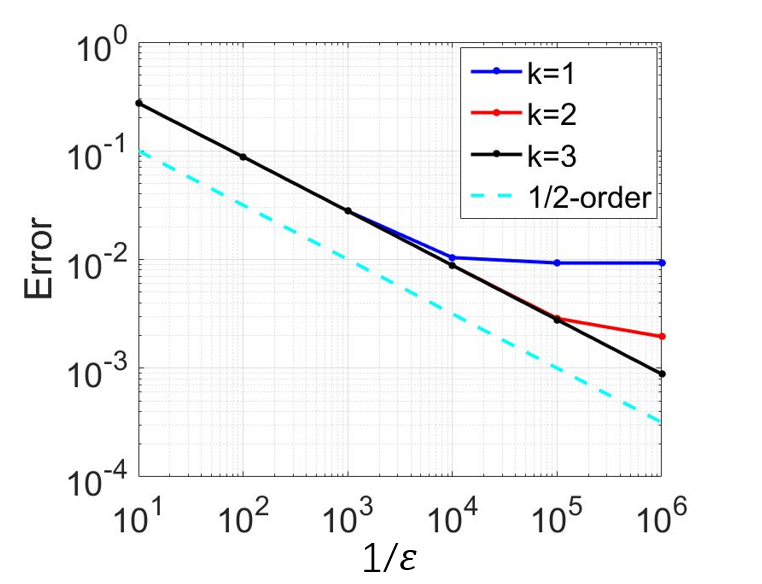
see Figure 1. The triangular partition of Ω\Omega is fixed with meshsize h=0.0295h=0.0295. The numerical errors for different kk and ε\varepsilon are presented in Figure 2. For fixed small ε\varepsilon, the numerical errors, dominated by the errors arising from discontinuous Galerkin approximation, decay as kk increase. On the other hand, for fixed large kk, the numerical errors are dominated by the term εs\varepsilon^{s} with s=α2​(α+2)s=\frac{\alpha}{2(\alpha+2)} given in (2.15). The results demonstrate the convergence of numerical errors with respect to ε\varepsilon with order nearly O⁡(ε1/2)O(\varepsilon^{1/2}) which corresponds to the exact theoretical rate since |∇uσ||\nabla u_{\sigma}| does not vanish here (Theorem 2.2). The numerical reconstructions for k=3k=3 are shown in Figure 3 with the corresponding relative L2L^{2}-errors for different choices of ε\varepsilon.

Refer to caption Refer to caption
(a) uσu_{\sigma} (b) γ\gamma
Figure 1: Example 1. The exact uσu_{\sigma} (a) and γ\gamma (b).
Refer to caption
Figure 2: Example 1. Numerical errors of the reconstruction for different kk and ε\varepsilon.
Refer to caption Refer to caption Refer to caption
(a) ε=10−1\varepsilon=10^{-1} (b) ε=10−3\varepsilon=10^{-3} (c) ε=10−5\varepsilon=10^{-5}
Figure 3: Example 1. The reconstruction of γ\gamma for different ε\varepsilon with relative errors RError=4.31×10−24.31\times 10^{-2}, 4.45×10−44.45\times 10^{-4} and 4.46×10−64.46\times 10^{-6} in (a,b,c), respectively.

Example 2. In this example, we consider the reconstruction of the conductivity function given by

σ⁡(x1,x2)=q⁡(3​(2​x1−1),3​(2​x2−1)),\displaystyle\sigma(x_{1},x_{2})=q(3(2x_{1}-1),3(2x_{2}-1)),

where

q⁡(x1,x2)\displaystyle q(x_{1},x_{2}) =\displaystyle= 1+0.3​(1−x1)2​e−x12−(x2+1)2−(15​x1−x13−x25)​e−x12−x22\displaystyle 1+0.3(1-x_{1})^{2}e^{-x_{1}^{2}-(x_{2}+1)^{2}}-(\frac{1}{5}x_{1}-x_{1}^{3}-x_{2}^{5})e^{-x_{1}^{2}-x_{2}^{2}}
−130​e−(x1+1)2−x22,\displaystyle-\frac{1}{30}e^{-(x_{1}+1)^{2}-x_{2}^{2}},

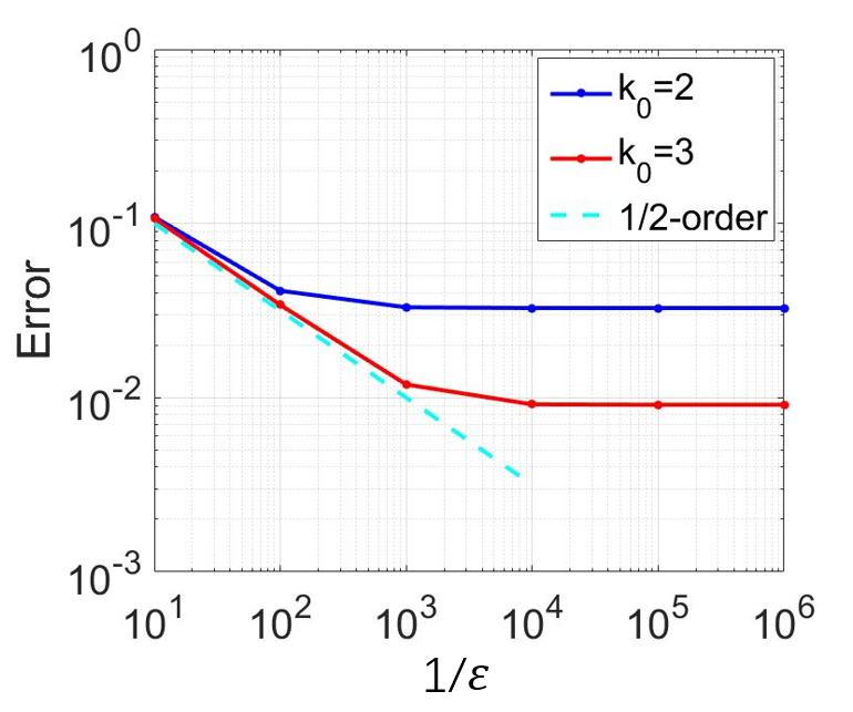
see Figure 4. Set g=ex1+x2−(e2−1)/2g=e^{x_{1}+x_{2}}-(e^{2}-1)/2 on Γ\Gamma satisfying ∫Γg​𝑑x=0\int_{\Gamma}g\,dx=0. The solution uσu_{\sigma} and |∇uσ||\nabla u_{\sigma}| are presented in Figure 5. For simplicity, let the exact measurement data be the polynomial coefficients of the discontinuous Galerkin approximation of uσu_{\sigma} in Pk0​(Th),k0≥2P^{k_{0}}(T_{h}),k_{0}\geq 2. In other words, in each triangular element, we have at least (k0+1)​(k0+2)2\frac{(k_{0}+1)(k_{0}+2)}{2} measurement points to produce the measurement data. The triangular partition of Ω\Omega is fixed with meshsize h=0.0295h=0.0295. Choosing k0=1k_{0}=1 will result into poor reconstruction since in this case Δ​uσ=0\Delta u_{\sigma}=0 in each element. We choose the parameter k=k0k=k_{0}. The reconstruction results are presented in Figures 6 and 7 and the corresponding numerical errors are displayed in Figure 8. The accuracy limitation at a level of approximately 10−210^{-2} corresponds to the number of measurement points and the approximations of ∇uσ\nabla u_{\sigma} and Δ​uσ\Delta u_{\sigma}.

Refer to caption
Figure 4: Example 2. The exact γ\gamma.
Refer to caption Refer to caption
(a) uσu_{\sigma} (c) |∇uσ||\nabla u_{\sigma}|
Figure 5: Example 2. Exact data uσu_{\sigma} and |∇uσ||\nabla u_{\sigma}|.
Refer to caption Refer to caption Refer to caption
(a) ε=10−1\varepsilon=10^{-1} (b) ε=10−3\varepsilon=10^{-3} (c) ε=10−5\varepsilon=10^{-5}
Figure 6: Example 2. The reconstruction of γ\gamma when k0=2k_{0}=2 for different ε\varepsilon with relative errors RError=1.71×10−21.71\times 10^{-2}, 2.53×10−32.53\times 10^{-3} and 2.50×10−32.50\times 10^{-3} in (a,b,c), respectively.
Refer to caption Refer to caption Refer to caption
(a) ε=10−1\varepsilon=10^{-1} (b) ε=10−3\varepsilon=10^{-3} (c) ε=10−5\varepsilon=10^{-5}
Figure 7: Example 2. The reconstruction of γ\gamma when k0=3k_{0}=3 for different ε\varepsilon with relative errors RError=1.66×10−21.66\times 10^{-2}, 4.04×10−44.04\times 10^{-4} and 3.64×10−43.64\times 10^{-4} in (a,b,c), respectively.
Refer to caption
Figure 8: Example 2. Numerical errors of the reconstruction for different k0k_{0} and ε\varepsilon.

Example 3. Next, we consider the reconstruction of conductivity function discussed in Example 2 from noised data

Uδ=uσ​(1+δ​ξ),\displaystyle U^{\delta}=u_{\sigma}(1+\delta\xi),

where δ\delta is the noise level and ξ\xi is an independent and uniformly distributed random variable generated between -1 and 1. Figure 9 displays the perturbated data UδU^{\delta} and ∇Uδ\nabla U^{\delta} with δ=10%\delta=10\% random noise. In addition, less point measurements are taken under a triangular partition of Ω\Omega with meshsize h=0.0589h=0.0589 and we choose k0=2k_{0}=2. The reconstruction results from noised measurement with level δ=5%\delta=5\% are shown in Figures 10 and 11 which demonstrate the high efficiency and robustness of the proposed inversion algorithm. Figure 12 displays the convergence of numerical errors with respect to δ+ε\delta+\varepsilon.

Refer to caption Refer to caption
(a) UδU^{\delta} (c) |∇Uδ||\nabla U^{\delta}|
Figure 9: Example 3. Perturbated data data UδU^{\delta} and |∇Uδ||\nabla U^{\delta}| with 10%10\% random noise.
Refer to caption Refer to caption Refer to caption
(a) ε=0.1\varepsilon=0.1 (b) ε=0.06\varepsilon=0.06 (c) ε=0.01\varepsilon=0.01
Figure 10: Example 3. The reconstruction of γ\gamma from noised measurements when k0=2k_{0}=2, δ=5%\delta=5\% for different ε\varepsilon with relative errors RError=2.24×10−22.24\times 10^{-2}, 1.71×10−21.71\times 10^{-2} and 1.22×10−21.22\times 10^{-2} in (a,b,c), respectively.
Refer to caption Refer to caption Refer to caption
(a) ε=0.1\varepsilon=0.1 (b) ε=0.06\varepsilon=0.06 (c) ε=0.01\varepsilon=0.01
Figure 11: Example 3. The reconstruction of γ\gamma from noised measurements when k0=2k_{0}=2, δ=10%\delta=10\% for different ε\varepsilon with relative errors RError=2.46×10−22.46\times 10^{-2}, 2.04×10−22.04\times 10^{-2} and 1.74×10−21.74\times 10^{-2} in (a,b,c), respectively.
Refer to caption
Figure 12: Example 3. Numerical errors of the reconstruction for different noise level δ\delta and ε\varepsilon.

Example 4. Finally, we consider the reconstruction of a piecewise constant conductivity, see Figure 13. For simplicity, the exact uσu_{\sigma} in Ω\Omega is set to be

uσ=cos⁡(x1−0.5)​ex2.\displaystyle u_{\sigma}=\cos(x_{1}-0.5)e^{x_{2}}.

The reconstruction from perturbated point measurement with 10%10\% random noise presented in Figure 14 shows the efficiency of the proposed method.

Refer to caption
Figure 13: Example 4. The exact γ\gamma.
Refer to caption Refer to caption Refer to caption
(a) ε=0.1\varepsilon=0.1 (b) ε=0.06\varepsilon=0.06 (c) ε=0.01\varepsilon=0.01
Figure 14: Example 4. The reconstruction of γ\gamma from noised measurements when k0=2k_{0}=2, δ=10%\delta=10\% for different ε\varepsilon with relative errors RError=3.79×10−23.79\times 10^{-2}, 2.88×10−22.88\times 10^{-2} and 2.29×10−22.29\times 10^{-2} in (a,b,c), respectively.

Appendix A

Lemma A.1.

(Traces and integration by parts [12, 19] )
The trace operator

γ:C0​(Ω¯)∋v↦γ⁡(v):=v|∂Ω∈L2​(|β⋅ν|,∂Ω)\displaystyle\gamma:C^{0}(\overline{\Omega})\ni v\mapsto\gamma(v):=v|_{\partial\Omega}\in L^{2}(|\beta\cdot\nu|,\partial\Omega)

extends continuously to VV, meaning that there is CγC_{\gamma} such that, for all v∈Vv\in V,

‖γ⁡(v)‖L2​(|β⋅n|,∂Ω)≤Cγ​‖v‖V.\displaystyle\|\gamma(v)\|_{L^{2}(|\beta\cdot n|,\partial\Omega)}\leq C_{\gamma}\|v\|_{V}.

Moreover, the following integration by parts formula holds true: For all v,w∈Vv,w\in V,

∫Ω[(β⋅∇v)​w+(β⋅∇w)​v+(∇⋅β)​v​w]​𝑑x=∫∂Ω(β⋅ν)​γ​(v)​γ​(w)​𝑑s.\displaystyle\int_{\Omega}\left[(\beta\cdot\nabla v)w+(\beta\cdot\nabla w)v+(\nabla\cdot\beta)vw\right]dx=\int_{\partial\Omega}(\beta\cdot\nu)\gamma(v)\gamma(w)ds.
Theorem A.2.

(The Banach-Nečas-Babuška Theorem [20])
Let XX be a Banach space and let YY be a reflexive Banach space. Let a∈ℒ⁡(X×Y,ℝ)a\in\mathcal{L}(X\times Y,\mathbb{R}) and let f∈Y′f\in Y^{\prime}. Then the problem:

Find​u∈X​such that​a​(u,w)=⟨f,w⟩Y′,Y​for all​w∈Y.\displaystyle\mbox{Find}\;\;u\in X\;\;\mbox{such that}\;\;a(u,w)=\langle f,w\rangle_{Y^{\prime},Y}\;\;\mbox{for all}\;\;w\in Y.

is well-posed if and only if:
(i). There is Cs​t​a>0C_{sta}>0 such that

Cs​t​a​‖v‖X≤sup0≠w∈Ya⁡(v,w)‖w‖Y,∀v∈X.\displaystyle C_{sta}\|v\|_{X}\leq\sup_{0\neq w\in Y}\frac{a(v,w)}{\|w\|_{Y}},\quad\forall v\in X. (A.1)

(ii). For all w∈Xw\in X,

(∀v∈X,a(v,w)=0)⟹(v=0).\displaystyle(\forall v\in X,a(v,w)=0)\Longrightarrow(v=0). (A.2)
Lemma 2.3.

Further c>0c>0 is a constant that only depends on gg, σ\sigma, Ω\Omega, and eventually on η\eta. Since uσu_{\sigma} is a solution to the system (1.1), |∇uσ||\nabla u_{\sigma}| is a Mukenhoupt weight. Indeed there exists a contant p>1p>1 depending only on gg, σ\sigma and Ω\Omega such that the following inequality (Theorem 1.1 in [15])

(1|Br​(x)|​∫Br​(x)|∇uσ|​𝑑y)​(1|Br​(x)|​∫Br​(x)|∇uσ|−1p−1​𝑑y)p−1≤c,\displaystyle\left(\frac{1}{|B_{r}(x)|}\int_{B_{r}(x)}|\nabla u_{\sigma}|dy\right)\left(\frac{1}{|B_{r}(x)|}\int_{B_{r}(x)}|\nabla u_{\sigma}|^{-\frac{1}{p-1}}dy\right)^{p-1}\leq c, (A.3)

holds for all r∈(0,η)r\in(0,\eta), and x∈Ωηx\in\Omega_{\eta}.

The following behavior is related to the unique continuation properties of solutions to elliptic equations in a divergence form (Corollary 3.1 in [10]).

c​rβ≤1|Br​(x)|​∫Br|∇uσ|​𝑑y,\displaystyle cr^{\beta}\leq\frac{1}{|B_{r}(x)|}\int_{B_{r}}|\nabla u_{\sigma}|dy, (A.4)

where β≥0\beta\geq 0 is a constant that only depends on gg, σ\sigma and Ω\Omega. The constants β\beta and p>1p>1 are related to the vanishing order of ∇uσ\nabla u_{\sigma} in Ωη\Omega_{\eta}. Combining inequalities (A.3) and (A.4), we obtain

∫Br​(x)|∇uσ|−1p−1​𝑑y≤c​r−β+np−1,\displaystyle\int_{B_{r}(x)}|\nabla u_{\sigma}|^{-\frac{1}{p-1}}dy\leq cr^{\frac{-\beta+n}{p-1}}, (A.5)

for all r∈(0,η)r\in(0,\eta), and x∈Ωηx\in\Omega_{\eta}.

Fix now r=η2r=\frac{\eta}{2}. There exist N∈ℕN\in\mathbb{N} and xj, 1≤j≤N,x_{j},\,1\leq j\leq N, that only depend on η\eta and Ω\Omega such that Ωη⊂∪j=1NBr(xj)\Omega_{\eta}\subset\cup_{j=1}^{N}B_{r}(x_{j}). Let (ϕj)1≤j≤N(\phi_{j})_{1\leq j\leq N} be a partition of unity subordinate to the covering ∪j=1NBr(xj)\cup_{j=1}^{N}B_{r}(x_{j}). We deduce from (A.5), the following estimates

∫Ωη|∇uσ|−1p−1​𝑑y\displaystyle\int_{\Omega_{\eta}}|\nabla u_{\sigma}|^{-\frac{1}{p-1}}dy =\displaystyle= ∑j=1N∫Ωη|∇uσ|−1p−1​ϕj​𝑑y\displaystyle\sum_{j=1}^{N}\int_{\Omega_{\eta}}|\nabla u_{\sigma}|^{-\frac{1}{p-1}}\phi_{j}dy (A.6)
≤\displaystyle\leq ∑j=1N‖ϕj‖L∞​(Ωη)​∫Br​(xj)|∇uσ|−1p−1​𝑑y\displaystyle\sum_{j=1}^{N}\|\phi_{j}\|_{L^{\infty}(\Omega_{\eta})}\int_{B_{r}(x_{j})}|\nabla u_{\sigma}|^{-\frac{1}{p-1}}dy
≤\displaystyle\leq c.\displaystyle c.

Recall Ωη∖Ωηt¯={x∈Ωη:|∇uσ|<t}\Omega_{\eta}\setminus\overline{\Omega^{t}_{\eta}}=\left\{x\in\Omega_{\eta}:\,|\nabla u_{\sigma}|<t\right\}. Assuming that Ωη∖Ωηt¯\Omega_{\eta}\setminus\overline{\Omega^{t}_{\eta}} is not empty, we infer from (A.6) the following inequality

t−1p−1​|Ωη∖Ωηt¯|≤∫Ωη∖Ωηt¯|∇uσ|−1p−1​𝑑y≤∫Ωη|∇uσ|−1p−1​𝑑y≤c,\displaystyle t^{-\frac{1}{p-1}}|\Omega_{\eta}\setminus\overline{\Omega^{t}_{\eta}}|\leq\int_{\Omega_{\eta}\setminus\overline{\Omega^{t}_{\eta}}}|\nabla u_{\sigma}|^{-\frac{1}{p-1}}dy\leq\int_{\Omega_{\eta}}|\nabla u_{\sigma}|^{-\frac{1}{p-1}}dy\leq c,

which in turn leads to

0≤|Ωη∖Ωηt¯|≤c​tα,\displaystyle 0\leq|\Omega_{\eta}\setminus\overline{\Omega^{t}_{\eta}}|\leq ct^{\alpha},

with α:=1p−1>0\alpha:=\frac{1}{p-1}>0. ∎

References

  • [1] R. A. Adams and J. F. Fournier, Sobolev Spaces (Second ed.), Academic Press, 2003.
  • [2] G. Alessandrini, An identification problem for an elliptic equation in two variables, Annalidi Matematica Pura ed Applicata, 145 (1986), pp. 265–295.
  • [3] H. Ammari, J. Garnier, H. Kang, L. H. Nguyen, and L. Seppecher, Multi-Wave Medical Imaging: Mathematical Modelling & Imaging Reconstruction, World Scientific, London, 2017.
  • [4] N. Antonić and K. Burazin, Intrinsic boundary conditions for friedrichs systems, Communications in Partial Differential Equations, 35(9) (2010), pp. 1690–1715.
  • [5] G. Bal and G. Uhlmann, Reconstruction of coefficients in scalar second-order elliptic equations from knowledge of their solutions, Comm. Pure Appl. Math., 66(10) (2013), pp. 1629–1652.
  • [6] P. Binev, A. Cohen, W. Dahmen, R. DeVore, G. Petrova, and P. Wojtaszczyk, Convergence rates for greedy algorithms in reduced basis methods, SIAM J. Math. Anal., 43(3) (2011), pp. 1457–1472.
  • [7] E. Bonnetier, M. Choulli, and F. Triki, Hölder stability for the qualitative photoacoustic tomography, submitted, (2019).
  • [8] M. Briane, Reconstruction of isotropic conductivities from non smooth electric fields, ESAIM: Math. Model. Numer. Anal., 52(3) (2018), pp. 1173–1193.
  • [9] M. Briane, G. W. Milton, and A. Treibergs, Which electric fields are realizable in conducting materials, ESAIM: Math. Model. Numer. Anal., 48(2) (2014), pp. 307–323.
  • [10] M. Choulli and F. Triki, New stability estimates for the inverse medium problem with internal data, SIAM J. Math. Anal, 47(3) (2015), pp. 1778–1799.
  • [11] M. Choulli and E. Zuazua, Lipschitz dependence of the coefficients on the resolvent and greedy approximation for scalar elliptic problems, C. R. Math. Acad. Sci. Paris, Ser I, 354 (2016), pp. 1174–1187.
  • [12] A. Ern, J.-L. Guermond, and G. Caplain, An intrinsic criterion for the bijectivity of hilbert operators related to friedrichs’ systems, Communications in Partial Differential Equations, 32 (2007), pp. 317–341.
  • [13] G. Fichera, Sulle equazioni differenziali lineari ellittico-paraboliche del secondo ordine, Atti Accad. Naz. Lincei Mem. Cl. Sci. Fis. Mat. Nat. Sez. I, 5(8) (1956), pp. 1–30.
  • [14] K. O. Friedrichs, Symmetric positive linear differential equations, Comm. Pure Appl. Math., 11 (1958), pp. 333–418.
  • [15] N. Garofalo and F.-H. Lin, Monotonicity properties of variational integrals, apa_{p} weights and unique continuation, Indiana Univ. Math. J., 35(2) (1986), pp. 245–268.
  • [16] J. J. Kohn and L. Nirenberg, Degenerate elliptic-parabolic equations of second order, Comm. Pure Appl. Math., 20 (1967), pp. 797–872.
  • [17] O. A. Oleinik and E. V. Radkevic, Second Order Equations with Nonnegative Characteristic Form, Plenum Press, New York, 1973.
  • [18] P. Pavel and J. Sokolowski, Compressible Navier-Stokes equations: theory and shape optimization, Birkhäuser Basel, 2012.
  • [19] D. A. D. Pietro and A. Ern, Mathematical Aspects of Discontinuous Galerkin Methods, Mathématiques & Applications, Springer-Verlag, 2012.
  • [20] B. Rivière, Discontinuous Galerkin Methods for Solving Elliptic and Parabolic Equations: Theory and Implementation, SIAM, 2008.