Two-moment scheme for general-relativistic radiation hydrodynamics: a systematic description and new applications2020
Abstract
We provide a systematic description of the steps necessary – and of the potential pitfalls to be encountered – when implementing a two-moment scheme within an Implicit-Explicit (IMEX) scheme to include radiative-transfer contributions in numerical simulations of general-relativistic (magneto-)hydrodynamics. We make use of the M1 closure, which provides an exact solution for the optically thin and thick limit, and an interpolation between these limits. Special attention is paid to the efficient solution of the emerging set of implicit conservation equations. In particular, we present an efficient method for solving these equations via the inversion of a -matrix within an IMEX scheme. While this method relies on a few approximations, it offers a very good compromise between accuracy and computational efficiency. After a large number of tests in special relativity, we couple our new radiation code, FRAC, with the general-relativistic magnetohydrodynamics code BHAC to investigate the radiative Michel solution, namely, the problem of spherical accretion onto a black hole in the presence of a radiative field. By performing the most extensive exploration of the parameter space for this problem, we find that the accretion’s efficiency can be expressed in terms of physical quantities such as temperature, , luminosity, , and black-hole mass, , via the expression , where and are the Eddington luminosity and accretion rate, respectively. Finally, we also consider the accretion problem away from spherical symmetry, finding that the solution is stable under perturbations in the radiation field.
Keywords:
radiation: dynamics – radiative transfer – MHD – methods: numerical – accretion, accretion discs – black hole physics – gravitation1 Introduction
The study of high-energy astrophysical phenomena plays an increasingly important role in understanding the fundamental laws of the universe. One reason for this was the beginning of the multimessenger era, which was ushered in by the first detection of gravitational waves of a binary neutron star system by the LIGO/VIRGO collaboration (The LIGO Scientific Collaboration & The Virgo Collaboration 2017) and its electromagnetic counterpart (The LIGO Scientific Collaboration et al. 2017; Abbott et al. 2017). This event, GW170817, provided a wealth of information not just on the nature of gravity, but also on the properties of matter under extreme conditions (see Margalit & Metzger 2017; Bauswein et al. 2017; Rezzolla et al. 2018; Ruiz et al. 2018; Annala et al. 2018; Radice et al. 2018; Most et al. 2018; Coughlin et al. 2018; Burgio et al. 2018; Tews et al. 2018; Shibata et al. 2019; Koeppel et al. 2019, for an incomplete list). Another milestone for high-energy astrophysics were the millimetre-wavelength observations by the Event Horizon Telescope (EHT) collaboration, which delivered the first spatially resolved image of a black-hole shadow in the center of the galaxy M87 (Event Horizon Telescope Collaboration et al. 2019a; Event Horizon Telescope Collaboration et al. 2019b; Event Horizon Telescope Collaboration et al. 2019c). This image shows an asymmetric emission ring around the central black hole, which can be explained by the model of a Kerr black hole within the context of general relativity.
Both of these recent milestones have in common that the understanding of these observations was aided by numerical simulations, either of binary neutron stars (see, e.g., Baiotti & Rezzolla 2017; Paschalidis 2017, for reviews) or the accretion onto black holes (see, e.g., Abramowicz & Fragile 2013, for a review). These systems are nowadays simulated by solving numerically the equations of general-relativistic magnetohydrodynamics (GRMHD). However, as the realism of these simulations increases, it becomes necessary to include the coupling between the fluid describing the neutron star or the accretion disk with radiation in the form of photons or neutrinos, resulting in what is called general-relativistic radiative-transfer MHD (GRRTMHD). In standard simulations of geometrically thick, optically thin accretion disks, this coupling is less important and it is therefore adequate to neglect the backreaction onto the fluid of the radiation, which can instead be handled independently and in a post-processing stage (Mizuno et al. 2018; Event Horizon Telescope Collaboration et al. 2019b; Davelaar et al. 2019). Although neglecting the interaction between fluid and the radiation field is a good approximation for a low-luminosity active galactic nuclei (LLAGNs) such as Sgr A*, the inclusion of radiative cooling has been recently considered to produce self-consistent models of another LLAGN such as M87 (Mościbrodzka et al. 2011; Dibi et al. 2012). Detailed simulations of this source including radiation interaction were carried out recently by Chael et al. 2019. On the other hand, in systems of compact objects with high accretion rates, i.e., close to or above their Eddington limit, the disk cools efficiently via the production of photons that are then radiated to infinity. In such radiation-dominated accretion flows, the dynamical interaction between radiation and fluid becomes non-negligible (see McKinney et al. 2014, and reference therein). Also for binary neutron-star simulations, and especially during the post-merger phase, the dynamical evolution of radiation in the form of neutrinos and the full coupling to the fluid is necessary. Indeed, after the merger of two neutron stars, the composition and amount of the ejected material can be significantly altered due to interactions of the fluid with neutrinos that are produced within the hot merger remnant. The properties of this material are directly connected to the resulting kilonova, which results from the radioactive decay of elements produced via r-process in the ejected material (Rosswog et al. 2014; Dietrich & Ujevic 2017; Siegel & Ciolfi 2016; Bovard et al. 2017; Perego et al. 2017; Fujibayashi et al. 2018; Siegel & Metzger 2017; Fernández et al. 2019; Most et al. 2019b). It is thus necessary to solve the equations of radiative transport in conjunction with those describing the dynamics of the fluid.
The equation describing the evolution of the radiation field is given by the Boltzmann equation (Rezzolla & Zanotti 2013, see, e.g., ), which is seven-dimensional (7D), since it has to evolve in time (one dimension) variables defined both in the spatial space (three dimensions) and in the momentum space (three dimensions). In contrast to the four-dimensional (4D) equations of GRMHD, the numerical cost for solving the full Boltzmann equation is prohibitive. Therefore, many approximate schemes have been developed over the years. The most basic scheme is the so-called “leakage-scheme”, which only considers cooling of the fluid via the emission of the radiation (Ruffert et al. 1996; Rosswog & Liebendörfer 2003; Galeazzi et al. 2013; Perego et al. 2014), while heating through absorption is neglected. A more accurate, yet still approximate and feasible, approach is provided by the moment scheme. Within this scheme, which is based on Thorne’s moment formalism (Thorne 1981) – and first implemented within general relativity by Rezzolla & Miller 1994; Shibata et al. 2011; Cardall et al. 2013 – only the first few moments of the radiation distribution function are evolved. Within this formalism, the lowest-order approximation is then represented by the evolution of only the zeroth moment, and is often referred to as the flux-limited diffusion limit [Pomraning 1981; Levermore & Pomraning 1981; see also Rahman et al. 2019 for an implementation of this scheme]. This approximation is particularly suited for spherically symmetric problems, because it does not provide any information about the direction of the radiation fluxes. This can be achieved, however, when evolving also the first moment (momentum density) of the distribution function in what is also called the “M1 scheme”. While this choice introduces three more variables to be evolved in 3D (the energy flux is a three-vector), the M1 scheme offers the best compromise between accuracy and feasibility and has widely been used in the context of black-hole accretion (Zanotti et al. 2011; Fragile et al. 2012; Roedig et al. 2012; Sa̧dowski et al. 2013; Fragile et al. 2014; McKinney et al. 2014), core-collapse supernovae (O’Connor 2015; Just et al. 2015; Kuroda et al. 2016), black-hole–neutron-star mergers (Foucart et al. 2015; Foucart et al. 2016b) and binary neutron stars (Foucart et al. 2016a; Sekiguchi et al. 2016). Because of the related very high computational costs, more accurate methods – such as the Monte-Carlo scheme (Foucart 2018; Miller et al. 2019b) – have so far been considered only in the post-processing of a binary neutron-star simulation (Foucart et al. 2018) or during the post-merger phase with a fixed spacetime (Miller et al. 2019a).
We here present a detailed description of our implementation of the M1 scheme within the stand-alone Frankfurt Radiation Code, FRAC, that can easily be coupled to already existing GRMHD codes, either in fixed spacetimes or in arbitrary and dynamically evolving spacetimes. Several different implementations of the M1 scheme can be found in the literature and to guide the reader in this rather ample literature we note that the biggest differences among the various codes can be restricted to three main aspects, which will be discussed in detail throughout this work:
- •
the type of closure that determines which limit (optically thin and/or thick) can be treated (see Sec. 2.3 for details).
- •
the treatment of the radiative-transfer equations in the stiff limit. Here, we make use of an IMEX scheme (Pareschi & Russo 2005) in order to assure numerical stability also in the optically thick regime (see Sec. 2.5 for details). Keeping in mind the high computational cost for binary neutron-star simulations, we present an efficient way to solve the implicit equations of the IMEX scheme, which represents a good compromise between accuracy and computational cost.
- •
the inclusion of a dependence on the frequency of the radiation. The evolved moments, in fact, depend not just on space and time, but also on the frequency of the photon/neutrino (see Sec. 2.2). The inclusion of this additional dependency drastically increases the computational cost and has been so far considered only in few cases, as, e.g., in the one-dimensional code of O’Connor 2015. For simplicity, no frequency dependence is considered here.
Besides the obvious presentation of a large set of tests in special relativity, there are two important aspects in which our work here differs from those presented so far in the literature. First, we provide a rather detailed description of the numerical issues and problems that had to be faced and solved when implementing the M1 scheme in a generic general-relativistic MHD context, both in stationary and analytic spacetime, but also within codes employed to simulate binary neutron-star mergers. We hope that, in this way, many of the unexpected pitfalls we have encountered and that were not documented before, can be easily avoided by those wanting to replicate our results. Second, we consider as a rather stringent test of our approach in a curved spacetime a problem that actually has an astrophysical application, deriving an expression that could be of interest in astronomy.
More specifically, we consider the problem of a spherically symmetric accretion flow onto a black hole. While closed-form solutions are present in the absence of radiation (Bondi 1952; Michel 1972), this scenario can only be solved within a general-relativistic radiative-transfer (GRRT) context when the ordinary fluid is coupled non-trivially with a radiation fluid11 1 Magnetic fields could in principle be introduced, but would imply a rather artificial scenario involving a monopolar magnetic field and an arbitrary strength. Indeed, this is a classical GRRT problem, which has been studied in the past (Vitello 1978; Nobili et al. 1991) and more recently (Fragile et al. 2012; Roedig et al. 2012; Sa̧dowski et al. 2013; Fragile et al. 2014; McKinney et al. 2014). Here, we explore the largest space of parameters characterising this problem and obtain in this way a simple and useful relation between the accretion efficiency and the black-hole’s bolometric luminosity and mass. Such an expression allows one, therefore, to simply relate observable quantities, such as the luminosity and the temperature of the infalling fluid, to the mass of the black hole. Finally, we also simulate this problem away from spherical symmetry via introducing perturbations in the in the accreting flow and hence in the radiation field. Our simulations show that the accretion flow is stable and returns to its equilibrium after radiating to infinity the excess energy introduced by the perturbation. This result complements the interesting investigation of the Michel solution recently performed by Tejeda et al. 2020; Waters et al. 2020 and which indicates that the dynamics of this scenario is richer than what expected so far.
The paper is organised as follows: in Sec. 2 we list the equations of the truncated moment formalism and discuss the details of our implementation, including the closure (Sec. 2.3), the computation of the fluxes (Sec. 2.4) and the IMEX scheme (Sec. 2.5). We then show the validity of our implementation with a number of standard-tests in Sec. 3. After verifying the correct coupling of FRAC with the “Black Hole Accretion Code” (BHAC) (Porth et al. 2017; Olivares et al. 2019) in Sec. 3.6, we finally apply the coupled code to the problem of spherically symmetric accretion onto a black hole in Sec. 4.2. In Sec. 4.3 we present the solution of this problem when deviating from spherical symmetry and finally conclude and summarizes in Sec. 5.
Hereafter, Latin indices run from to , while Greek indices run from to , and the signature of the metric tensor is assumed to be . We also use the Einstein summation convention over repeated indices and geometrised units in which the speed of light and the gravitational constant . Appendix A is dedicated to the tedious but error-prone procedure needed to transform from these units over to physical CGS units.
2 Two-moment scheme for radiative transfer
Before describing the equations of general-relativistic radiative transfer (GRRT), we briefly summarizes the equations of ideal GRMHD that describe the motion of the ordinary fluid (in the absence of radiation) and that will need to be coupled to those describing the evolution of the radiation fluid (see Sec. 2.6 for details on this coupling).
2.1 General-relativistic MHD
We recall that the ordinary fluid is described by the conservation equations of mass and energy-momentum and by Faraday’s induction equation (with zero resistivity), i.e.,
| (1) | ||||
| (2) | ||||
| (3) |
with being the fluid rest-mass density, its four-velocity, the fluid energy-momentum tensor, which includes contributions from the matter and the electromagnetic fields, and the dual Faraday tensor .
In modern numerical codes, Eqs. (1)–(3) are solved numerically after being cast in a conservative formulation in order to assure numerical stability and convergence to the correct solution in the presence of shocks (Rezzolla & Zanotti 2013). Overall, they have the schematic form
| (4) | |||
| (5) | |||
| (6) | |||
| (7) |
where we recall that is the determinant of the spatial three-metric, is the conserved rest-mass density, is the rescaled total fluid energy density, the components of the covariant three-momentum, and the components of the magnetic field, all in the Eulerian frame [see, e.g., , Porth et al. 2017 for details and the numerical methods normally employed to solve such equations].
In the presence of radiation, Eq. (2) has to be modified since now is no longer conserved, but rather the total energy-momentum tensor is conserved, i.e., , where is the energy-momentum tensor of the radiation fluid. It follows that
| (8) |
so that can be regarded as an external “four-force”.
While we will provide an explicit expression for and in the next section, together with the details on how to couple fluid and radiation in a numerical code in Sec. 2.6, we here only mention that when cast in a conservative formulation, the evolution equations (1) and (3) [or, equivalently, Eqs. (4), (7)] remain unaltered (the radiation fluid does not alter the fluid’s particle number and is not charged, thus does not backreact on the background magnetic field), while (2) will need to be suitably modified to account for the radiation contributions to the total energy density and momentum.
Next, we describe our treatment of the radiation via a two-moment scheme, which is widely used in radiation-hydrodynamics codes (Roedig et al. 2012; Sa̧dowski et al. 2013; McKinney et al. 2014; O’Connor 2015; Foucart et al. 2015; Melon Fuksman & Mignone 2019, see, e.g., ). In our implementation, we mostly follow Foucart et al. 2015, which itself is based on the work of Shibata et al. 2011 and Cardall et al. 2013.
2.2 General-relativistic radiative transfer
Radiation in form of photons or neutrinos is described by their distribution function , which depends on the spatial coordinates and the particles momentum (see, e.g., Rezzolla & Zanotti 2013, and references therein). This distribution function changes in time according to the Boltzmann equation
| (9) |
where are the Christoffel symbols and the affine parameter of a radiation particle’s trajectory. The right-hand side includes the collisional processes such as emission, absorption and scattering. Because Eq. (9) represents a 7D problem that is, in general, too expensive to solve numerically, we adopt a formalism in which the radiation field is described in terms of moments of the distribution function and expressed in terms of projected, symmetric and trace-free tensors (Thorne 1981). In practice, we then employ an approximation that involves the evolution of the lowest-two moments of the distribution function (Rezzolla & Miller 1994; Shibata et al. 2011). More specifically, within a 3+1 decomposition of spacetime (Alcubierre 2008; Gourgoulhon 2012), one evolves the two moments of the distribution function that are thus defined as
| (10) | ||||
| (11) |
where the integrals are taken in a frame comoving with the fluid (i.e., the “fluid frame”), (not to be confused with a tensor index) is the radiation frequency and is the solid angle on a unit sphere in momentum space and a unit normal four-vector orthogonal to the fluid four-velocity , i.e., .
In practice, the quantities and represent the frequency-dependent (hence the index) definitions of the radiation energy density and of the radiation momentum density, respectively. For simplicity, and to reduce computational costs, we here limit ourselves to frequency-integrated moments, i.e.,
| (12) | ||||
| (13) |
thus to what is commonly referred to as "grey" approximation. Note that a frequency-dependent scheme would require a discretization of the final evolution equations in and thus increase the numerical cost by a factor of , where is the number of bins chosen for this discretization. In addition, we define the second moment as
| (14) |
which represents the stress tensor of the radiation fluid.
Using these moments, it is possible to write the energy-momentum tensor of the radiation as
| (15) |
This tensor can also be written in the Eulerian frame as
| (16) |
where is a timelike unit four-vector normal to a hypersurface when considering the -decomposition of spacetime. The quantities , and are respectively: the radiation energy density, the radiation momentum density and the radiation pressure tensor, all evaluated in in the Eulerian frame. Using the split of the fluid four-velocity as , where is the Lorentz factor and the spatial four-velocity of the fluid in the Eulerian frame, these quantities can be obtained from their counterparts in the fluid frame via
| (17) | ||||
| (18) | ||||
| (19) |
where is the four-metric. Vice-versa, the fluid-frame quantities can be obtained from the Eulerian ones via
| (20) | ||||
| (21) | ||||
| (22) |
where is the projection tensor orthogonal to the fluid four-velocity, i.e., . From these equations it then follows that for any fluid with , the following relations hold: , and . We also note that and are purely spatial by construction, i.e., .
The evolution equations for and in conservative form read
| (23) | ||||
| (24) |
The right-hand sides of the Eqs. (23)–(24) include – in addition to the “geometric source terms” such as the lapse , the shift , the three-metric and its determinant , and the extrinsic curvature – the “collisional source terms”
| (25) |
where is written in terms of the fluid-frame quantities as
| (26) |
Here, is the frequency-integrated emissivity, the frequency-averaged absorption opacity, and is the total opacity, with the frequency-averaged scattering opacity. Formally, the definition of these coefficients follows directly from integrating the Boltzmann equation over and the corresponding expressions are therefore
| (27) | ||||
| (28) | ||||
| (29) |
These quantities essentially embody the coupling of the radiation fluid with the matter fluid and are determined by the underlying microphysics, i.e., the constituents of the radiation fluid (neutrinos or photons) and which interactions and reactions are taken into account. We detail our choices for these parameters in Sec. 4.2.
2.3 Closure
As it is common in moment-expansion approaches, given an expansion of the distribution function at order , the first evolution equations involve the first moments. Hence, when actually calculating a solution, it is necessary to truncate the expansion and introduce a “closure relation”, namely, the -th equation which specifies the value of the highest moment used in terms of lower ones. This closure relation needs to be derived on the basis of physical considerations and may differ from problem to problem (Thorne 1981; Rezzolla & Miller 1994). In practice, what is needed in our two-moment scheme is an explicit expression for the radiation pressure tensor in terms of lower-order moments, i.e., and . Since it is possible to obtain explicit expressions for in the optically thin and optically thick (or “diffusion”) limits, , we express the closure relation as
| (30) |
where is the so-called closure-function and is the variable Eddington-factor and is a measure of the degree of anisotropy of the radiation fluid (Rezzolla & Miller 1994). A possible definition of is therefore
| (31) |
with the second equality holding because . Note that corresponds to the optically thin limit, while to the optically thick one.
Another possible choice for the Eddington factor [used e.g., in Melon Fuksman & Mignone 2019] is instead
| (32) |
with still representing the two optical limits. We here choose Eq. (31) over Eq. (32), although this means a substantially higher computational cost because of the necessity of a root-finding method for computing , which will be detailed below. Nevertheless, Eq. (31) is the correct choice since only this one is accurate in the optically thick limit (Shibata et al. 2011, see).
For the closure-function , we choose instead the so-called Minerbo closure (also referred to as the maximum-entropy closure) after Minerbo 1978 22 2 This closure is often referred to as the M1 closure. However, this is a misnomer since the whole moment-scheme is usually called M1 scheme independent of the closure implemented., which is given by
| (33) |
We note that there are many other possible choices for the closure function , e.g., the often-used Levermore closure (Levermore 1984) and given by
| (34) |
Hereafter, we will make use of Eq. (33), but refer the interested reader to Murchikova et al. 2017 for a comparison between different closures.
We next calculate the radiation-pressure tensor in the two relevant limits starting with the optically thin one (), recalling that in this case , so that we readily obtain
| (35) |
For the thick limit (), on the other hand, we simply compute in terms of the thick-limit expressions for the quantities in Eq. (19), namely
| (36) | ||||
| (37) | ||||
| (38) |
The difficulty with closing the system of Eqs. (23)–(24) lies in the dependence of the Eddington-factor on and , which, in turn, depend on the unknown pressure tensor . It is therefore necessary to obtain via a root-finding method as follows:
- 1.
- 2.
- 3.
check if the function
(39) is below a threshold value. If so, we have found the correct value for . If not we adjust using a Newton-Raphson method, i.e.,
(40) where the derivative has to be computed via a finite-difference method, and then repeat the cycle. Alternatively one could find the root of via Brent’s method, which we find to be more robust, but also computationally more expensive.
We should note that the choice of closing the system of evolution equations with Eq. (30) is computationally more expensive than using the commonly used closure given by
| (41) |
However, the assumptions behind the validity of the closure (41), i.e., isotropic radiation and , hold only in the optically thick limit. Implementations with this choice of closure can therefore model only those astrophysical scenarios where the optical depth is high (Roedig et al. 2012; Fragile et al. 2012, see, e.g., ). Since we do not wish to restrict to such conditions, our implementation with the choice of Eq. (30) allows to model both the thin and the thick regimes.
2.4 Computation of the fluxes
When coupling FRAC with BHAC (Porth et al. 2017), which solves the equations of GRMHD with finite-volume methods, it is simpler to compute Eqs. (23) and (24) using the same finite-volume approach. To accomplish this, we need, therefore, the interface-averaged “fluxes”. For second-order accuracy as the one employed here, these fluxes are obtained by reconstructing the cell-averaged values of and to the mid-points of the interfaces and then using an approximate Riemann solver. Here, we use the minmod reconstruction and the HLL-Riemann solver (see Rezzolla & Zanotti 2013, for an overview of these numerical methods), reconstructing rather than as this then ensures causality. The characteristic speeds for the Riemann solver depend on whether the fluid is optically thick or thin and the limiting cases are again known exactly and given by (Shibata et al. 2011)
| (42) | ||||
| (43) |
with
| (44) |
where and denotes the direction in which the characteristic speeds are evaluated. The final characteristic speeds are then interpolated between the two regimes in the same manner as for the radiation pressure tensor, i.e.,
| (45) |
The Eddington-factor at the cell interfaces is computed after the reconstruction step, which is necessary since the fluxes depend on . In Eq. (45) we can then simply use the same and do not have to recompute it. We note that, because the computation of via root-finding is the most expensive part of the M1 scheme, we also tried other methods to reduce the computational costs. A more efficient method is simply to interpolate from the surrounding cell-centres to the cell-faces (since the source terms also include , it is necessary to compute in the cell centres anyway). Even more efficient, albeit less accurate, would be to simply use the same value of as computed for the cell-centres also at the cell interfaces. No appreciable difference was found regarding the accuracy between all of these methods, so that we adopted the latter, – which is computationally the least expensive – as the default.
After obtaining the fluxes at the cell interface via use of an approximate Riemann solver, we correct them to obtain the correct asymptotic behavior also in the optically thick limit. As will be discussed in Sec. (2.5), the collisional source terms, i.e., and , become large for high optical depth , leading to an inaccurate solution of the system (23)–(24) on a timescale of , where is the proper distance (see below) between two adjacent grid cells (Jin & Levermore 1996). In essence, this results into an incorrect diffusion rate of the radiation through the fluid. In order to correct for this effect, we apply the same flux corrections in the optically thick limit suggested by O’Connor 2015; Foucart et al. 2015, i.e.,
| (46) |
where is the flux in Eq. (23) in -th direction, is the asymptotic flux [see Eq. (48)], and is the weight function chosen as
| (47) |
with at the cell interface between the -th and -th grid-cell approximated as and the proper distance in -th direction, with the coordinate distance. The correct asymptotic flux in the optically thick limit can be evaluated to be (Thorne 1981)
| (48) |
and has to be computed on the cell interfaces. While is already a good approximation to its value on the interface, the other quantities in the last term of Eq. (48), i.e., , , and , are simply computed as the averages of neighbouring cell-centered values. The total derivative of the energy density in the fluid frame along the -th direction is computed as
| (49) |
The quantities in the first two terms in Eq. (48), on the other hand, are computed from their reconstructed left and right states via the advection speed in -th direction defined as
| (50) |
If is positive for both the left and right states, we choose the left state; on the other hand, if it is negative for both the left and right state, we choose the right state. In all other cases we set all quantities in the first two terms in Eq. (48) to zero
Finally, to also ensure the correct behavior in the optically thick limit for the fluxes of , i.e., for the quantities , we choose to correct these fluxes as done in Audit et al. 2002
| (51) |
i.e., the flux at the cell interface is simply corrected with the average of that flux in adjacent cell-centres weighted by a factor .
2.5 Implicit treatment of stiff source terms
As mentioned above, the opacities and can become very large for optically thick fluids. From Eq. (26) it is evident that, under these conditions, also the collisional source terms on the right-hand side of the evolution equations can become very large, thus posing a major difficulty in solving these equations numerically. In these regimes, the explicit numerical solution of Eqs. (23) and (24) requires a prohibitively small timestep, making them “stiff”. More specifically, the timestep would have to be of order , thus making the numerical evolution unfeasible. The situation is analogous to that of resistive magnetohydrodynamics, where the timestep must decrease with resistivity when employing explicit schemes (see Palenzuela et al. 2009; Dionysopoulou et al. 2013; Alic et al. 2012; Ripperda et al. 2019, for an implementation of similar methods for the case of general-relativistic resistive MHD).
A solution to this limitation comes from the adoption of mixed implicit and explicit methods. In what follows we illustrate the use of an implicit-explicit (IMEX) scheme that treats the advection term and the geometric sources explicitly, while treating implicitly the collisional source term. In such a scheme, a generic state vector 33 3 We here denote with the state vector relative to the radiation variables and , while that of the fluid variables will be explicitly marked with a subscript as . From here on, we also write all state vectors and their corresponding flux and source vectors in boldface. is advanced from timestep to the next timestep via intermediate steps denoted as () and given by (Pareschi & Russo 2005)
| (52) | |||
| (53) |
The intermediate steps are computed from a combination of the explicit terms and the implicit terms , which are weighted by the matrices and , respectively. These matrices are chosen so that the coefficients are zero for in the explicit case and for in the implicit case. An IMEX scheme with such matrices is referred to as the diagonally implicit Runge-Kutta (DIRK) IMEX scheme. The matrix elements and , as well as the weights and , can be expressed conveniently via a Butcher tableau and determine the specific type of the scheme and its order. We here restrict ourselves to a second-order scheme with two explicit and two implicit stages [called SS2(2,2,2) in the notation of Pareschi & Russo 2005]. In such a scheme the intermediate steps can be written as
| (54) | ||||
| (55) | ||||
| (56) |
where . Interestingly, it is possible to rewrite the equations above in a way – which corresponds to the one we have actually implemented – that avoids to store any intermediate explicit term , namely, as
| (57) | ||||
| (58) | ||||
| (59) |
where we have also introduced a more convenient notation by writing and by using curly brackets to highlight the explicit part of the equations. Such a notation helps to see that Eqs. (57) and (58) are of the form
| (60) |
where is some intermediate state including all contributions in the curly braces. Obviously and because of the implicit nature of the scheme, the same state appears both on the left- and on the right-hand side of these equations. This implicit nature of the equations for the intermediate states generalises also to higher-order IMEX schemes.
In general, an equation of the type (60) cannot be solved analytically, which poses the biggest difficulty in using an IMEX scheme and overall for the M1 scheme. In what follows we outline three different strategies for solving these equations and start by detailing how the quantities and are related to the evolution equations (23) and (24).
As already mentioned, includes all explicit terms, i.e.,
while all the implicit terms, i.e.,
| (63) |
For each intermediate timestep , there are three different ways of performing the time update. The first and easiest method, which we refer to as “approximate method” proceeds as follows:
- 1.
compute in Eq. (60) from , and , where .
- 2.
linearise the implicit term as
(64) where the matrix and the column-vector depend on the previous intermediate state (or in the case of the zeroth step), which makes this linearisation only approximately true. Actually and would have to depend on the current state as well, in which case the linearisation would not be possible anymore. This approximation is justified under the assumption that the fluid four-velocity and the pressure tensor do not change much during this intermediate timestep. The derivation of and is detailed below.
- 3.
In practice, this approximate method is the one used by Foucart et al. 2015, although not within an IMEX scheme.
The second method, which is an improvement over the previous one and is normally referred to as the “fixed-point” method, has been implemented by Roedig et al. 2012; Fragile et al. 2014; Melon Fuksman & Mignone 2019, and is also used in the context of resistive MHD by Palenzuela et al. 2009; Dionysopoulou et al. 2013; Alic et al. 2012; Ripperda et al. 2019. In such an approach, after step 3., the fluid four-velocity is updated (see below for how the coupling between radiation and the fluid is done) and from this, as well as from the new values for and the pressure tensor is recomputed. Going back to step 2., this procedure is then iterated until the values of for consecutive iterations are below a given threshold value.
A third and final method, which we refer to as the “root-finding” method, consists in solving Eq. (60) directly via a root-finding procedure employing for example a four-dimensional Newton-Raphson method (McKinney et al. 2014; Sa̧dowski et al. 2013; Melon Fuksman & Mignone 2019; Ripperda et al. 2019). Clearly, the fixed-point and the root-find methods are more complex and computationally expensive, so that we here concentrate on results obtained with the approximate method, postponing a detailed comparison among the three methods to a future work.
Independently of which of the three methods discussed above is actually used, it is necessary to write the collisional sources in terms of the evolved variables and , rather than in their counterparts in the fluid frame and . This can be done by using Eqs. (20) and (21) in order to replace and in Eq. (26). In this way, can then be written as
| (66) |
Note that it is not yet possible to write in the desired form as , which is spoiled by the last term in Eq. (2.5). This will only be possible after contracting with and , respectively, as will be necessary for computing according to Eq. (63). After these contractions, the linearisation of Eq. (63) follows as in Eq. (64) with and now given by
where we have introduced the shorthands
| (71) | ||||
| (72) | ||||
| (73) |
and
| (74) |
As a consistency check, it is possible to verify that
| (75) |
with given by Eq. (26).
2.6 Coupling between radiation and the ordinary fluid
At this point we can finally discuss the coupling between the radiation and the ordinary (matter) fluid. As anticipated at the beginning of Sec. 2, this is essentially done by “adding” to the right-hand-sides of the conservative evolution equations of the fluid [Eqs. (5)–(6)], the components of the source-vector , i.e.,
| (76) | |||
| (77) |
As long as the ordinary fluid dominates, i.e., the fluid variables have values that are much larger than the corresponding radiation variables, it is possible to simply treat these additional source terms explicitly, as done in Roedig et al. 2012. However, especially in regions of high optical depth, these source terms may become much larger than the current value of the fluid variables. In this case, the evolution equations for the ordinary fluid, i.e., Eqs. (76) and (77), become stiff and have to be treated implicitly, exactly as we have already illustrated in the case of the evolution equations for the radiation fluid, i.e., Eqs. (23), (24).
In practice, this is now rather straightforward and simply requires to compute the source term of the fluid
| (78) |
and to add it to the state vector , which is the intermediate state in Eq. (60), but this time for the fluid variables.
Note that within this approach, the term has not been computed up to this point, because Eq. (60) for the radiation is solved via Eq. (65). However, with and , which have already been computed for this purpose, at every substep it is possible to obtain easily via Eq. (64) using the newly computed of the radiation. In this way, Eq. (60) is solved and the collisional source term is automatically treated implicitly for the fluid as well, still assuming that – when using the approximate method – and are approximately constant between the timestep and . We note that this assumption could be dropped for when computing , because one could easily recompute from the newly computed . This choice, however, would break energy-momentum conservation, because then . Clearly, when computing the collisional sources in Eqs. (76) and (77) employing the fixed-point or the root-finding method, (and hence ) would be known exactly after the root-finding, so that hence energy-momentum conservation is automatically satisfied in these latter two cases.
FRAC is implemented, so that it evolves the radiation variables for any grid (note that Eqs. (23)-(24) are covariant, so that they work equally well with spherical, cylindrical and cartesian grids.). In addition, it returns and to the GRMHD code, from which it received the fluid (and metric) state vector, so that the GRMHD code can easily add to the fluid’s source terms. Since this works grid-independent, FRAC is particularly well suited for coupling to a code that implements block-based adaptive mesh refinement (AMR) like BHAC (see also below for AMR-related aspects).
In summary, the coupling between FRAC and any GRMHD code only requires the following simple steps:
- •
An initialisation between the GRMHD code and FRAC is necessary in order to set the grid and the spacetime in case it is fixed throughout the simulation (if it evolves dynamically, see the next point). The initialisation also includes the addition of the four new radiation variables in the GRMHD code, which while being evolved by FRAC are still stored in the GRMHD code in order to employ its I/O and (possibly) mesh-refinement routines.
- •
The GRMHD code has to pass at each intermediate timestep of the IMEX step the complete state vector of the fluid variables, , to FRAC, from which it computes , and . It then solves the implicit equation for and returns . Optionally, the state of the metric can also be passed to FRAC at every timestep, if the spacetime does evolve dynamically.
- •
Obviously, these three steps assume that the GRMHD code already implements an time integration like in Eqs. (57)–(59), which is fairly easy to do since only the explicit portions of these equations need to be taken care of by the GRMHD code. Consequently, only the pre-factors of the terms in the curly brackets have to be implemented consistently.
Special attention has to be paid to the coupling with a GRMHD code that employs AMR techniques, as is the case for BHAC. In general, FRAC works independently of the underlying grid structure. However, as is the case for the fluid variables of any GRMHD code employing AMR techniques, also the fluxes of the radiation variables have to be corrected at the interfaces between coarse and fine grid cells. Fortunately, this operation can be handled in perfect analogy with what is done for the fluid variables. More specifically – assuming that the GRMHD code has already developed all the necessary operators for the prolongation and restriction procedures needed when refining or coarsening the grid, respectively – FRAC only needs to provide the GRMHD code with the radiation fluxes and at the grid locations where the fluid fluxes are computed before the AMR step. The prolongation and restriction operators will then treat the radiation fluxes exactly as the other fluid fluxes, providing AMR values for all variables.
3 Special-relativistic tests
We next present a number of standard-tests that have been performed in order to verify our implementation of the M1 scheme. We will start by considering below tests carried out in special relativity, which serve as a preparation for the tests carried out in section 4, which are instead performed in a curved but fixed spacetime. We also note that all tests presented in sections 3.1–3.5 have been executed without the coupling to a GRMHD code and thus probe FRAC as a stand-alone code for dynamically evolving radiation. The tests presented in section 3.6, on the other hand, do refer to a situation in which radiation is coupled to an ordinary fluid evolved with BHAC.
3.1 Straight-beam tests


As a first test we consider the propagation along a coordinate axis of a straight beam of radiation in flat spacetime and in vacuum. To this scope we consider a two-dimensional setup in Cartesian coordinates with domain , which we cover with cells. The radiation fluid is initialised having a energy density given by
| (79) |
and the fluxes as , (we recall that in all tests with a static background fluid and ). The initial data in (79) is meant to simulate a beam that is shot into the domain from the left boundary. As expected in the absence of any sources such as gravity or collisions, the beam of radiation should propagate parallel to the -axis from left to right at the speed of light. Figure 1 shows that this is indeed the case and reports the radiation energy density in a colorcode scale and with the red arrows indicating the direction of motion of the radiation fluid. Note that the leading edge of the radiation beam suffers from a certain amount of diffusion in the longitudinal direction, which is an inevitable consequence of the use of a grid-based code and disappears with resolution.
A more demanding scenario is that of a straight beam that does not move in a direction parallel to the coordinate axes, but at a certain angle (45 degrees here). Figure 2 shows such a configuration moving diagonally through the domain of size with cells. Here we apply a boundary-condition that freezes the initial configuration for and . As expected diffusion is now more prominent and present also in the direction orthogonal to the direction of propagation. We also note that the setup for these tests is chosen so that . In this limit, and because , the variable Eddington-factor should always be . We monitor during the simulations and verify that our closure does indeed yield the correct result in this optically thin limit with a precision that is set by the threshold that we choose for the root-finding described in Sec. 2.3.
Finally, in Fig. 3 we simulate the case of two beams that meet each other along the coordinate direction. Assuming the radiation to be photons or neutrinos of the same flavor, one would expect the two beams to cross without interacting and thus to continue on straight paths (the expected direction of propagation is indicated with white arrows). However, it is known that the moment-scheme, which treats the radiation like a fluid, does not perform well in this scenario (Fragile et al. 2014; McKinney et al. 2014; Foucart et al. 2015; Rivera-Paleo & Guzmán 2019). Indeed, Fig. 3 shows that the two beams merge into a single beam of increased energy density that propagates along the -direction, namely in the direction resulting from the average of the original propagation directions. This incorrect behavior can be understood when considering that the moments are integrals of the distribution function over the momentum space. While the distribution function stores the information about all possible directions of propagation, its moments lose this information as a result of the integration and thus provide only a single averaged direction of propagation. As a result, the momenta in opposite directions cancel and the information on the original momentum distribution is lost. In principle, such information could be recovered through the use of higher moments but is inevitably lost here, where the second moment is only approximated analytically.
We note that while the moment scheme performs well for divergent radiation in the optically thin limit (and rather generally for the optically thick limit), the pathologies described here for the crossing-beam problem would lead to a rather unphysical behavior if the M1 scheme is applied to a realistic simulation of a merger of binary neutron stars and when a black hole is formed as a result of the collapse of the post-merger object. In this scenario, in fact, in which the black hole is surrounded by a torus emitting neutrinos in all directions, the solution of the M1 scheme along the polar axis of the black hole would be incorrect, possibly leading to an overestimation of the radiation energy density in the system’s polar region (Foucart et al. 2018). In order to solve this problem, different methods for treating radiative transport are required and an alternative to the commonly adopted Monte Carlo method (Foucart 2018; Miller et al. 2019b) will be presented elsewhere.
3.2 Radiation wave in free-streeming regime

The above beam tests work particularly well on a Cartesian grid. Our generic implementation of the moment-scheme together with BHAC’s ability to also handle non-Cartesian coordinates, allows us to also perform simulations on spherical grids. To test this capability, we consider a wave of radiation that freely propagates over the grid. We do so by initialising a constant energy density for the radiation in a circular region around the origin of a two-dimensional polar grid. Within this region, we set , while outside of it the energy density and the fluxes are set to zero. As in the previous tests, we assume the background to be vacuum via setting throughout the simulation, so that no interaction with the fluid can take place.
As can be seen from the top panels in Fig. 4, the radiation propagates in a ring-like structure over the grid. The initial energy density spreads over this ring, whose radius increases in time. Conservation of energy dictates, therefore, that the maximum of the energy density decreases as the wave propagates. In our spherical grid, this decrease is expected to happen at a rate , which we can verify by plotting a one-dimensional cut through the ring at different time; this is shown in the bottom panel of Fig. 4. Taking the maxima of these profiles, we can then fit a function of the form to the data, which is shown as a red-dashed line. Clearly, we find good agreement between the decrease of the energy density’s maximum value and this functional dependence, with relative deviations that are of at most.
3.3 Shadow test

Next, we simulate the interaction between radiation and fluid by placing a dense sphere in the beam’s path. However, rather than placing a static and rigid spherical fluid configuration whose evolution we are not interested in, we simply fix the absorption opacity in Eq. (26) in the region where we want the radiation to be absorbed. In particular, we set within a sphere of radius and origin on the same domain as chosen for the beam in Fig. 1, but this time with two additional refinement levels in order to better resolve the sphere. In Fig. 5 the outline of this sphere is shown with a cyan circle, while the boxes of different colours represent the adaptive mesh structure adopted in this test. The same figure also shows how the beam is obstructed by this optically thick sphere. This results in a shadow behind the sphere and the splitting of the original beam into two beams on the top and the bottom of the sphere, which themselves remain well collimated and with little diffusion in the transverse direction. Where the beam meets the high-opacity circle, a small amount of radiation is expected to diffuse inside the region of absorption due to the finite grid-resolution and the finite value of . Given the mesh refinement and the relatively high value of we only measure a negligible amount of radiation diffusing inside the sphere.
It is useful to remark that the value of the opacity is about six orders of magnitude higher than that of the radiation variables. As a result, the set of evolution equations become very stiff and we are able to obtain a stable solution only thanks to the use of the IMEX scheme. Indeed, we have verified that without decreasing the timestep to prohibitively small values, an explicit time integration would yield a stable solution only for .
3.4 Radiating sphere
While the assessment of the correctness of the previous tests was essentially qualitative and based on how the beams of radiation should propagate, we now perform a test, for which an analytic solution is known, thus provide a more stringent and quantitative assessment. In particular, we consider the homogeneous-sphere test first proposed by Smit et al. 1997. We again perform the test in vacuum and artificially introduce a fluid by adjusting the opacities and the emissivity. More specifically, we set everywhere and within a sphere of radius and everywhere else. This setup can be thought of as representing a sphere of radiation with constant energy density and that radiates in equilibrium. A possible physical interpretation could therefore be an isolated and radiating hot neutron star. While a neutron star does not have a constant rest-mass density, the sharp drop of and to zero at the surface provides a rather realistic description of the extreme transitions expected near the stellar surface, where the density drops to zero over a very narrow region.
The distribution function for this model is known analytically in terms of the radius and of the azimuthal angle . After setting , it reads
| (80) |
where is a constant that can be freely specified (see below) and
| (81) |
and
| (82) |
The zeroth moment can then be obtained via integration of the distribution function as [cf., Eq. (12)]
| (83) |
In Fig. 6 we show the solution of Eq. (83) for a small, medium and a high value of the emissivity and absorption opacity, i.e., for (green), (red) and (blue), respectively. Solid lines of different colours show the analytic solutions Eq. (83), while the filled circles the corresponding numerical results; the latter are obtained after setting the initial value of the radiation energy density inside the sphere to and to outside, where we simply choose . The radial momentum density is instead set to outside the sphere and to zero inside. The radiation evolution equation are then evolved until the system reaches stationarity, which is then compared with the analytic solutions. From Fig. 6 it is evident that FRAC reproduces the correct result very accurately for the cases with higher opacity (red and blue). Once again, it is important to underline that a solution in the case of very high opacity can be obtained reliably and despite the very sharp change at the surface, only thanks to the use of the IMEX scheme introduced in Sec. 2.5 to treat the stiff source terms; also important are the flux corrections discussed in Sec. 2.4, which ensure the correct fluxes also in the limit of high opacity.
At the same time, Fig. 6 also shows that the M1 scheme fails to accurately reproduce the analytic solution for smaller values of (green curve). Indeed, while the exterior tail of the energy density is always computed accurately, this is not the case for the interior of the sphere for . This error is due to the closure relation, which gives the correct second moment in the free-streaming regime and for high optical depths. In the intermediate regime, however, the analytic closure does not give the correct second moment (see also Fig. 2 in Murchikova et al. 2017). The case of falls exactly in this intermediate regime, while the other two cases (red and blue) do not, which explains the discrepancy in Fig. 6. Finally, we note that although this test gives a spherically symmetric result, we still perform the simulations in 3D. As already remarked in Radice et al. 2013, when using Cartesian coordinates, the fluxes will propagate across grid cells also in the angular directions, so that only a 3D simulation is able to reproduce the correct solution.
3.5 Radiation wave in scattering regime
After having successfully tested free-streaming, absorption and radiation emission, we next show that also the scattering regime – the dominating process inside the dense core of a hypermassive neutron star – is reproduced correctly. We recall that scattering is governed by the coefficient , which we here set to a constant value throughout the domain, while and are set to zero. Scattering becomes important in the diffusion limit, i.e., for very large optical depths. We here perform the diffusion-wave test from Pons et al. 2000, which provides an analytic solution of the diffusion equation for radiation scattering in a homogeneous medium. Starting from an initial point-like radiation pulse, the solution is given by
| (84) | ||||
| (85) |
with denoting the number of dimensions (hereafter ). We have performed two distinct simulations with and , respectively, on a square grid in Cartesian coordinates with and . In order to avoid the divergence at we initialise the simulations according to Eqs. (84) and (85) at and , respectively.
Figure 7 presents a comparison between the numerical results (crosses) and the analytic solution (solid lines). For (left panels) we see very good agreement and find the numerical solution to diffuse only slightly faster. This difference can be attributed to the additional diffusion intrinsic to our grid-based code and is reduced with increasing resolution.
The case for , on the other hand, deserves special attention. The pressure tensor for , in fact, is given by Eq. (36), which is implemented as the limiting case of the M1 closure. Despite this being the correct pressure in the diffusion limit, it is known (see, e.g., Pons et al. 2000; O’Connor 2015) that the M1 scheme can not correctly reproduce the diffusion equation in the limit of high optical depths (as is the case for . This is most easily seen from the flux terms in Eqs. (23) and (24), which have first-order spatial derivatives and not the second-order derivatives that are expected in a diffusion equation. It is therefore crucial to correct these fluxes as outlined in Sec. 2.4, where Eq. (48) gives the correct flux in the diffusion limit. In our simulation with , the flux is dominated [ in Eq. (47)] by the correction term in Eq. (46). The difference with the analytic solution is then a combination of the natural diffusion in a grid-based code and the flux in Eq. (23), which contributes to the total flux. In addition to these flux corrections, also the IMEX scheme is necessary to achieve numerical stability for such a large value of without having to use a prohibitively small timestep (we use a Courant-Friedrichs-Lewy (CFL) coefficient of in both simulations).
As a concluding remark we note that – except for , for which Eqs. (84) and (85) are no longer the correct solutions and the problem becomes closer to the one studied in Sec. 3.2 – we find similarly good agreement for all values of ; once again: this is possible only when using both the flux corrections and an IMEX scheme.
3.6 Fluid-radiation coupling test
The previous tests only considered the dynamics of the radiation alone, but not the coupling to an ordinary fluid. A simple test which considers this coupling is presented in Turner & Stone 2001 and Melon Fuksman & Mignone 2019 and consists of removing the spatial dependence of the evolution equations (23)–(24) and (76)–(77) by either setting to zero the advection terms or by setting initially , and with and equal to some spatially homogeneous value. In this way, (and neglecting magnetic fields) the evolution equations simplify to
| (86) | |||
| (87) |
where for the second equalities we have used Eq. (26) and the fact that and according to Eqs. (17)–(18) for . In a physically realistic setup, the parameters and would be complex functions of the fluid variables.
For an actual testing of the coupling between the ordinary fluid and the radiation, we choose a particularly simple (and unphysical) form for these parameters, namely, and , with set to be a constant. When the radiation energy density is held constant over time, the solution of Eq. (86) is then
| (88) |
where . Similarly, for a temporally constant rescaled total fluid energy density , the solution of Eq. (87) is
| (89) |
with .
The top panel of Fig. 8 compares the numerical solution of Eq. (86), which we obtained after coupling FRAC with BHAC in two spatial dimensions, with the corresponding analytic solution (88) relative to two different initial conditions, i.e., (red) and (blue), respectively. The radiation energy density is held constant at , so that we can test both a fluid- or a radiation- dominated scenario. Furthermore, we set and , so that the final equilibrium value (i.e., for ) is [cf., Eq. (88)], which agrees well with the numerical results. The middle panel in Fig. 8 compares instead the numerical solution of Eq. (87) with the corresponding analytic solution (89) for a constant and the initial conditions (red) and (blue), respectively. The coefficients and are set to be the same as before, so that the radiation energy density should equilibrate to a value of [cf., Eq. (89)], which is again in good agreement with the numerical simulations.
In the above tests, energy is constantly injected or removed from the system via holding or constant. If both quantities are instead evolved dynamically, the total energy density of the system, i.e., , should nevertheless remain constant, independently of the values chosen for and . Considering the case in which we set initially, we report with filled circles in the bottom panel of Fig. 8, the evolution of (gold), (magenta) and (green). The asymptotic values for the two energy densities can then be computed from the conditions , so that and . Taking , it follows that and . Clearly, the numerical solution matches very well the expected equilibrium state.
4 General-relativistic tests
In what follows, we move away from special relativity, and hence flat spacetimes, to consider radiation propagation and radiation/fluid interaction in curved but fixed spacetimes.
4.1 Curved-beam test


As a first test of FRAC in a curved spacetime, we consider the straight-beam test from Sec. 3.1 but within a Schwarzschild black-hole spacetime of mass , whose metric is expressed in Cartesian Kerr-Schild coordinates (Rezzolla & Zanotti 2013, see, e.g., ). We note that although derivatives of the metric – which are needed on the right-hand-sides of Eqs. (23) and (24) – can in this case be computed analytically, we decide to compute them here numerically using a fourth-order centred finite-difference scheme. This choice is only slightly more expensive, but provides us with a much more general approach and thus with the ability of coupling FRAC with any GRMHD code in which the spacetime is also dynamical.
As initial data, we set in a region defined by , where is the grid-spacing in the -direction, and . Everywhere else we set . The momentum density is computed from the condition for the optically thin limit
| (90) | ||||
| (91) |
This setup ensures that only is nonzero and thus that the beam is shot into the grid from the left boundary and travels at the speed of light parallel to the grid’s -axis.
Figures 9 and 10 show the dynamics of the beam, which is obviously no longer straight, as it is curved by the central black hole located at . More specifically, Fig. 9 refers to a beam shot at a certain distance from the black hole, i.e., within a vertical range , , while the beam in Fig. 10 is much closer, i.e., , , so that the lower edge is actually on the black hole photon ring.
The trajectory of the beam is compared with the corresponding geodesics propagating in the same direction and emanating from the vertical edges of the beam (white solid lines). Clearly, the trajectory of the beams in both figures is in good agreement with what is expected from the geodesic motion, but also a certain amount of diffusion is present, as already encountered in the beam tests in flat spacetime. Note that this diffusion is more severe for the beam tangent to the photon sphere, since in this case the beam is highly lensed (Event Horizon Telescope Collaboration et al. 2019b). More importantly, however, the initial and final energies (i.e., the energy on the -axis and that on the -axis in Fig. 10 differ only by .
4.2 Radiative Michel solution
As a test that involves all terms in the evolution of the radiation variables and allows for a non-trivial coupling of FRAC, which the GRMHD code BHAC, we next consider the problem of spherical accretion onto a nonrotating black hole. In the absence of radiation and magnetic fields, this “classic” problem has been first analysed by Bondi 1952 in Newtonian physics and later in a general-relativistic context by Michel 1972. Since a realistic scenario actually involves also radiation and magnetic fields, the problem of spherical accretion onto a nonrotating black hole has been explored in many other works, which have either employed simplified approaches (Vitello 1978; Begelman 1978; Gillman & Stellingwerf 1980, see, e.g., ) or fully self-consistent radiative transport using a moment scheme (Nobili et al. 1991; Zampieri et al. 1996; Fragile et al. 2012; Roedig et al. 2012; Sa̧dowski et al. 2013; Fragile et al. 2014; McKinney et al. 2014).
Particularly useful among these calculations of the radiative Michel solution are those of Nobili et al. 1991 and Zampieri et al. 1996, since they are the only ones that include the contributions coming from Comptonization. On the other hand, Fragile et al. 2012 and Roedig et al. 2012, have treated the problem assuming the fluid to be optically thick everywhere, while Sa̧dowski et al. 2013; Fragile et al. 2014; McKinney et al. 2014 have made use of the Levermore closure [cf., Eq. (34)], which allows to treat both optically thick and thin regions correctly. In particular, Sa̧dowski et al. 2013; Fragile et al. 2014 have shown that using such a closure, they were able to obtain results far away from the black hole that were more accurate than those reported by Fragile et al. 2012. We here expect a similar accuracy making use of the Minerbo closure [cf., Eq. (33)] that is equally effective in treating the two extreme regimes.
4.2.1 Uniform absorption
As an initial setup, we adopt the one described by Roedig et al. 2012 and in which the opacities are assumed to be constant and given by and . This scenario is unrealistic as it lacks a consistent description of the microphysics, but it is useful to verify that the implementation of all the parts that have been tested separately in the previous tests, gives the correct results also when the complete set of equations is employed. Furthermore, what this setup lacks in terms of physical realism, it makes up for in terms of computational difficulty. The choice of such a high value for the absorption coefficient , in fact, does represent a severe test of the IMEX scheme and, as already pointed out by Roedig et al. 2012, a CFL coefficient of 0.2 (as used here) would not allow to use in a standard explicit scheme.
Following therefore Roedig et al. 2012, we assume the radiation field to be that of a black body and set the emissivity accordingly to
| (92) |
where is the Stefan-Boltzmann constant and the fluid temperature. For this test we use the same unit system as in Zanotti et al. 2011, so that we have a numerical value of in our code44 4 Note that this unit system is different to the one that we use in the following sections and which is reported in Appendix A, where we implement physically realistic microphysics.. Although our Minerbo closure is different from that considered by Roedig et al. 2012, who use the Eddington approximation following Eq. (41), setting everywhere ensures that only the optically thick limit is simulated, in which case the two closures are equivalent.
For the same reasons, we consider a black hole with mass and a perfect fluid obeying an ideal-fluid equation of state with adiabatic index of . Furthermore, as in Roedig et al. 2012, we carry out the evolution of the fluid quantities in one dimension and using a radial grid in Boyer-Lindquist coordinates ranging from , which is covered uniformly with grid points. The comparison with the results of Roedig et al. 2012 (empty circles) are reported in Fig. 11 and show a very good agreement both close to and far away from the black hole; very similar results were obtained when repeating the calculations in two spatial ‘dimensions.
4.2.2 Variable absorption
We next consider a more realistic setup for the simulation of the spherical accretion onto a black hole, following the prescription presented by Sa̧dowski et al. 2013. In this setup, we take into account absorption via thermal bremsstrahlung contributing an energy-averaged absorption opacity given by (Rybicki & Lightman 1986)
| (93) |
where the temperature is assumed to be in Kelvin and the fluid rest-mass density in (see also the Appendix A for our choice of units). The emission of photons is again treated via black-body radiation given by Eq. (92). We also consider Thomson scattering, which contributes an energy-averaged scattering opacity given by
| (94) |
The simulation is initialised by setting the fluid density as the free-fall density given by
| (95) |
where is the accretion rate and is the modulus of the fluid three velocity, i.e., . The components of the three-velocity are instead given by
| (96) |
where is the radial component of the four-metric. Furthermore, we specify the temperature at some fiducial radius as a free parameter. We assume a perfect fluid and a polytropic equation of state of the form with the adiabatic index . The fluid initial pressure can then be computed as
| (97) |
where is the Boltzmann constant, the proton mass, , and the mean molecular weight, which is given by for fully ionised hydrogen (Fragile et al. 2012 and McKinney et al. 2014 have a similar setup, but initialise the temperature rather than the pressure). The numerical values of the variables depends on the choice of units and is reported in Appendix A for completeness. Finally, we choose the adiabatic index as
| (98) |
where is the ratio of the fluid-to-radiation pressure at the initial time and the adiabatic index is constrained to be . The radiation energy density is initialised as
| (99) |
and the radiation fluxes are set to . We have verified that using somewhat different initial conditions still leads to the same equilibrium state.
In summary, the setup presented here to simulate spherical accretion onto a black hole has five free parameters: the black hole mass , the accretion rate , the temperature , the ratio of fluid-to-radiation pressure , and the matching radius . Hereafter we will hold fixed: and , while , and are varied as described in Tab. 1 (cf., Tab. 5 in Sa̧dowski et al. 2013).
| Model | ||||
|---|---|---|---|---|
| E1T6 | 1.0 | |||
| E10T5 | 10.0 | |||
| E10T6 | 10.0 | |||
| E10T7 | 10.0 | |||
| E100T6 | 100.0 |
Although the spherical symmetry would allow for one-dimensional simulations, we still use two dimensions in order to test as many terms in our code as possible; however, we have verified that the final results are independent of the dimensionality chosen for the simulations. We employ BHAC on a two-dimensional grid covered with modified Kerr-Schild spherical polar coordinates as described in Porth et al. 2017. The radial grid ranges from to , where is the Schwarzschild radius, and employs grid-points that are equally spaced in the underlying coordinate system, which itself uses a logarithmic radial coordinate. The angular grid, instead, ranges from to and uses grid-points. Outflow boundary conditions are used at the outer edge of the computational domain.
The luminosity is computed as , where , and is extracted at ; our results change only marginally when extracting the luminosity at somewhat larger or smaller radii. Also, while the bolometric luminosity should be computed from the radiation flux in the Eulerian frame, we find the same results when computing the flux in the comoving frame instead. This is because far away from the black hole, i.e., at , the fluid is almost static, so that .
The results of our simulations are reported in Fig. 12, where the fluid rest-mass density and temperature, together with the radiation energy density and energy flux, are shown for the final equilibrium state. Note that all quantities show smooth radial profiles, in contrast to what was found by Fragile et al. 2012, where the solution is smooth only close to the black hole, i.e., in the optically thick regime. This difference was observed already by Sa̧dowski et al. 2013; Fragile et al. 2014; McKinney et al. 2014 and, as already mentioned, it is due to the choice of a better closure relation.
Interestingly, in all cases the radiation energy density (momentum density) follows a simple power-law in radius of the form (), where (). We note that the values reported in Fig. 12 are similar but also systematically smaller by a factor than those reported by Sa̧dowski et al. 2013 and Fragile et al. 2014. This is due to the fact that the latter are reported in the so-called “radiation rest frame”, that is, the frame in which the radiation fluxes vanish. We do not make use of this frame as we have a single frame – the fluid frame – and report all quantities in this frame. However, it is possible to transform from one frame to the other [see Eqs. (3) and (4) in Fragile et al. 2014] and thus compare more closely the two sets of results. In this way, we find that the differences are much smaller and within the expected variance among the various codes. In particular, we find good agreement with Fragile et al. 2014 (within a factor ) and a slightly worse agreement with Sa̧dowski et al. 2013. However, similar differences exist even between the results of Fragile et al. 2014 and Sa̧dowski et al. 2013, who follow the same implementation and closure scheme.
At the same time, we do not measure any systematic offset when comparing our results with those of Roedig et al. 2012 (cf., Fig. 11), who implement the two-moment scheme following the exact same approach (despite their treatment of the closure) as we do. Notwithstanding these small descrepancies, all simulations show the same overall qualitative behavior and yield quantitative values of the same order of magnitude as those presented so far in the literature (Fragile et al. 2012; Sa̧dowski et al. 2013; Fragile et al. 2014; McKinney et al. 2014).
As a final but important side-product of this systematic exploration of the space of parameters, Fig. 13 reports in the plane, where and ( and are the Eddington luminosity and mass-accretion rate, respectively55 5 We recall that, when writing explicitly all the constants, the Eddington luminosity is defined as , while the Eddington mass-accretion rate is instead , where is the Thomson cross-section of electrons.), the results of 20 different simulations with mass-accretion rates and temperatures given by and . Figure 13 clearly indicates a linear dependence between and , that we express as (dashed lines)
| (100) |
where and are two coefficients that are in principle functions of the temperature, i.e., and . In practice, we find to be roughly independent of the temperature, i.e., , while . The relation (100) can be inverted to find the accretion efficiency
| (101) | ||||
Expressions (100) and (101) are particularly useful as they allow to relate simply the observed luminosity with either the mass of the black hole or the physical properties of the plasma.
4.3 Perturbed radiative Michel solution
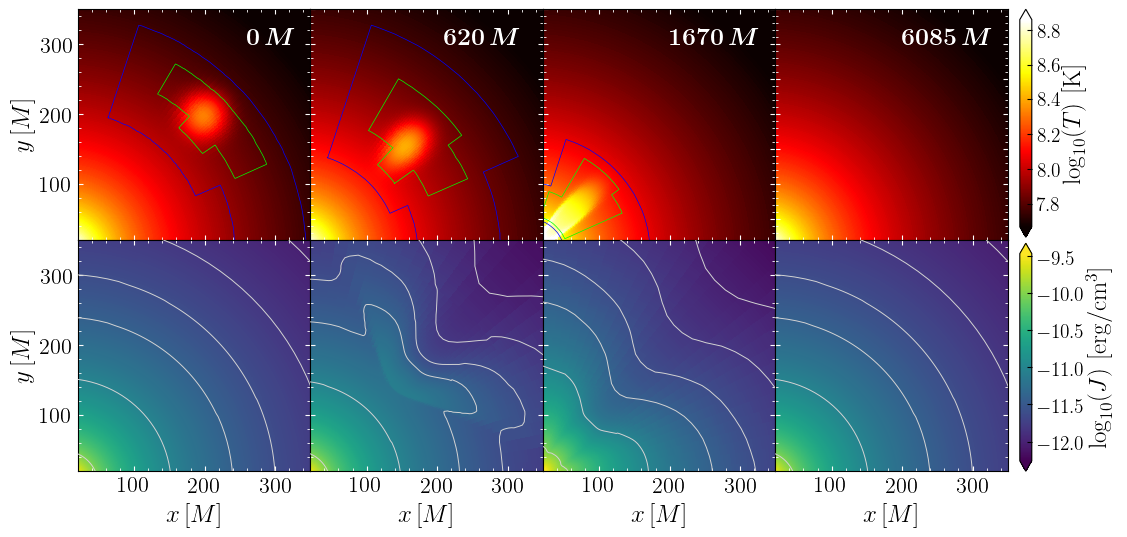
As a final test and a way to explore the stability properties of the Michel solution in the presence of a radiation field (see also Tejeda et al. 2020; Waters et al. 2020 for a related exploration in pure hydrodynamics), we next deviate from spherical symmetry via introducing a perturbation to the equilibrium solutions of Sec. 4.2. As a representative initial background configuration we consider model and introduce a perturbation in the initial temperature distribution of the form
| (102) |
where we set , and in order to fix size, amplitude and position of the perturbation, respectively. This perturbation immediately changes the density and pressure of the configuration through the equation of state, but does not affect the initial data of the radiation. The left-most panel in Fig. 14 shows the temperature (top) and the unaffected radiation-energy density (bottom) of this perturbed initial configuration. The grid extent is the same as before, with the exception that three levels of AMR are now employed. This is not just useful to resolve the temperature hot-spot introduced with the perturbation, but also to test the coupling between BHAC’s AMR routines and FRAC (see also Sec. 2.6).
The overall dynamics of the perturbed accretion problem is reported in Fig. 14. When starting the simulation, the radiation field immediately deviates from spherical symmetry (see second bottom-panel from the left) due to the increased emissivity and opacities that arise from the increased temperature around the position of the perturbation. At the same time, the underlying accretion drags the hot-spot towards the black hole (second top-panel from the left), which happens independent of the coupling to the radiation. After the hot-spot plunges into the black hole (third top-panel from left) the fluid returns to its previous equilibrium (right-most top-panel) unaffected by the radiation, whose energy is again several orders of magnitudes smaller than that of the fluid.
The radiation field (bottom panels in Fig. 14), on the other hand, shows a region of increased energy density that falls towards the black hole and at the same time a region of decreased energy density that develops behind the hot-spot. The latter region moves radially outward leading to a decreasing luminosity. The decrease in luminosity can be seen in the left panel of Fig. 15, which shows the relative difference in the bolometric luminosity with respect to the steady-state solution as a function of time. The minimum in luminosity (see ) is followed by a sharp increase with the peak luminosity at , when extracting the luminosity at . The outward propagation of the perturbation can be tracked in the right panels in Fig. 15, which show radial cuts of at an angle of and at three different times. At the beginning (top panel) and at the position of the perturbation (i.e., ), the local maximum and minimum in can be seen forming. The decrease in behind the perturbation can be interpreted as a “shadowing effect” introduced by the perturbation and hence is rather narrow in the angular direction (cf., Fig. 5). Also, while the deficit in propagates outwards at the speed of light, the corresponding increase in falls towards the black hole. When such excess in the radiation energy approaches the black hole, a ring of increased radiation energy density forms around the black hole and a part of it propagates outwards to infinity (see mid and bottom panels in Fig. 15), while another part is clearly captured by the black hole. Eventually, the radiation field returns to its initial equilibrium state. To the best of our knowledge, this is the first evidence that the radiative Michel solution is nonlinearly stable under perturbations in the radiation field.
5 Conclusions
We have implemented the moment scheme developed by Thorne 1981 (see also Rezzolla & Miller 1994; Shibata et al. 2011; Cardall et al. 2013, for numerical implementations), truncating the moment expansion at the first two moments, i.e., in what is known as the M1 scheme. The closure to the moment expansion is obtained via the Minerbo closure that – within the “grey” approximation in which the frequency dependence is integrated away – provides an accurate description of radiative transport in the optically thick and thin limits and a reasonable approximation for the intermediate regime.
Our new radiation code FRAC is logically similar to the one presented by Foucart et al. 2015, but has the important advantage of making use of an Implicit-Explicit (IMEX) IMEX scheme in order to tackle the stiffening of radiative-transfer equations in the regimes of very high opacity. Indeed, adopting this technique is essential to obtain accurate solutions at acceptable computational costs in those regimes where the absorption or scattering opacities are very large. To this scope, we have provided a systematic description of the steps necessary – and of the potential pitfalls to be encountered – when implementing a two-moment scheme within an IMEX scheme to include radiative-transfer contributions in numerical simulations of general-relativistic plasmas.
FRAC has been developed as a stand-alone code and can therefore be coupled to any other code solving the equations of GRMHD, either as on fixed or on dynamical spacetimes. This feature has allowed us to couple FRAC to BHAC, a GRMHD code recently developed to explore accretion processes onto black holes (Porth et al. 2017), and work is in progress to obtain a similar coupling with FIL (Most et al. 2019a; Most et al. 2019b). Hence, we expect that similar couplings will be possible with other codes, e.g., to those publicly available within the Einstein toolkit (Loeffler et al. 2012), when a public version of FRAC will be released.
We have shown in a number of tests, in special and general relativity, that FRAC performs well for all scenarios encountered within the simulation of accretion problems onto compact objects or the merger of binary systems of compact objects. The only exception to this successful suite of tests is represented by the crossing-beam problem, whose accurate treatment requires a different method than the one employed in this work.
As a first physically relevant application of the new code, we have simulated the problem of spherically symmetric accretion onto a nonrotating black hole, i.e., the radiative Michel solution, thus coupling FRAC with BHAC within an AMR approach. Investigating a large parameter space, we derived a simple expression [cf., Eq. (101)] that links the black-hole accretion efficiency to the three properties of the system, namely, the temperature, the bolometric luminosity and black-hole mass.
We further evaluated this accretion problem away from spherical symmetry by introducing a Gaussian perturbation in the initial temperature distribution. We found the system to return to its spherically symmetric equilibrium, which is achieved by radiating the excess energy to infinity. This process is captured faithfully in the lightcurve, which shows first a minimum produced by the shadowing effect introduced by the perturbation, followed then by a maximum resulting from the accretion of the perturbation onto the black hole. Because the system eventually recovers the stationary solution in the absence of a perturbation, this is, to the best of our knowledge, the first evidence that the radiative Michel solution is nonlinearly stable under perturbations in the radiation field.
Acknowledgements
It is a pleasure to thank Elias Most, Fabio Bacchini and Bart Ripperda for useful discussions. LRW acknowledges support from HGS-HIRe. Support also comes in part from “PHAROS”, COST Action CA16214; LOEWE-Program in HIC for FAIR; the ERC Synergy Grant “BlackHoleCam: Imaging the Event Horizon of Black Holes” (Grant No. 610058). The simulations were performed on the SuperMUC and SuperMUC-NG clusters at the LRZ in Garching, on the LOEWE cluster in CSC in Frankfurt, and on the HazelHen cluster at the HLRS in Stuttgart.
References
- Abbott et al. (2017) Abbott B. P., et al., 2017, Astrophys. J. Lett., 848, L13
- Abramowicz & Fragile (2013) Abramowicz M. A., Fragile P. C., 2013, Living Rev. Relativity, 16
- Alcubierre (2008) Alcubierre M., 2008, Introduction to Numerical Relativity. Oxford University Press, Oxford, UK, doi:10.1093/acprof:oso/9780199205677.001.0001
- Alic et al. (2012) Alic D., Moesta P., Rezzolla L., Zanotti O., Jaramillo J. L., 2012, Astrophys. J., 754, 36
- Annala et al. (2018) Annala E., Gorda T., Kurkela A., Vuorinen A., 2018, Phys. Rev. Lett., 120, 172703
- Audit et al. (2002) Audit E., Charrier P., Chièze J. P., Dubroca B., 2002, arXiv e-prints, pp astro–ph/0206281
- Baiotti & Rezzolla (2017) Baiotti L., Rezzolla L., 2017, Rept. Prog. Phys., 80, 096901
- Bauswein et al. (2017) Bauswein A., Just O., Janka H.-T., Stergioulas N., 2017, Astrophys. J. Lett., 850, L34
- Begelman (1978) Begelman M. C., 1978, Mon. Not. R. Astron. Soc., 184, 53
- Bondi (1952) Bondi H., 1952, Mon. Not. R. Astron. Soc., 112, 195
- Bovard et al. (2017) Bovard L., Martin D., Guercilena F., Arcones A., Rezzolla L., Korobkin O., 2017, Phys. Rev. D, 96, 124005
- Burgio et al. (2018) Burgio G. F., Drago A., Pagliara G., Schulze H.-J., Wei J.-B., 2018, Astrophys. J., 860, 139
- Cardall et al. (2013) Cardall C. Y., Endeve E., Mezzacappa A., 2013, Phys. Rev. D, 87, 103004
- Chael et al. (2019) Chael A., Narayan R., Johnson M. D., 2019, Monthly Notices of the Royal Astronomical Society, 486, 2873
- Coughlin et al. (2018) Coughlin M. W., Dietrich T., Margalit B., Metzger B. D., 2018, arXiv e-prints,
- Davelaar et al. (2019) Davelaar J., et al., 2019, Astron. Astrophys., 632, A2
- Dibi et al. (2012) Dibi S., Drappeau S., Fragile P. C., Markoff S., Dexter J., 2012, Mon. Not. R. Astron. Soc., 426, 1928
- Dietrich & Ujevic (2017) Dietrich T., Ujevic M., 2017, Classical and Quantum Gravity, 34, 105014
- Dionysopoulou et al. (2013) Dionysopoulou K., Alic D., Palenzuela C., Rezzolla L., Giacomazzo B., 2013, Phys. Rev. D, 88, 044020
- Event Horizon Telescope Collaboration et al. (2019a) Event Horizon Telescope Collaboration et al., 2019a, Astrophys. J. Lett., 875, L1
- Event Horizon Telescope Collaboration et al. (2019b) Event Horizon Telescope Collaboration et al., 2019b, Astrophys. J. Lett., 875, L5
- Event Horizon Telescope Collaboration et al. (2019c) Event Horizon Telescope Collaboration et al., 2019c, Astrophys. J. Lett., 875, L6
- Fernández et al. (2019) Fernández R., Tchekhovskoy A., Quataert E., Foucart F., Kasen D., 2019, Mon. Not. R. Astron. Soc., 482, 3373
- Foucart (2018) Foucart F., 2018, Mon. Not. R. Astron. Soc., 475, 4186
- Foucart et al. (2015) Foucart F., et al., 2015, Phys. Rev. D, 91, 124021
- Foucart et al. (2016a) Foucart F., et al., 2016a, Phys. Rev. D, 93, 044019
- Foucart et al. (2016b) Foucart F., O’Connor E., Roberts L., Kidder L. E., Pfeiffer H. P., Scheel M. A., 2016b, Phys. Rev. D, 94, 123016
- Foucart et al. (2018) Foucart F., Duez M. D., Kidder L. E., Nguyen R., Pfeiffer H. P., Scheel M. A., 2018, Phys. Rev. D, 98, 063007
- Fragile et al. (2012) Fragile P. C., Gillespie A., Monahan T., Rodriguez M., Anninos P., 2012, Astrophys. J., Supp., 201, 9
- Fragile et al. (2014) Fragile P. C., Olejar A., Anninos P., 2014, Astrophys. J., 796, 22
- Fujibayashi et al. (2018) Fujibayashi S., Kiuchi K., Nishimura N., Sekiguchi Y., Shibata M., 2018, Astrophys. J., 860, 64
- Galeazzi et al. (2013) Galeazzi F., Kastaun W., Rezzolla L., Font J. A., 2013, Phys. Rev. D, 88, 064009
- Gillman & Stellingwerf (1980) Gillman A. W., Stellingwerf R. F., 1980, Astrophys. J., 240, 235
- Gourgoulhon (2012) Gourgoulhon E., 2012, 3+1 Formalism in General Relativity. Lecture Notes in Physics, Berlin Springer Verlag Vol. 846, Springer, doi:10.1007/978-3-642-24525-1
- Jin & Levermore (1996) Jin S., Levermore C. D., 1996, Journal of Computational Physics, 126, 449
- Just et al. (2015) Just O., Obergaulinger M., Janka H. T., 2015, Mon. Not. R. Astron. Soc., 453, 3386
- Koeppel et al. (2019) Koeppel S., Bovard L., Rezzolla L., 2019, Astrophys. J. Lett., 872, L16
- Kuroda et al. (2016) Kuroda T., Takiwaki T., Kotake K., 2016, Astrophys. J., Supp., 222, 20
- Levermore (1984) Levermore C. D., 1984, Journal of Quantitative Spectroscopy and Radiative Transfer, 31, 149
- Levermore & Pomraning (1981) Levermore C. D., Pomraning G. C., 1981, Astrophys. J., 248, 321
- Loeffler et al. (2012) Loeffler F., et al., 2012, Class. Quantum Grav., 29, 115001
- Margalit & Metzger (2017) Margalit B., Metzger B. D., 2017, Astrophys. J. Lett., 850, L19
- McKinney et al. (2014) McKinney J. C., Tchekhovskoy A., Sadowski A., Narayan R., 2014, Mon. Not. R. Astron. Soc., 441, 3177
- Melon Fuksman & Mignone (2019) Melon Fuksman J. D., Mignone A., 2019, Astrophys. J., Supp., 242, 20
- Michel (1972) Michel F. C., 1972, Astrophys. Spa. Sci., 15, 153
- Miller et al. (2019a) Miller J. M., et al., 2019a, Phys. Rev. D, 100, 023008
- Miller et al. (2019b) Miller J. M., Ryan B. R., Dolence J. C., 2019b, Astrophys. J., Supp., 241, 30
- Minerbo (1978) Minerbo G. N., 1978, J. Quant. Spectrosc. Radiative Transfer, 20, 541
- Mizuno et al. (2018) Mizuno Y., et al., 2018, Nature Astronomy,
- Mościbrodzka et al. (2011) Mościbrodzka M., Gammie C. F., Dolence J. C., Shiokawa H., 2011, The Astrophysical Journal, 735, 9
- Most et al. (2018) Most E. R., Weih L. R., Rezzolla L., Schaffner-Bielich J., 2018, Phys. Rev. Lett., 120, 261103
- Most et al. (2019a) Most E. R., Papenfort L. J., Dexheimer V., Hanauske M., Schramm S., Stöcker H., Rezzolla L., 2019a, Physical Review Letters, 122, 061101
- Most et al. (2019b) Most E. R., Papenfort L. J., Rezzolla L., 2019b, Mon. Not. R. Astron. Soc., 490, 3588
- Murchikova et al. (2017) Murchikova E. M., Abdikamalov E., Urbatsch T., 2017, Mon. Not. R. Astron. Soc., 469, 1725
- Nobili et al. (1991) Nobili L., Turolla R., Zampieri L., 1991, Astrophys. J., 383, 250
- O’Connor (2015) O’Connor E., 2015, Astrophys. J., Supp., 219, 24
- Olivares et al. (2019) Olivares H., Porth O., Davelaar J., Most E. R., Fromm C. M., Mizuno Y., Younsi Z., Rezzolla L., 2019, Astronomy & Astrophysics, 629, A61
- Palenzuela et al. (2009) Palenzuela C., Lehner L., Reula O., Rezzolla L., 2009, Mon. Not. R. Astron. Soc., 394, 1727
- Pareschi & Russo (2005) Pareschi L., Russo G., 2005, Journal of Scientific Computing, 25, 129
- Paschalidis (2017) Paschalidis V., 2017, Classical and Quantum Gravity, 34, 084002
- Perego et al. (2014) Perego A., Rosswog S., Cabezón R. M., Korobkin O., Käppeli R., Arcones A., Liebendörfer M., 2014, Mon. Not. R. Astron. Soc., 443, 3134
- Perego et al. (2017) Perego A., Radice D., Bernuzzi S., 2017, Astrophys. J. Lett., 850, L37
- Pomraning (1981) Pomraning G. C., 1981, J. Quant. Spectrosc. Radiative Transfer, 26, 385
- Pons et al. (2000) Pons J. A., Ibáñez J. M., Miralles J. A., 2000, Mon. Not. R. Astron. Soc., 317, 550
- Porth et al. (2017) Porth O., Olivares H., Mizuno Y., Younsi Z., Rezzolla L., Moscibrodzka M., Falcke H., Kramer M., 2017, Computational Astrophysics and Cosmology, 4, 1
- Radice et al. (2013) Radice D., Abdikamalov E., Rezzolla L., Ott C. D., 2013, Journal of Computational Physics, 242, 648
- Radice et al. (2018) Radice D., Perego A., Zappa F., Bernuzzi S., 2018, Astrophys. J. Lett., 852, L29
- Rahman et al. (2019) Rahman N., Just O., Janka H. T., 2019, Mon. Not. R. Astron. Soc., 490, 3545
- Rezzolla & Miller (1994) Rezzolla L., Miller J. C., 1994, Class. Quantum Grav., 11, 1815
- Rezzolla & Zanotti (2013) Rezzolla L., Zanotti O., 2013, Relativistic Hydrodynamics. Oxford University Press, Oxford, UK, doi:10.1093/acprof:oso/9780198528906.001.0001
- Rezzolla et al. (2018) Rezzolla L., Most E. R., Weih L. R., 2018, Astrophys. J. Lett., 852, L25
- Ripperda et al. (2019) Ripperda B., et al., 2019, Astrophys. J., Supp., 244, 10
- Rivera-Paleo & Guzmán (2019) Rivera-Paleo F. J., Guzmán F. S., 2019, Astrophys. J., Supp., 241, 28
- Roedig et al. (2012) Roedig C., Zanotti O., Alic D., 2012, Mon. Not. R. Astron. Soc., 426, 1613
- Rosswog & Liebendörfer (2003) Rosswog S., Liebendörfer M., 2003, Mon. Not. R. Astron. Soc., 342, 673
- Rosswog et al. (2014) Rosswog S., Korobkin O., Arcones A., Thielemann F.-K., Piran T., 2014, Mon. Not. R. Astron. Soc., 439, 744
- Ruffert et al. (1996) Ruffert M., Janka H.-T., Schaefer G., 1996, Astron. Astrophys., 311, 532
- Ruiz et al. (2018) Ruiz M., Shapiro S. L., Tsokaros A., 2018, Phys. Rev. D, 97, 021501
- Rybicki & Lightman (1986) Rybicki G. B., Lightman A. P., 1986, Radiative Processes in Astrophysics. Wiley-VCH
- Sa̧dowski et al. (2013) Sa̧dowski A., Narayan R., Tchekhovskoy A., Zhu Y., 2013, Mon. Not. R. Astron. Soc., 429, 3533
- Sekiguchi et al. (2016) Sekiguchi Y., Kiuchi K., Kyutoku K., Shibata M., Taniguchi K., 2016, Phys. Rev. D, 93, 124046
- Shibata et al. (2011) Shibata M., Kiuchi K., Sekiguchi Y., Suwa Y., 2011, Progress of Theoretical Physics, 125, 1255
- Shibata et al. (2019) Shibata M., Zhou E., Kiuchi K., Fujibayashi S., 2019, Phys. Rev. D, 100, 023015
- Siegel & Ciolfi (2016) Siegel D. M., Ciolfi R., 2016, Astrophys. J., 819, 14
- Siegel & Metzger (2017) Siegel D. M., Metzger B. D., 2017, Physical Review Letters, 119, 231102
- Smit et al. (1997) Smit J. M., Cernohorsky J., Dullemond C. P., 1997, Astron. Astrophys., 325, 203
- Tejeda et al. (2020) Tejeda E., Aguayo-Ortiz A., Hernandez X., 2020, Astrophys. J., 893, 81
- Tews et al. (2018) Tews I., Margueron J., Reddy S., 2018, Physical Review C, 98, 045804
- The LIGO Scientific Collaboration & The Virgo Collaboration (2017) The LIGO Scientific Collaboration The Virgo Collaboration 2017, Phys. Rev. Lett., 119, 161101
- The LIGO Scientific Collaboration et al. (2017) The LIGO Scientific Collaboration et al., 2017, Astrophys. J. Lett., 848, L12
- Thorne (1981) Thorne K. S., 1981, Mon. Not. R. Astron. Soc., 194, 439
- Turner & Stone (2001) Turner N. J., Stone J. M., 2001, Astrophys. J., Supp., 135, 95
- Vitello (1978) Vitello P. A. J., 1978, Astrop. J., 225, 694
- Waters et al. (2020) Waters T., Aykutalp A., Proga D., Johnson J., Li H., Smidt J., 2020, Mon. Not. R. Astron. Soc., 491, L76
- Zampieri et al. (1996) Zampieri L., Miller J. C., Turolla R., 1996, Mon. Not. R. Astron. Soc., 281, 1183
- Zanotti et al. (2011) Zanotti O., Roedig C., Rezzolla L., Del Zanna L., 2011, Mon. Not. R. Astron. Soc., 417, 2899
Appendix A Units and units conversions
Special attention has to be paid to the system of units used when coupling radiative-transfer and GRMHD codes (see also Appendix A of Rezzolla & Zanotti 2013). Indeed, it is not uncommon to encounter tedious problems when converting quantities from the units that are routinely used in the GRMHD codes (normally employing geometrised units) and the units in which physical quantities – such as the opacities and emissivities – are routinely expressed (normally employing CGS units). BHAC, for instance, makes use of geometrised units with and it assumes that there is a stationary background metric of mass , so that all lengthscales can be scaled in terms of such a mass as , times as , and velocities as . Due to this scale invariance one can typically choose for convenience.
In the presence of radiation, however, this scale invariance is broken, because new scales are introduced by microphysical quantities, e.g., the proton mass. While is still a reasonable choice when considering matter at high densities (such as in simulations of binary neutron stars), it may lead to rest-mass densities in typical simulations of accretion problems onto supermassive black holes, thus exposing the numerical calculations to floating-point errors. To avoid this problem, we exploit the fact that the accreted mass is much smaller than that of the central black hole and thus can be neglected as a contribution for the spacetime curvature, allowing us to define an independent mass-scale for the fluid. We choose this scale via the Eddington mass-accretion rate, so that and all related quantities follow from this scaling, e.g., the rest-mass density will have dimensions . An additional advantage of this specific system of units is that the accretion rate is naturally expressed in terms of and the computed luminosity will be already rescaled in terms of the Eddington luminosity.
For easy reference, we report below some useful conversion relations for the natural constants:
| (103) | ||||
| (104) |
where the temperature unit Kelvin, i.e., , remains unchanged. The radiation constant is implemented in CGS units and enters in the computation of the emissivity. For the latter, we first express quantities in CGS units and then convert to code units via
| (105) |
Finally, the opacities are converted straightforwardly via
| (106) |