Images of point charges in conducting ellipses and prolate spheroids

Matt Majic Email: mattmajic@gmail.com Affiliation: The MacDiarmid Institute for Advanced Materials and Nanotechnology, School of Chemical and Physical Sciences, Victoria University of Wellington, PO Box 600, Wellington 6140, New Zealand

August 11, 2026

Abstract

This is an investigation into the exact forms of images of point charges in 2D conducting ellipses and 3D prolate spheroids. For an ellipse with exterior point source, we compare two previous expressions for the analytic continuation inside the ellipse down to the focal line, the location of the image charge. For an interior source, we discover a sequence of image charges lying outside. For a point source close the surface of a spheroid, series solutions for the potential diverge in a region that encompasses the singularities of the continuation of the reflected potential inside the spheroid. We uncover an image system for a point charge on the axis of a prolate spheroid that extends from the focal segment somewhat further up the axis. For an off axis charge we find a new approximate image charge. For a point charge at the center of the spheroid, the image singularity is found to lie on an infinitely wide, flat sheet with a hole around the spheroid. For a point charge located anywhere inside the spheroid, we find two new approximate image charge solutions, a point charge in real space which applies when source lies near the surface, or a point charge in complex space which projects as a ring in the real space which applies when the source lies near the rotation axis. When the point charge lies exactly on a focal point, a multipole of order 1/2 is an ideal image approximation.

I Introduction

The image solution for the electrostatic point charge near a conducting sphere is well known and consists of an image point charge located at the Kelvin inversion point. It is natural to ask how this might extend to similar analytic geometries such as the spheroid. In other words, our goal is to analytically continue Green’s function inside the spheroid as far as we can – representing the function analytically everywhere except on the smallest possible singularity, and this singularity we call the “image” of the point charge. This is equivalent to a Dirichlet problem where an analytic function must be found that has the $1/r$ singularity in the vicinity of the point charge and is zero on the boundary of the spheroid. The first exact formulation of the image of a point charge on the axis of a spheroid was in 1995 - partial success was found by Sten and Lindell sten1995electrostatic where the image consisted of a line charge lying on the focal segment. A later investigation of the image solution for the elliptic cylinder sten1996focal, revealed that the image lies on a focal strip, but if the source is close enough, a disjoint point image must be added to the image system. In fact the potential computed by this image system gives the full analytic continuation of the potential. In this sense the image is what we will call “reduced”, meaning the singularities occupy the smallest or a vanishingly small spatial domain. But for the spheroid, the authors of sten1995electrostatic later realized that their expression for the image diverges when the point charge is too close to the surface lindell2001electrostatic, and attempted to amend the image solution by subtracting an image point charge, but unlike the case of the elliptic cylinder, this proposed image system does not work - the series for the image charge density on the focal segment still diverges. The authors later studied the same problem for the dielectric spheroid lindell2001dielectric and used an approximate correction by extending the image from (and including) the focal segment up to the location of the point image, to imitate the line image for the dielectric sphere. For the non-rotational ellipsoid, the first proposed image solution consisted of a point charge plus a surface charge on an interior ellipsoid dassios2009image. This image formulation was then presented for the particular case of the prolate spheroid in Xue2017. But the spheroidal surface charge image cloaks a reduced image lying inside. For the non-rotational ellipsoid with Neumann boundary condition, the first attempt at finding an image solution is in dassios2012neumann, where they assumed a point image plus a curved line of image charge extending along a spheroidal coordinate line, but they still needed to correct for this by adding a surface charge on an ellipsoidal surface that encloses the point and line image. This image formulation is specialized for the prolate spheroid in xue2018image. A recent paper alshal2018image suggested that the best image solution may be to use Sommerfeld images which are placed in a second copy of $\mathbb{R}^{3}$ , attached at the surface.

There has also been a separate vein of research into the analytic continuation of solutions of more general Dirichlet boundary problems with particular attention to ellipsoids, see for example khavinson2010search.

Here we attempt to find the reduced form of the image of a point charge near or inside a conducting spheroid. First in section II we cover the 2D analogue of an elliptic cylinder, and find exact image solutions for point sources located outside and inside the ellipse. These images are used as hints for the image locations in prolate spheroids. Section III covers the progress made by lindell2001electrostatic for the point charge on the rotation axis. We then devise a series expansion by geometric transformations that uncovers the true form of the image. In section III.5 we speculate about the form of the image system for a point charge located off the rotation axis, and find a simple approximate image point charge which is a generalization of the axial case, and a correction is made to a claim regarding convergence of the double series from an earlier version of the manuscript majic2021imagespheroid. In section IV.1 we investigate the similar problem of a point charge at the center of a prolate spheroid, constructing a series solution that suggests the reduced image lies on an infinitely wide, flat sheet with a hole around the spheroid. In section IV the source charge is placed anywhere inside the spheroid, and two approximate image solutions are found, depending on the location of the source. When the source is located exactly on a focal point, we find that the image is approximately represented by a multipole of order 1/2.

II Elliptic cylinder - 2D

Electrostatics problems in 2D are more suited to solving via image charges, so we study the ellipse as a precursor to the spheroid.

Physically this problem represents a conducting elliptic cylinder in the presence of an infinite parallel line source. We will refer to the problem as if it were completely 2 dimensional, consisting of a conducting ellipse in the presence of a point charge.

The elliptic coordinate system is built around a focal line of length $2f$ lying on $-f\leq x\leq f$ , $y=0$ , where $x,y$ are Cartesian coordinates. The elliptic coordinates $\xi,\eta$ are defined as

	$\displaystyle\cosh\xi$	$\displaystyle=\frac{\sqrt{(x+f)^{2}+y^{2}}+\sqrt{(x-f)^{2}+y^{2}}}{2f},\qquad$	$\displaystyle x$	$\displaystyle=f\cosh\xi\cos\eta,$
	$\displaystyle\cos\eta$	$\displaystyle=\frac{\sqrt{(x+f)^{2}+y^{2}}-\sqrt{(x-f)^{2}+y^{2}}}{2f},\qquad$	$\displaystyle y$	$\displaystyle=f\sinh\xi\sin\eta,$		(1)

with $\xi\in[0,\infty)$ describing confocal ellipses around the focus and $\eta\in[0,2\pi)$ describing semi-hyperbolas. $\xi=0$ corresponds to the focal strip and $\xi$ increases with the distance from the origin $\rho=\sqrt{x^{2}+y^{2}}$ . The conducting ellipse is defined by $\xi=\xi_{0}$ . The 2D Laplacian is separable in this coordinate system and the corresponding solutions are the elliptic cylindrical harmonics. The interior harmonics are

\displaystyle\cosh(n\xi)\cos(n\eta),\qquad\sinh(n\xi)\sin(n\eta)

(2)

which are regular at the focus but increase exponentially as $\rho\rightarrow\infty$ , so are used to expand interior potentials. And the exterior elliptic cylindrical harmonics are

\displaystyle e^{-n\xi}\cos(n\eta),\qquad e^{-n\xi}\sin(n\eta)

(3)

which are singular on the focus but decay as $\rho\rightarrow\infty$ .

II.1 external line charge

Figure 1: schematic of the image solution for a line charge near a 2d elliptic cylinder.

A complete reduced image solution was derived by Sten sten1996focal for a source outside a conducting or dielectric ellipse. This section briefly covers the derivations and describes the image for the conducting case.

The problem is to solve for the potential outside the ellipse $V$ , which behaves as the point source in its vicinity, is zero on the ellipse (Dirichlet boundary condition), and decays to 0 as $\rho\rightarrow\infty$ . To do this we write $V=V_{e}+V_{r}$ where $V_{e}$ is the known excitation - the potential of the point charge with no ellipse, and $V_{r}$ is the potential reflected by the ellipse which is to be solved. The source lies at $(x,y)=(x_{d},y_{d})$ , or $(\xi,\eta)=(\xi_{d},\eta_{d})$ , and its potential may be expanded in elliptical harmonics for $\xi<\xi_{d}$ as

	$\displaystyle V_{e}$	$\displaystyle=\log\frac{f}{\sqrt{(x-x_{d})^{2}+(y-y_{d})^{2}}}$
		$\displaystyle=-\xi_{0}+\log 2+\sum_{n=1}^{\infty}\frac{2}{n}e^{-n\xi_{d}}\big[\cosh(n\xi)\cos(n\eta_{d})\cos(n\eta)+\sinh(n\xi)\sin(n\eta_{d})\sin(n\eta)\big].$		(4)

To solve for $V_{r}$ , it is expanded as a series of exterior harmonics $e^{-n\xi}[A_{n}\cos(n\eta)+B_{n}\sin(n\eta)]$ , where $A_{n}$ , $B_{n}$ are chosen to satisfy the boundary condition $V_{r}+V_{e}=0$ at $\xi=\xi_{0}$ , giving

\displaystyle V_{r}=\xi-\xi_{0}+\xi_{d}-\log 2-\sum_{n=1}^{\infty}\frac{2}{n}e^{n(\xi_{0}-\xi_{d}-\xi)}\big[\cosh(n\xi_{0})\cos(n\eta_{d})\cos(n\eta)+\sinh(n\xi_{0})\sin(n\eta_{d})\sin(n\eta)\big].

(5)

The terms before the sum only affect the charge of the ellipse and the zero of the potential, and have been chosen so that $V_{r}$ coincides with a later expression. While the physical potential is equal to zero inside the ellipse, the series for $V_{r}$ converges all the way down to the focal line if the source is far enough such that $\xi_{d}>2\xi_{0}$ , hence Eq. (5) may be identified with the potential of a charge distribution on the focal strip. The exact charge distribution may be found using the following representations of elliptical harmonics:

$\displaystyle\xi-\log(2)=$	$\displaystyle\frac{1}{\pi}\int_{-f}^{f}\frac{-1}{\sqrt{f^{2}-x^{\prime 2}}}\log\frac{f}{\sqrt{(x-x^{\prime})^{2}+y^{2}}}\mathrm{d}x^{\prime}$			(6)
$\displaystyle e^{-n\xi}\cos(n\eta)=$	$\displaystyle\frac{n}{\pi}\int_{-f}^{f}\frac{T_{n}(x^{\prime}/f)}{\sqrt{f^{2}-x^{\prime 2}}}\log\frac{f}{\sqrt{(x-x^{\prime})^{2}+y^{2}}}\mathrm{d}x^{\prime}\qquad$	$\displaystyle n$	$\displaystyle\geq 1$	(7)
$\displaystyle e^{-n\xi}\sin(n\eta)=$	$\displaystyle\frac{-1}{f\pi}\int_{-f}^{f}U_{n-1}(x^{\prime}/f)\sqrt{f^{2}-x^{\prime 2}}\frac{\partial}{\partial y}\log\frac{f}{\sqrt{(x-x^{\prime})^{2}+y^{2}}}\mathrm{d}x^{\prime}.\qquad$	$\displaystyle n$	$\displaystyle\geq 1$	(8)

Eq. (6) is an integral over a charge distribution on the focus, concentrated towards the ends, Eq. (7) is a charge distribution of a Chebyshev polynomial of the first kind $T_{n}$ , and (8) is a distribution of dipoles pointing in the $y$ direction weighted by a Chebyshev polynomial of the second kind $U_{n-1}$ . Inserting these into Eq. (5) allows us to express $V_{r}$ as the potential of image charges and dipoles on the focal strip:

\displaystyle V_{r}=\xi_{d}-\xi_{0}-\int_{-f}^{f}\bigg[q(x^{\prime})\log\frac{f}{\sqrt{(x-x^{\prime})^{2}+y^{2}}}+p(x^{\prime})\frac{\partial}{\partial y}\log\frac{f}{\sqrt{(x-x^{\prime})^{2}+y^{2}}}\bigg]\mathrm{d}x^{\prime}

(9)

where the charge distribution $q$ and dipole layer distribution $p$ are

	$\displaystyle q(x)$	$\displaystyle=\frac{f}{\pi\sqrt{f^{2}-x^{2}}}\left(1+2\sum_{n=0}^{\infty}e^{n(\xi_{0}-\xi_{d})}\cosh(n\xi_{0})\cos(n\eta_{d})T_{n}(x/f)\right)$		(10)
	$\displaystyle p(x)$	$\displaystyle=-\frac{\sqrt{f^{2}-x^{2}}}{\pi f}\sum_{n=1}^{\infty}\frac{2}{n}e^{n(\xi_{0}-\xi_{d})}\sinh(n\xi_{0})\sin(n\eta_{d})U_{n-1}(x/f).$		(11)

But if the source is too close such that $\xi_{d}<2\xi_{0}$ , these series diverge. To amend this, a point image source may be extracted with the correct charge and position, to make the remaining series converge all the way down to the focal strip. This image lies at $\xi=\xi_{h}=2\xi_{0}-\xi_{d}$ , $\eta=\eta_{d}$ ( $x=x_{h},y=y_{h}$ ) with opposite magnitude to the source, and has potential $V_{h}$ with the following expansion:

	$\displaystyle V_{h}$	$\displaystyle=\xi+\log 2-\log\frac{f}{\sqrt{(x-x_{h})^{2}+(y-y_{h})^{2}}}$		(12)
		$\displaystyle=-\sum_{n=1}^{\infty}\big[\cosh(n\xi_{h})\cos(n\eta_{d})\cos(n\eta)+\sinh(n\xi_{h})\cos(n\eta_{d})\cos(n\eta)\big]\frac{2}{n}e^{-n\xi}.\qquad\xi>\xi_{h}$		(13)

Note that $V_{h}$ has zero monopole moment due to the $\xi$ term. By adding $V_{h}$ in the form (12) to $V_{r}$ and subtracting the form (13), we get a series for $V_{r}$ that converges down to the focal strip:

$\displaystyle V_{r}(\xi_{d}>2\xi_{0})=~$	$\displaystyle\xi_{d}-\xi_{0}-\log\frac{f}{\sqrt{(x-x_{h})^{2}+(y-y_{h})^{2}}}$
	$\displaystyle-\sum_{n=1}^{\infty}\frac{2}{n}\bigg(\big[e^{n(\xi_{0}-\xi_{d})}\cosh(n\xi_{0})-\cosh(n\xi_{h})\big]\cos(n\eta_{d})\cos(n\eta)$
	$\displaystyle\hskip 28.45274pt+\big[e^{n(\xi_{0}-\xi_{d})}\sinh(n\xi_{0})-\sinh(n\xi_{h})\big]\sin(n\eta_{d})\sin(n\eta)\bigg)e^{-n\xi}$	(14)

which corresponds to the image system if $\xi_{d}\leq 2\xi_{0}$ :

$\displaystyle q_{h}(x,y)$	$\displaystyle=-\delta(x-x_{h})\delta(y-y_{h})$	(15)
$\displaystyle q(x)$	$\displaystyle=\frac{2f}{\pi\sqrt{f^{2}-x^{2}}}\sum_{n=1}^{\infty}\big[e^{n(\xi_{0}-\xi_{d})}\cosh(n\xi_{0})-\cosh(n\xi_{h})\big]\cos(n\eta_{d})T_{n}(x/f)$	(16)
$\displaystyle p(x)$	$\displaystyle=-\frac{\sqrt{f^{2}-x^{2}}}{\pi f}\sum_{n=1}^{\infty}\frac{1}{n}\big[e^{n(\xi_{0}-\xi_{d})}\sinh(n\xi_{0})-\sinh(n\xi_{h})\big]\sin(n\eta_{d})U_{n-1}(x/f)$	(17)

These images are depicted schematically in Figure 1, and the potential is plotted in Figure 2. The potential of these images is the analytic continuation of $V_{r}$ to all space.

In two-dimensions analytic continuation of solutions to Dirichlet problems is much more tractable for many geometries, using a wide range of conformal mappings, or the Schwarz function bell2006classical. In the next section we look at an elegant approach using reflection alshal2021image which provides a closed form expression for the image.

Refer to caption — Figure 2: Analytic continuation of the potential $V_{\rm out}=V_{e}+V_{r}$ of a point source outside an ellipse (green) with $f=1$ , $\xi_{0}=0.6$ , $\xi_{d}=0.79$ , $\eta_{d}=0.96$ , computed via either series or the Kelvin image approach.

II.2 Alternate method

The same problem of a point source outside a conducting ellipse is solved in Ref. alshal2021image via the Kelvin and Sommerfeld image methods, and these methods give simple expressions for the analytic continuation of the potential. The two methods essentially obtain the same expression, so we just reproduce the Kelvin method here.

The approach uses a function $G$ , similar to Green’s function of an isolated point source, but where $\mathbb{R}^{2}$ is replaced by a double surface attached at the focal line curtright2018conducting:

\displaystyle G(\xi,\eta,\xi_{d},\eta_{d})=-\frac{1}{2}|\xi-\xi_{d}|-\frac{1}{2}\log\big(1-e^{-2|\xi-\xi_{d}|}+2e^{-|\xi-\xi_{d}|}\cos(\eta-\eta_{d})\big).

(18)

$G$ may also be viewed as the potential of a point charge plus a charge distribution on the focal strip. To construct a solution $V$ to Laplace’s equation that is zero on the boundary of the ellipse $\xi_{0}$ , one simply takes the difference of two offset copies of $G$ as

\displaystyle V=G(\xi,\eta,\xi_{d},\eta_{d})-G(\xi,\eta,\xi_{h},\eta_{d}).

(19)

where again $\xi_{h}=2\xi_{0}-\xi_{d}$ is the $\xi$ parameter of the image point source (note $\xi_{h}<0$ is allowed and corresponds to the point source lying in the second copy of $\mathbb{R}^{2}$ ). Note that the first term in (19) is not just the source and the second term is not the complete image, because both contribute towards image charges on the focal segment. To be explicit, the reflected potential is $V_{r}=V-V_{e}$ , which gives the closed form of the series solution (5).

A closed form of the image charge and dipole distributions can be found by evaluating the electric field at the focal strip. The image charge distribution causes a discontinuity in the electric field crossing the focal strip:

\displaystyle\left.\frac{\partial V}{\partial y}\right|_{y\rightarrow 0^{+}}-\left.\frac{\partial V}{\partial y}\right|_{y\rightarrow 0^{-}}=2\pi q(x)

(20)

And the image dipole layer causes a discontinuity in the potential across the focal strip:

\displaystyle V(x,y\rightarrow 0^{+})-V(x,y\rightarrow 0^{-})=2\pi p(x)

(21)

Using these with the potential Eq. (19) gives alternative but equivalent expressions to those in Eqs. (11,10) if $\xi_{d}\geq 2\xi_{0}$ , or (17,16) if $\xi_{d}<2\xi_{0}$ :

$\displaystyle q(x)=$	$\displaystyle\frac{f}{4\pi\sqrt{f^{2}-x^{2}}}\bigg[\frac{\sinh\xi_{d}}{\cosh\xi_{d}-\cos(\eta_{d}+\text{acos}(x/f))}-\frac{\sinh\xi_{h}}{\cosh\xi_{h}-\cos(\eta_{d}+\text{acos}(x/f))}$
	$\displaystyle\hskip 56.9055pt+\frac{\sinh\xi_{d}}{\cosh\xi_{d}-\sin(\eta_{d}+\text{asin}(x/f))}-\frac{\sinh\xi_{h}}{\cosh\xi_{h}-\sin(\eta_{d}+\text{asin}(x/f))}\bigg]$	(22)
$\displaystyle p(x)=$	$\displaystyle\frac{1}{4\pi}\bigg[\log\frac{\cosh\xi_{d}+\sin(\eta_{d}-\text{asin}(x/f))}{\cosh\xi_{d}-\sin(\eta_{d}+\text{asin}(x/f))}-\log\frac{\cosh\xi_{h}+\sin(\eta_{d}-\text{asin}(x/f))}{\cosh\xi_{h}-\sin(\eta_{d}+\text{asin}(x/f))}\bigg].$	(23)

These expressions do not depend on whether the image point source is present (i.e. if $\xi_{d}<2\xi_{0}$ ), despite the absolute value signs $|\xi-\xi_{h}|$ appearing in (19). Figure 3 shows that $q(x)$ varies smoothly as $\xi_{d}$ crosses $2\xi_{0}$ , while $p(x)$ has an unbounded peak for $\xi_{d}=2\xi_{0}$ .

Ref. alshal2021image suggests that this type of image solution could generalize to spheroids, although surely the generalization would be much more complicated, and we can’t reproduce the result.

Figure 3: Charge density

q

(left) and dipole density

p

(right) for a 2D point charge outside an ellipse with

\xi_{0}=0.6

\eta_{d}=.96

(same as in Fig. 2), and a range of

\xi_{d}

including

\xi_{d}=2\xi_{0}

II.3 Source at center

The problem of a point source inside a conducting ellipse appears to have attracted no attention. So here we solve the problem and determine the image outside the ellipse, starting with the simple case of a point source placed at the origin. The potential of the line charge should be expanded as

	$\displaystyle V_{e}$	$\displaystyle=\log\frac{f}{\rho}$
		$\displaystyle=-\xi+\log 2+\sum_{n=1}^{\infty}\frac{2}{n}e^{-n\xi}\cos\frac{n\pi}{2}\cos n\eta$		(24)

and the reflected potential is expanded on a series of $\cosh n\xi\cos(n\eta)$ which are smooth inside the ellipse:

\displaystyle V_{r}=\xi_{0}-\log 2-\sum_{n=1}^{\infty}\frac{2}{n}\frac{e^{-n\xi_{0}}}{\cosh(n\xi_{0})}\cosh(n\xi)\cos\frac{n\pi}{2}\cos n\eta.

(25)

Just like for the external point source, we want to extract the most significant contributions (leading order with respect to $n$ ) from the series. In fact the following series expansion gives all orders in $n$ :

	$\displaystyle\frac{e^{-n\xi_{0}}}{\cosh(n\xi_{0})}=$	$\displaystyle-2e^{-2n\xi_{0}}+2e^{-4n\xi_{0}}-2e^{-6n\xi_{0}}+...$
	$\displaystyle=$	$\displaystyle 2\sum_{k=1}^{\infty}(-)^{k}e^{-2kn\xi_{0}}\qquad\xi_{0}>0.$		(26)

The sum over $n$ of the $k^{th}$ term gives two identical point sources at $x=0,~y_{k}=\pm\sinh(2k\xi_{0})$ (plus a constant term), so $V_{r}$ can be represented as a series of point charges of alternating sign whose spacing increases with distance from the ellipse:

\displaystyle V_{r}=\xi_{0}-\log 2+\sum_{k=1}^{\infty}(-)^{k}\bigg(4k\xi_{0}-2\log 2+\log\frac{f}{\sqrt{x^{2}+(y-y_{k})^{2}}}+\log\frac{f}{\sqrt{x^{2}+(y+y_{k})^{2}}}\bigg).

(27)

The analytic continuation of the potential $V_{e}+V_{r}$ is plotted in Fig. 4 using Eq. (27), revealing the image charges. The image problem of a point charge at the center of a spheroid is much more complex as seen in section IV.1.

II.4 Internal source off center

This problem is also solvable with a relatively simple image system. The excitation is

	$\displaystyle V_{e}$	$\displaystyle=\log\frac{f}{\sqrt{(x-x_{d})^{2}+(y-y_{d})^{2}}}$
		$\displaystyle=-\xi+\log 2+\sum_{n=1}^{\infty}\frac{2}{n}e^{-n\xi}\big[\cosh(n\xi_{d})\cos(n\eta_{d})\cos(n\eta)+\sinh(n\xi_{d})\sin(n\eta_{d})\sin(n\eta)\big]$		(28)

and $V_{r}$ is found to be

\displaystyle V_{r}=\xi_{0}-\log 2-\sum_{n=1}^{\infty}\frac{2}{n}e^{-n\xi_{0}}\bigg[\frac{\cosh(n\xi_{d})}{\cosh(n\xi_{0})}\cosh(n\xi)\cos(n\eta_{d})\cos(n\eta)+\frac{\sinh(n\xi_{d})}{\sinh(n\xi_{0})}\sinh(n\xi)\sin(n\eta_{d})\sin(n\eta)\bigg].

(29)

Here we can expand the series coefficients as

	$\displaystyle e^{-n\xi_{0}}\frac{\cosh(n\xi_{d})}{\cosh(n\xi_{0})}$	$\displaystyle=-(e^{n\xi_{d}}+e^{-n\xi_{d}})\sum_{k=1}^{\infty}(-)^{k}e^{-2kn\xi_{0}}$
	$\displaystyle e^{-n\xi_{0}}\frac{\sinh(n\xi_{d})}{\sinh(n\xi_{0})}$	$\displaystyle=(e^{n\xi_{d}}-e^{-n\xi_{d}})\sum_{k=1}^{\infty}e^{-2kn\xi_{0}}$		(30)

A reasonable guess for the image system would be a series of point charges similar to those found in the previous section. Towards associating the series with expansions of point sources we organize the series for $V_{r}$ in to two parts, with $e^{n\xi_{0}}$ or $e^{-n\xi_{0}}$ :

	$\displaystyle V_{r}=\xi_{0}-\log 2+\sum_{k=1}^{\infty}\bigg\{$	$\displaystyle\sum_{n=1}^{\infty}\frac{2}{n}e^{-n(2k\xi_{0}+\xi_{d})}\big[(-)^{k}\cosh(n\xi)\cos(n\eta_{d})\cos(n\eta)-\sinh(n\xi)\sin(n\eta_{d})\sin(n\eta)\big]$
	$\displaystyle+$	$\displaystyle\sum_{n=1}^{\infty}\frac{2}{n}e^{-n(2k\xi_{0}-\xi_{d})}\big[(-)^{k}\cosh(n\xi)\cos(n\eta_{d})\cos(n\eta)+\sinh(n\xi)\sin(n\eta_{d})\sin(n\eta)\big]\bigg\}.$		(31)

By adding constants, these can be identified with expansions of point sources at $(\xi,\eta)=(2k\xi_{0}\pm\xi_{d},\pm\eta_{d})$ , leading to the image formulation

\displaystyle V_{r}=\sum_{k=1}^{\infty}(-)^{k}\bigg[4k\xi_{0}-2\log 2+\log\frac{f}{\sqrt{(x-x_{k+})^{2}+(y-y_{k+})^{2}}}+\log\frac{f}{\sqrt{(x-x_{k-})^{2}+(y-y_{k-})^{2}}}\bigg]

(32)

where the coordinates of the image point charges are

\displaystyle x_{k\pm}=f\cosh(2k\xi_{0}\pm\xi_{d})\cos\eta_{d},\qquad y_{k+\pm}=f\pm(-)^{k}\sinh(2k\xi_{0}\pm\xi_{d})\sin\eta_{d}.

(33)

The analytic continuation of the total potential is plotted in Figure 5 using Eq. (32). The point charges lie on the hyperbola $\cos\eta=\cos\eta_{d}$ with alternating sign and alternating spacing that increases exponentially going further out. Numerically the total potential is also zero on infinitely many larger confocal ellipses. As $\xi_{d}\rightarrow 0,\eta_{d}\rightarrow\pi/2$ the image reduces to that for the source at the center, studied in the previous section. As the ellipse becomes more circular, all except one image charge move out towards infinity, recovering the image solution for the circle. For a charge off center but on the focal strip, the images group in twos either side of the $x$ -axis as shown in figure 6. For a charge off the focal strip, on the $x$ -axis near the tip, the images combine and line up on the $x$ -axis as shown in figure 7.

This concludes the 2D section of the paper, for which we could find the full analytic continuation in every case. These image systems should provide hints for the image locations in the 3D problem in the next sections.

III Point charge on axis of conducting prolate spheroid

Consider a conducting prolate spheroid of half-focal length $f$ , half-height $c$ and half-width $a=\sqrt{c^{2}-f^{2}}$ , where in Cartesian coordinates $x,y,z$ the rotation axis is aligned with $z$ . The spheroid is excited by a point charge located a distance $d$ up the $z$ -axis, as depicted in Figure 8. We will use spheroidal coordinates $\xi,\eta$ , with $\rho=\sqrt{x^{2}+y^{2}}$ , defined as: NIST:DLMF

Spheroidal coordinates $\xi,\eta$ are analogous to elliptic coordinates, but here we do not use the trigonometric representations:

	$\displaystyle\xi$	$\displaystyle=\frac{\sqrt{\rho^{2}+(z+f)^{2}}+\sqrt{\rho^{2}+(z-f)^{2}}}{2f},$	$\displaystyle z$	$\displaystyle=f\xi\eta,$
	$\displaystyle\eta$	$\displaystyle=\frac{\sqrt{\rho^{2}+(z+f)^{2}}-\sqrt{\rho^{2}+(z-f)^{2}}}{2f},$	$\displaystyle\rho$	$\displaystyle=f\sqrt{\xi^{2}-1}\sqrt{1-\eta^{2}}.$

Surfaces of constant $\xi$ are concentric prolate spheroids, with $\xi=1$ being the focal line, and surfaces of constant $\eta$ are hyperboloids which describe an analogue of the latitudinal angle on a given spheroid. The boundary of the spheroid is $\xi=\xi_{0}=c/f$ . The exciting potential $V_{e}$ can be expressed as a series of spheroidal harmonics:

\displaystyle V_{e}=\frac{f}{\sqrt{\rho^{2}+(z-d)^{2}}}=\sum_{n=0}^{\infty}(2n+1)Q_{n}(\xi_{d})P_{n}(\xi)P_{n}(\eta).\qquad\xi<\xi_{d}

(34)

Where $P_{n}$ and $Q_{n}$ are the Legendre functions of the first and second kinds, and $\xi_{d}=d/f$ is the $\xi$ coordinate of the source charge. We split the total potential outside the spheroid as $V=V_{e}+V_{r}$ where $V_{r}$ is the reflected potential¹¹ 1 the terminology “reflected potential” is not intended to suggest the existence of a reflection law as for example with Kelvin’s method for the sphere. by the presence of the spheroid, and the boundary condition is then $V=0$ at $\xi=\xi_{0}$ . Using the standard separation of variables approach, $V_{r}$ is found to be

\displaystyle V_{r}=-\sum_{n=0}^{\infty}(2n+1)\frac{P_{n}(\xi_{0})}{Q_{n}(\xi_{0})}Q_{n}(\xi_{d})Q_{n}(\xi)P_{n}(\eta).

(35)

We will now investigate the analytic continuation of the series (35) inside the spheroid.

III.1 Summary of progress in Ref. lindell2001electrostatic - leading order approximation and series acceleration

Figure 8: Schematic of a point charge near a prolate spheroid, showing the extended image singularity in the case of a close source charge, and the boundary of the domain of convergence of the series (35),

\xi=\xi_{h}

. Red represents positive charge and blue negative.

The Legendre functions behave for large $n$ with $m$ fixed, $x>1$ as

	$\displaystyle P_{n}^{m}(x)\rightarrow$	$\displaystyle~\sqrt{\frac{1}{2\pi}}\frac{(x+\sqrt{x^{2}-1})^{n+1/2}}{(x^{2}-1)^{1/4}}n^{m-1/2}\left[1-\frac{2m-1}{8n}\left(\frac{(2m+1)x}{\sqrt{x^{2}-1}}-2\right)+\mathcal{O}(n^{-2})\right]\qquad~~\|x\|>1$		(36)
	$\displaystyle Q_{n}^{m}(x)\rightarrow$	$\displaystyle~\sqrt{\frac{\pi}{2}}\frac{(x+\sqrt{x^{2}-1})^{-n-1/2}}{(x^{2}-1)^{1/4}}n^{m-1/2}\left[1+\frac{2m-1}{8n}\left(\frac{(2m+1)x}{\sqrt{x^{2}-1}}+2\right)+\mathcal{O}(n^{-2})\right]\qquad~~\|x\|>1$		(37)

which are modified expressions from nemes2020large. For now we are just interested in the leading order and $m=0$ , where the terms in the series (35) behave for large $n$ as

\displaystyle\frac{P_{n}(\xi_{0})}{Q_{n}(\xi_{0})}Q_{n}(\xi_{d})=\frac{1}{\sqrt{2\pi n}(\xi_{d}^{2}-1)^{1/4}}\left(\frac{\Big(\xi_{0}+\sqrt{\xi_{0}^{2}-1}\Big)^{2}}{\xi_{d}+\sqrt{\xi_{d}^{2}-1}}\right)^{n}\big[1+\mathcal{O}(n^{-1})\big].

(38)

If the point source is further than a critical distance, $d>d_{c}$ where

\displaystyle d_{c}=2\frac{c^{2}}{f}-f=f(2\xi_{0}^{2}-1),

(39)

then the series (35) converges in all space except the focal segment. The corresponding image line charge distribution $\lambda$ can be found by applying the Havelock formula havelock1952moment(p. 130) which expresses each spheroidal harmonic in terms of a charge distribution of a Legendre polynomial on the focal segment:

\displaystyle Q_{n}(\xi)P_{n}(\eta)=\frac{1}{2}\int_{-f}^{f}\frac{P_{n}(z^{\prime})}{\sqrt{\rho^{2}+(z-z^{\prime})^{2}}}\mathrm{d}z^{\prime}.

(40)

Combining this with Eq. (35) reveals the line charge density of the image:

\displaystyle\lambda(z)=-\frac{1}{2}\sum_{n=0}^{\infty}(2n+1)\frac{P_{n}(\xi_{0})}{Q_{n}(\xi_{0})}Q_{n}(\xi_{d})P_{n}(z/f),\qquad|z|<f

(41)

so that the reflected potential may be expressed in its image representation as

\displaystyle V_{r}=\int_{-f}^{f}\frac{\lambda(z^{\prime})}{\sqrt{\rho^{2}+(z-z^{\prime})^{2}}}\mathrm{d}z^{\prime}

(42)

which converges if $d>d_{c}$ . But for $d<d_{c}$ , the series (35) diverges inside the spheroid $\xi<\xi_{h}$ where

\displaystyle\xi_{h}=(2\xi_{0}^{2}-1)\xi_{d}-2\xi_{0}\sqrt{\xi_{0}^{2}-1}\sqrt{\xi_{d}^{2}-1}.

(43)

To work around this, the authors noted that the leading order of the series terms in (38) is similar to that for the spheroidal harmonic expansion of a point charge on the z-axis at $z=h=f\xi_{h}$ :

$\displaystyle V^{(0)}=$	$\displaystyle\frac{q_{h}f}{\sqrt{\rho^{2}+(z-h)^{2}}}$	(44)
$\displaystyle=$	$\displaystyle q_{h}\sum_{n=0}^{\infty}(2n+1)P_{n}(\xi_{h})Q_{n}(\xi)P_{n}(\eta),$	(45)
$\displaystyle\text{where }~~q_{h}=$	$\displaystyle-\sqrt[4]{\frac{h^{2}-f^{2}}{d^{2}-f^{2}}}.$

This is the blue dot in Figure 8. Then (45) was extracted from the series (35) so that the remaining series converged faster:

\displaystyle V\equiv V^{\prime}=V_{e}+V^{(0)}-\sum_{n=0}^{\infty}(2n+1)\bigg(\frac{P_{n}(\xi_{0})}{Q_{n}(\xi_{0})}Q_{n}(\xi_{d})+q_{h}P_{n}(\xi_{h})\bigg)Q_{n}(\xi)P_{n}(\eta).

(46)

However, the authors incorrectly assumed that the remaining image lies on the focal segment, and attempted to write down the image charge density on this strip for $d<d_{c}$ as:

\displaystyle\lambda(z)\neq-\frac{1}{2}\sum_{n=0}^{\infty}(2n+1)\bigg(\frac{P_{n}(\xi_{0})}{Q_{n}(\xi_{0})}Q_{n}(\xi_{d})+q_{h}P_{n}(\xi_{h})\bigg)P_{n}(z/f),\qquad|z|<f

(47)

but the terms increase exponentially as $n\rightarrow\infty$ and the series diverges. Ref. lindell2001electrostatic states that this series is asymptotic, initially converging then diverging, but no charge distribution confined to this segment could solve the boundary problem. In order for the potential created by this charge distribution on the focal segment to equal $V_{r}$ in any open region, it must be equal to $V_{r}$ $everywhere$ due to the identity theorem lebl2019tasty. This is not possible because $V_{r}$ also tends to infinity near $\rho=0,~f<z<h$ (see Section III.3) and this behavior cannot be reproduced by any charge distribution confined to $-f\leq z\leq f$ .

If $d>d_{c}$ then the image point charge lies off the focal segment, and is in a sense absorbed into the image line charge distribution $\lambda(z)$ . As noted in Ref. lindell2001electrostatic, extracting the image charge $V^{(0)}$ only improves the rate of convergence if $d>d_{c}$ .

III.2 Comparison to approach in Ref. Xue2017

Figure 9: Comparison of the height

h

of the image point charge in lindell2001electrostatic to that from Xue2017. The height is plotted as a function of the source charge height

d

, for two spheroids of very different aspect ratio. The top of the focal segment lies at

f=1

, and

d_{c}

is the critical height for the source charge - the blue line is only used for

d<d_{c}

In Ref. Xue2017 the authors separated out a different image point charge, where its location and strength were chosen so as to cancel out just the $n=0$ and $n=1$ terms of the series (35) exactly. They used for the height and charge:

\displaystyle h_{x}=c\frac{Q_{0}(\xi_{0})Q_{1}(\xi_{d})}{Q_{1}(\xi_{0})Q_{0}(\xi_{d})},\qquad q_{x}=c\frac{Q_{0}(\xi_{d})}{Q_{0}(\xi_{0})}.

(48)

As shown in Fig. 9, the height of the image $h_{x}$ in Ref. Xue2017 decreases all the way to the center of the spheroid as the source moves away from the surface (as $d$ increases), unlike $h$ from Ref. lindell2001electrostatic which avoids the focal segment. And the charge $q_{x}$ decreases smoothly as $d$ increases, and does not recognize the critical distance $d=d_{c}$ as does $q_{h}$ . The image approximation (48) applies well in cases where the spheroidal series converges very quickly so that the first two terms are dominant, which tends to be the case for more distant sources and rounder spheroids, but from the point of view of analytical continuation, this point charge does not match the singularity of the potential.

III.3 Analytic continuation of the potential for close source charges

For point sources within the critical distance $d<d_{c}$ , the potential diverges within the spheroid $\xi<\xi_{h}$ , which extends along the $z$ -axis to $z=\pm h$ . We will make the intuitive guess that $V$ is singular on the $z$ -axis from $z=-f$ to $h$ , shown in Figure 8; there seems no reason why the image would have to extend to $z<-f$ , when the image should concentrate towards the top surface as the source comes very close, mimicking the image solution for the plane. And it is a fair assumption that the image lies on the axis, as is the case for $d>d_{c}$ .

So we’ll define a ‘stretched’ prolate coordinate system whose focal segment lies on the $z$ -axis from $z=-f$ to $h$ , exactly on the proposed singularity:

	$\displaystyle\bar{\xi}$	$\displaystyle=\frac{\sqrt{\rho^{2}+(z+f)^{2}}+\sqrt{\rho^{2}+(z-h)^{2}}}{f+h}$		(49)
	$\displaystyle\bar{\eta}$	$\displaystyle=\frac{\sqrt{\rho^{2}+(z+f)^{2}}-\sqrt{\rho^{2}+(z-h)^{2}}}{f+h},$		(50)

with the goal of expressing $V_{r}$ as a series of the corresponding spheroidal harmonics $Q_{n}(\bar{\xi})P_{n}(\bar{\eta})$ . If $V_{r}$ is only singular on $\rho=0,~-f\leq z\leq h$ , such a series should converge everywhere except on this singularity.

In order to find the series coefficients, we can use the transformations between spheroidal and spherical harmonics, first transforming the series in to a sum of shifted spherical harmonics, with the following transformation majic2016thesis; majic2018laplace:

\displaystyle Q_{n}(\xi)P_{n}(\eta)=\sum_{p=n}^{\infty}\frac{p!^{2}}{2(p-n)!(p+n+1)!}\left(\frac{2f}{r^{\prime}}\right)^{p+1}P_{p}(\cos\theta^{\prime})

(51)

where $r^{\prime}=\sqrt{\rho^{2}+(z+f)^{2}}$ , $\cos\theta^{\prime}=(z+f)/r^{\prime}$ . Then the spherical harmonics can be expanded onto a basis of the stretched spheroidal harmonics majic2016thesis; majic2017super:

\displaystyle\left(\frac{h+f}{r^{\prime}}\right)^{p+1}P_{p}(\cos\theta^{\prime})=\sum_{k=p}^{\infty}\frac{2(-)^{k+p}(2k+1)(k+p)!}{p!^{2}(k-p)!}Q_{k}(\bar{\xi})P_{k}(\bar{\eta}).

(52)

Rearranging the summation order, the series (46) may be re-expressed as

\displaystyle V\equiv V^{\prime\prime}=V_{e}+V^{(0)}-\sum_{k=0}^{\infty}(2k+1)\sum_{n=0}^{k}\beta_{kn}(2n+1)\bigg[\frac{Q_{n}(\xi_{d})P_{n}(\xi_{0})}{Q_{n}(\xi_{0})}+q_{h}P_{n}(\xi_{h})\bigg]~Q_{k}(\bar{\xi})P_{k}(\bar{\eta}),

(53)

where

	$\displaystyle\beta_{kn}$	$\displaystyle=\sum_{p=n}^{k}\frac{(-)^{p+k}(k+p)!}{(k-p)!(p-n)!(p+n+1)!}x_{h}^{p+1}$		(54)
	$\displaystyle\text{and }~x_{h}$	$\displaystyle=\frac{2f}{h+f}.$

These series suffer numerically from catastrophic cancellation, where the individual terms are large but with alternating sign, and their magnitudes are just so that their combined sum is many orders of magnitude smaller than the terms themselves. This cancellation is so dramatic that 15 digits is not enough precision to compute the sum with any accuracy for $k,n\gtrsim 20$ . Fortunately $\beta_{kn}$ can instead be computed via the following stable recurrence:

\displaystyle\beta_{k+1,n}

\displaystyle=\frac{k+1}{(n+k+2)(k-n+1)}\bigg\{(2k+1)\bigg[2x_{h}-\frac{n(n+1)}{k(k+1)}-1\bigg]\beta_{kn}+\frac{(n-k+1)(k+n)}{k}\beta_{k-1,n}\bigg\}

(55)

with initial values

\displaystyle\beta_{nn}=

\displaystyle\frac{1}{2n+1}x_{h}^{n+1},\qquad~~\beta_{n+1,n}=x_{h}^{n+2}-x_{h}^{n+1}.

But another source of numerical instability in (53) lies in the sum over $n$ , which again suffers from catastrophic cancellation, and this time there seems no way to find an analytic stable method of computation due to the complexity of the terms. The numerical errors become significant for higher $k$ , depending on the geometry of the problem.

The line charge distribution is obtained by applying the Havelock formula to (53):

\displaystyle\lambda(z)=-\sum_{k=0}^{\infty}\frac{2k+1}{2}\sum_{n=0}^{k}\beta_{kn}(2n+1)\bigg[\frac{Q_{n}(\xi_{d})P_{n}(\xi_{0})}{Q_{n}(\xi_{0})}+q_{h}P_{n}(\xi_{h})\bigg]P_{k}\left(\frac{2z+f-h}{h+f}\right),\qquad-f\leq z<h

(56)

which appears numerically to converge as $1/k$ - not fast enough to obtain much detail before numerical problems appear. Even multiple precision has been tried but offers only mild improvement due to it being impractically slow.

Figure 10 shows the analytic continuation of the potential for three different configurations of spheroids and point charges. The nine leftmost panels confirm numerically that $V^{\prime\prime}$ is the analytic continuation of $V^{\prime}$ and therefore of $V$ . $V^{\prime\prime}$ is smooth all the way down to the line segment $-f\leq z\leq h$ . The far right panels are an attempt to get an idea of what the corresponding image line charge distribution looks like by plotting the potential very close to the axis, using the idea that the potential approaching any line of charge becomes proportional to the line charge density. On these far right panels, the point charges $V_{e}$ and $V^{(0)}$ are subtracted from the total potential $V^{\prime\prime}$ since they tend to overpower the line source. These plots show that there are no other point sources in the image system unless they are very weak. For all three plotted configurations, the main features of the image line charge distribution are: a positive charge distribution on the segment $f\leq z<h$ , which spikes at $z=+f$ , then decreases past zero at some $z\lesssim f$ to negative values, and steadily decreases in magnitude as $z\rightarrow-f$ . The wave-like oscillations in the right plots are due to the slow convergence of the series. From the right panels we can expect that a simple approximate image charge solution could be found consisting of the negative point charge at $z=h$ , plus some positive point charge or dipole at $z=f$ plus a negative uniform line charge $-Q_{0}(\xi)$ , with the exact weighting of each to be optimized numerically. Manual tests for a few source positions and aspect ratios and these image components seem to work very well at satisfying the boundary conditions, but it is beyond the scope of this research to investigate this in detail numerically.

III.4 Attempt at a first order correction

Figure 11: Line charge density of the first order correction

V^{(1)}

, on the line segment

-f\leq z\leq h

Towards the goal of making the series (56) converge faster so that it may be plotted accurately using double precision, we will look for a first order correction to subtract from the series²² 2 The term “first order correction” of the series is used loosely here – it is the correction to the series formed by the series of the first order correction in $n$ to the series terms. Ideally this is done by analytically determining the next order in the limit of the series coefficients in (53), but this seems intangible. Instead we will follow the approach used to determine $V^{(0)}$ , considering the next order correction to the terms in the original series (35). In that case, subtracting off $V^{(0)}$ also made the “stretched” series (53) converge much faster, since the limit of series coefficients for $V^{(0)}$ expressed in terms of stretched spheroidal harmonics also happen to match the limit of the coefficients for $V$ expressed in terms of stretched spheroidal harmonics. However, this does not happen in the following attempt to extract the next order of $V$ .

From the expansions of the Legendre functions given in (37), we see that the first order correction goes as $1/n$ relative to the leading order, so a simple guess for the first order correction to $V$ would be:

\displaystyle V^{(1)}=p_{h}\sum_{n=0}^{\infty}P_{n}(\xi_{h})Q_{n}(\xi)P_{n}(\eta)

(57)

for some constant $p_{h}$ , which can be determined by matching the limit of the series coefficients of $V^{(1)}$ to those in $V_{r}-V^{(0)}$ , to be

\displaystyle p_{h}=\frac{q_{h}}{4}\bigg(\frac{2\xi_{0}}{\sqrt{\xi_{0}^{2}-1}}-\frac{\xi_{d}}{\sqrt{\xi_{0}^{2}-1}}-\frac{\xi_{h}}{\sqrt{\xi_{0}^{2}-1}}\bigg).

(58)

Then the series coefficients for $V_{r}-V^{(0)}-V^{(1)}$ converge as $1/n$ relative to the coefficients for $V_{r}-V^{(0)}$ . The series (57) still diverges inside the spheroid $\xi<\xi_{h}$ just as does the series for $V_{r}$ . We can express (57) as a series of stretched spheroidal harmonics (presented without proof):

\displaystyle V^{(1)}

\displaystyle=p_{h}x_{h}\sum_{n=0}^{\infty}P_{n}(2x_{h}-1)Q_{n}(\bar{\xi})P_{n}(\bar{\eta})

(59)

which converges everywhere except the segment $-f\leq z\leq h$ . Its line charge distribution can be computed with no numerical problems and is plotted in Figure 11, showing a spike at $z=f$ , which somewhat resembles the spikes in the rightmost panels in Figure 10.

The problem is that, unlike the case for $V^{(0)}$ , the limits of the coefficients of the series’ of stretched spheroidal harmonics for $V$ in (53) and in (59) do not match. But there may still exist some first order correction that matches both the first order of the coefficients in (35) and in (53).

III.5 Point charge off-axis

For a source off-axis, determining the image is much more complicated. We may let the source charge lie at $x_{d}\geq 0,z_{d}\geq 0,y_{d}=0$ , with spheroidal coordinates $\xi_{d},\eta_{d}$ . The solution is $V=V_{e}+V_{r}$ where

	$\displaystyle V_{e}=$	$\displaystyle\frac{f}{\sqrt{(x-x_{d})^{2}+y^{2}+(z-z_{d})^{2}}},$
	$\displaystyle V_{r}=$	$\displaystyle-\sum_{n=0}^{\infty}\sum_{m=-n}^{n}(2n+1)(-)^{m}\frac{(n-m)!^{2}}{(n+m)!^{2}}\frac{P_{n}^{m}(\xi_{0})}{Q_{n}^{m}(\xi_{0})}Q_{n}^{m}(\xi_{d})P_{n}^{m}(\eta_{d})Q_{n}^{m}(\xi)P_{n}^{m}(\eta)e^{im\phi}.$		(60)

In majic2021imagespheroid, it was assumed that the domain of convergence could be obtained by analyzing the sum over $n$ for fixed $m$ , which lead to a domain of convergence of $\xi>\xi_{h}$ (Eq. (43)), and it was also concluded that for a distant source such that $\xi_{d}\geq\xi_{c}=2\xi_{0}^{2}-1$ , the series converges everywhere except the focal segment. However, the true rate of convergence of the sum over $n$ depends on the asymptotics of each sum over $m$ as $n\rightarrow\infty$ , which cannot be analyzed easily. The domain of convergence does not appear to be $\xi>\xi_{h}$ from numerical tests, and we will see later this section that it is not the case analytically for long thin spheroids.

While we cannot explicitly determine the domain of convergence of the series (60), it can still be advantageous to extract an image point charge, similar to (44) for the on-axis source, as done in majic2021imagespheroid. This image charge is only useful if the source is near the axis or if the spheroid is near spherical. If we ignore the fact that the series contains terms with unbounded values of $m$ , using the asymptotic formulae for the Legendre functions for large $n$ with $m$ fixed (37), we can get an approximation for the individual terms as $n\rightarrow\infty$ :

	$\displaystyle V_{r}\approx V^{(0)}$	$\displaystyle=q_{h}\sum_{n=0}^{\infty}\sum_{m=-n}^{n}(2n+1)(-)^{m}\frac{(n-m)!^{2}}{(n+m)!^{2}}P_{n}^{m}(\xi_{h})P_{n}^{m}(\eta_{d})Q_{n}^{m}(\xi)P_{n}^{m}(\eta)e^{im\phi}$		(61)
		$\displaystyle=\frac{q_{h}f}{\sqrt{(x-x_{h})^{2}+y^{2}+(z-z_{h})^{2}}}$		(62)

where again $\xi_{h}=(2\xi_{0}^{2}-1)\xi_{d}-2\xi_{0}\sqrt{\xi_{0}^{2}-1}\sqrt{\xi_{d}^{2}-1}$ , $~q_{h}=-((\xi_{h}^{2}-1)/(\xi_{d}^{2}-1))^{1/4}$ , and $x_{h}=f\sqrt{\xi_{h}^{2}-1}\sqrt{1-\eta_{d}^{2}}$ , $z_{h}=f\xi_{h}\eta_{d}$ . This proposed image point charge lies on the same coordinate $\eta=\eta_{d}$ as the source charge. As done in lindell2001electrostatic for the axial case, the approximation (62) can be subtracted from the series (60) to give

	$\displaystyle V_{r}=$	$\displaystyle\frac{q_{h}f}{\sqrt{(x-x_{h})^{2}+y^{2}+(z-z_{h})^{2}}}$
		$\displaystyle-\sum_{n=0}^{\infty}\sum_{m=-n}^{n}(2n+1)(-)^{m}\frac{(n-m)!^{2}}{(n+m)!^{2}}\left(\frac{P_{n}^{m}(\xi_{0})}{Q_{n}^{m}(\xi_{0})}Q_{n}^{m}(\xi_{d})+q_{h}P_{n}^{m}(\xi_{h})\right)P_{n}^{m}(\eta_{d})Q_{n}^{m}(\xi)P_{n}^{m}(\eta)e^{im\phi}.$		(63)

However, this only gives a faster converging series over $n$ for each $m$ individually and does not necessarily make the double series itself converge faster, unless the source is near the axis or the spheroid is near spherical.

For a thin spheroid with $a<<c$ , we will consider for simplicity a relatively close point source on the $x$ axis at $a<x_{d}<<c$ . Here we have $\xi,\xi_{d}\rightarrow 1$ , $\eta_{d}=0$ , and we look at $\eta=0$ to further simplify the problem. In this limit the Legendre functions behave as NIST:DLMF

$\displaystyle P_{n}^{m}(\xi)$	$\displaystyle\rightarrow\frac{(n+m)!}{(n-m)!m!}\left(\frac{\xi-1}{2}\right)^{m/2}\qquad\xi\rightarrow 1$	(64)
$\displaystyle Q_{n}^{m}(\xi)$	$\displaystyle\rightarrow\frac{(m-1)!}{2}\left(\frac{\xi-1}{2}\right)^{-m/2}\qquad\xi\rightarrow 1$	(65)
$\displaystyle\text{and }~~P_{n}^{m}(0)$	$\displaystyle=(-)^{\frac{n-m}{2}}\frac{(n+m-1)!!}{(n-m)!!}$	(66)

This leads to a limiting form of the coefficients in the series of

\displaystyle V_{r}\rightarrow-\sum_{n=0}^{\infty}\sum_{m=0}^{n}(2-\delta_{m0})\frac{2n+1}{2m}(-)^{m}\left(\frac{(\xi_{0}-1)^{2}}{(\xi-1)(\xi_{d}-1)}\right)^{m/2}P_{n}^{m}(0)P_{n}^{-m}(0)

(67)

We cannot state that the series converge without further analysis of the double summation, but a simple observation is that the series over $m$ diverges at least if $(\xi_{0}-1)^{2}/[(\xi-1)(\xi_{d}-1)]>1$ , or if

\displaystyle\xi<\xi_{i}=\sqrt{\frac{(\xi_{0}^{2}-1)^{2}}{\xi_{d}^{2}-1}+1}

(68)

(which is an equivalent condition as $\xi_{0},\xi_{d}\rightarrow 1$ , and appears slightly more accurate for larger $\xi_{0},\xi_{d}$ ). This is satisfiable for all $\xi_{0},\xi_{d}$ , i.e. the series will always diverge for some region near the focus. Note that this only analysis only applies to thin spheroids where the source is off axis and close to the surface. This disproves the convergence condition $\xi>\xi_{h}$ ; for example if $\xi_{d}=2\xi_{0}^{2}-1$ then $\xi_{h}=1$ but the solution does not converge for all $\xi>1$ . The condition for divergence $\xi<\xi_{i}$ is reasonable for thin spheroids, and is consistent with the condition for divergence of the solution for a point charge near an infinite cylinder. That is, if we express the $\xi$ coordinates in terms of their $x$ values on the $z=0$ plane, we can conclude that the solution diverges if $x>a^{2}/x_{d}$ , where $x_{d}$ is the $x$ coordinate of the source. This is also the condition for divergence of the solution for point charge at $x=x_{d}$ outside a cylinder of radius $a$ majic2020cylinder.

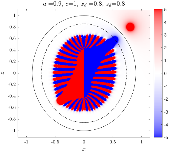
The solution (60) is plotted in Figure 12 for three different aspect ratios. For the low aspect ratios we partially see something like an image point charge at $x\approx x_{h},z\approx z_{h}$ . For higher aspect ratios, we see that the solution does converge down to $x=a^{2}/x_{d}$ as we reasoned is possible for thin spheroids, and certainly one can conclude that the condition for convergence is not $\xi>\xi_{h}$ . For low aspect ratios, $\xi_{i}\rightarrow\xi_{h}$ , which both appear to lie on the extent of the domain of convergence, while for higher aspect ratios, $\xi_{h}$ is way off and $\xi_{i}$ is reasonably close. It also appears that convergence could depend on $\eta$ and $\phi$ , which is possible analytically if $\eta$ and $\phi$ were to change the behavior of the sum over $m$ as $n\rightarrow\infty$ .

Only up to $n,m=85$ could be used in Figure 12 because the factor $(n+m)!$ overflows for any higher $n,m$ . This problem could be avoided by using normalized Legendre functions fukushima2014prolate, which would allow more terms to be included in the series, giving a clearer picture of the boundary between convergence and divergence.

IV Point charge inside spheroid

We now move on to sources placed inside a conducting spheroidal boundary, where the image systems lie outside the spheroid.

IV.1 Point charge at the center

The simplest case is that of a point charge located exactly at the center. The excitation potential is

\displaystyle V_{e}=\frac{f}{r}=\sum_{n=0}^{\infty}(2n+1)P_{n}(0)Q_{n}(\xi)P_{n}(\eta).\qquad

(69)

Note that for $n$ odd, $P_{n}(0)=0$ . The total potential inside is $V=V_{e}+V_{r}$ , where

\displaystyle V_{r}=-\sum_{n=0}^{\infty}(2n+1)\frac{Q_{n}(\xi_{0})}{P_{n}(\xi_{0})}P_{n}(0)P_{n}(\xi)P_{n}(\eta),

(70)

which converges inside a spheroidal volume with surface $\xi_{h}=2\xi_{0}^{2}-1$ . Now we want to determine the form of the image, which must lie outside this spheroid $\xi=\xi_{h}$ . For the similar problem of a charge located inside a cylinder majic2020cylinder, the image lies on the $z=0$ plane with a circular hole. So at least for thin long spheroids we should expect a similar disk image, where the hole touches the spheroid of divergence. So we will assume that the image lies on

\displaystyle\rho\geq\rho_{h}=f\sqrt{\xi_{h}^{2}-1},\quad z=0,

(71)

which is depicted in Figure 13. But before deriving the exact analytic continuation of $V_{r}$ , lets consider some simple approximations.

IV.2 leading order approximation

Here we look for an approximation analogous to that of the point charge approximation for the source outside, by analyzing the limit of the series coefficients as $n\rightarrow\infty$ . In addition to the limits for the Legendre functions in (37), we need the limit for $P_{n}(0)$ :

\displaystyle P_{n}(0)\rightarrow

\displaystyle~\sqrt{\frac{2}{n\pi}}(-)^{n/2}\left[1-\frac{1}{4n}+\mathcal{O}(n^{-2})\right].

(72)

Then as $n\rightarrow\infty$ the coefficients in the series (70) go to leading order as:

\displaystyle\frac{Q_{n}(\xi_{0})}{P_{n}(\xi_{0})}P_{n}(0)\rightarrow\frac{\sqrt{2\pi/n}(-)^{n/2}}{(\xi_{0}+\sqrt{\xi_{0}^{2}-1})^{2n+1}}.

(73)

We want to find a simple function that matches this limit, that when substituted in (70), has a simple closed form for the corresponding series. For the infinite conducting cylinder, the leading order approximation is two point charges offset on the imaginary $z$ -axis at $z=\pm 2i$ majic2020cylinder, which appears in real space as an excavated disk. So for the spheroid, we find that two point charges offset by $z=\pm i\rho_{h}$ is a good approximation. The spheroidal series expansion for this is easily found from the inverse distance expansion Morse1953:

	$\displaystyle V^{(0)}$	$\displaystyle=\frac{if\sqrt{\xi_{h}}}{\sqrt{\rho^{2}+(z-i\rho_{h})^{2}}}-\frac{if\sqrt{\xi_{h}}}{\sqrt{\rho^{2}+(z+i\rho_{h})^{2}}}$
		$\displaystyle=-2i\sqrt{\xi_{h}}\sum_{n=0}^{\infty}(2n+1)Q_{n}(i\rho_{h}/f)P_{n}(\xi)P_{n}(\eta),$		(74)

where we have introduced prefactors so the series coefficients match those in (73) in the limit $n\rightarrow\infty$ . $V^{(0)}$ is a good approximation to $V_{r}$ for fatter spheroids, accurate to within 1% (a constant correction term should be applied to $V^{(0)}$ , replacing the $n=0$ term in (74) with the term in (70)). The approximation works better for rounder spheroids; for $c=2f$ , the approximation is visually indistinguishable from the exact analytic continuation plotted in Figure 14. In fact (74) reduces to the image approximation for the cylinder if we take $c\rightarrow\infty$ with $a$ fixed.

IV.3 First order correction

A first order correction can be found in a similar manner, by considering the next order in the coefficients for the Legendre functions, which allows us to deduce the limit of the coefficients in $V_{r}-V^{(0)}$ :

\displaystyle(2n+1)\bigg[\frac{Q_{n}(\xi_{0})}{P_{n}(\xi_{0})}P_{n}(0)-2i\sqrt{\xi_{h}}Q_{n}(i\rho_{h}/f)\bigg]\rightarrow~\sqrt{\frac{\pi}{2n}}(-)^{n/2}\frac{\xi_{0}^{3}}{\xi_{h}^{3/2}}\frac{\Big(\xi_{0}+\sqrt{\xi_{0}^{2}-1}\Big)^{-2n-1}}{\sqrt{\xi_{0}^{2}-1}}.

(75)

Now consider the limit of

\displaystyle(2n+1)\int Q_{n}(u)\mathrm{d}u~=~Q_{n+1}(u)-Q_{n-1}(u)~\rightarrow~\sqrt{\frac{2\pi}{n}}\frac{(u^{2}-1)^{1/4}}{(u+\sqrt{u^{2}-1})^{n+1/2}},

(76)

which can be matched to the limit of (75) with $u=i\rho_{h}/f$ and the right prefactor. This leads to the first order correction $V^{(1)}$ , writing $V_{r}\approx V^{(0)}+V^{(1)}$ :

\displaystyle V^{(1)}=-\frac{\xi_{0}^{3}}{2\xi_{h}^{3/2}\sqrt{\xi_{0}^{2}-1}}\sum_{n=0}^{\infty}(2n+1)\int^{i\rho_{h}/f}Q_{n}(u)\mathrm{d}u~P_{n}(\xi)P_{n}(\eta).

(77)

(For $n=0$ , $\int^{i\rho_{h}/f}Q_{0}(x)\mathrm{d}x=1-\rho_{h}/f\tan^{-1}(f/\rho_{h})-\log(1+f^{2}/\rho_{h}^{2})/2$ ). The series for $V^{(1)}$ has a simple closed form expression:

\displaystyle V^{(1)}=\frac{\xi_{0}^{3}}{2\xi_{h}^{3/2}\sqrt{\xi_{0}^{2}-1}}\text{Re}\big\{\log\frac{2\rho_{h}}{\rho_{h}-iz+\sqrt{\rho_{h}^{2}-2iz\rho_{h}-r^{2}}}\big\},

(78)

which is also singular on the inverted disk $\rho>\rho_{h}$ , $z=0$ . (78) can be verified by expanding (77) onto spherical harmonics and comparing with the first order correction for the cylinder in majic2020cylinder. $V^{(1)}$ has a positive surface charge density that decreases with $\rho$ .

IV.4 Analytic continuation - image disk

Figure 13: Schematic of the problem of a point charge centered in a prolate spheroid, roughly showing the proposed disk image with singular rings that extends out to infinity. Red represents positive charge and blue negative.

For the 2D problem for a source centered in an ellipse, we discovered that the image system was a series of point charges on the $y$ -axis - the thin axis of the ellipse. An intuitive generalization of this to the prolate spheroid would be a series of rings on the $xy$ -plane over the thin axes of the spheroid. (For an oblate spheroid we might expect the images to lie on the $z$ -axis but that is outside our scope).

To find a mathematical expression for the analytic continuation of $V_{r}$ , we could follow the approach for the infinite cylinder majic2020cylinder and search for an expression as a sum or integral of cylindrical harmonics $J_{0}(k\rho)e^{-k|z|}$ , since this expression should converge everywhere except this image disk. However, there isn’t a clear ansatz for this is – for the cylinder the solution is a discrete sum over $k=k_{n}$ , the $n^{th}$ zeros of $J_{0}$ , but there seems no reason why $V_{r}$ couldn’t be a sum over different values of $k$ , or even an integral over $0\leq k<\infty$ . So instead we will use a different basis that also shares this plane singularity - radially inverted irregular oblate spheroidal harmonics (RIIOSHs). They are singular on the $z=0$ plane and also come with a hole in the middle, which can be fitted to match the assumed image domain (71) exactly. The RIIOSHs are $r^{-1}Q_{n}(i\bar{\chi})P_{n}(\bar{\zeta})$ , where $\hat{\chi},\hat{\zeta}$ are radially inverted oblate spheroidal coordinates:

\displaystyle\hat{\chi}

\displaystyle=\frac{1}{\sqrt{2}\rho_{h}}\sqrt{\hat{r}^{2}-\rho_{h}^{2}+\sqrt{(\hat{r}^{2}-\rho_{h}^{2})^{2}+(2\rho_{h}u\hat{r})^{2}}},\qquad\hat{\zeta}=\frac{u\hat{r}}{\rho_{h}\hat{\chi}},\qquad\hat{r}=\frac{\rho_{h}^{2}}{r}.

(79)

$\rho_{h}$ is the focal disk radius which has been set so that the RIIOSHs are then singular on the domain (71). To expand $V_{r}$ in terms of RIIOSHs, we first expand the prolate spheroidal harmonics in (70) in terms of regular spherical harmonics buchdahl1977relation, and then expand the spherical harmonics in terms of RIIOSHs. The required expansion can be obtained by applying radial inversion to a well known transformation formula between the irregular spherical harmonics and the irregular (external) oblate spheroidal harmonics jeffery1916relations. Inserting these expansions into (70) and rearranging the summation order gives

	$\displaystyle V_{r}=\sum_{k=0:2}^{\infty}\Bigg\{\sum_{p=0:2}^{k}\Bigg[\sum_{n=p:2}^{\infty}(2n+1)\frac{Q_{n}(\xi_{0})}{P_{n}(\xi_{0})}$	$\displaystyle P_{n}(0)\frac{(-)^{\frac{n-p}{2}}(n+p-1)!!}{p!(n-p)!!}\Bigg]$
		$\displaystyle\times\frac{(k+p-1)!!}{p!(k-p)!!}\left(\frac{\rho_{h}}{f}\right)^{k}\Bigg\}~(2k+1)i^{k+1}~\frac{\rho_{h}}{r}Q_{k}(i\hat{\chi})P_{k}(\hat{\zeta}).$		(80)

The series over $n$ appears to converge quickly and be numerically stable (checked for $p\leq 100$ ). But the sum over $p$ suffers from catastrophic cancellation like in (53) - the terms are only accurate for $k\lesssim 44$ . Still, (80) offers a significant analytic continuation of the original series (70).

We can also improve the rate of convergence of (80) by adding and subtracting the two forms for $V^{(0)}$ in (74):

$\displaystyle V_{r}=\frac{ic\sqrt{\xi_{h}}}{\sqrt{\rho^{2}+(z-i\rho_{h})^{2}}}$	$\displaystyle-\frac{ic\sqrt{\xi_{h}}}{\sqrt{\rho^{2}+(z+i\rho_{h})^{2}}}$
$\displaystyle-\sum_{k=0:2}^{\infty}\Bigg\{$	$\displaystyle\sum_{p=0:2}^{k}\Bigg[\sum_{n=p:2}^{\infty}(2n+1)\bigg(\frac{Q_{n}(\xi_{0})}{P_{n}(\xi_{0})}P_{n}(0)-2i\sqrt{\xi_{h}}Q_{n}(i\rho_{h}/f)\bigg)$
	$\displaystyle\times\frac{(-)^{\frac{n-p}{2}}(n+p-1)!!}{p!(n-p)!!}\Bigg]\frac{(k+p-1)!!}{p!(k-p)!!}\left(\frac{\rho_{h}}{f}\right)^{p}\Bigg\}~(2k+1)i^{k+1}~\frac{\rho_{h}}{r}Q_{k}(i\hat{\chi})P_{k}(\hat{\zeta}).$	(81)

The faster convergence means (81) can accurately compute $V_{r}$ in a larger domain relative to (80) before numerical cancellations become a problem. Eq. (81) is plotted in Figure 14 for spheroids of different aspect ratios. Numerical errors are high where $\hat{\chi}$ is small, near the image disk, but we can still make loose deductions of image charge density from the plots. $V_{r}$ changes sign as it moves out in the $\rho$ direction, indicating that the image disk charges also change sign in this way. A similar pattern is seen for the infinite cylinder, but there the image changes sign at regularly spaced intervals, while the pattern here appears to stretch as $\rho$ increases. In the cylinder the surface charge density also became infinite at these evenly spaced intervals to make singular rings, so we might expect these to occur for the spheroid (and there is at least one singular ring at $\xi_{h}$ ). From the 2D problem of a source centered in an ellipse, we could guess that the image rings would lie at $\text{acosh}\xi=2k\text{acosh}\xi_{0}$ (and $\eta=0$ ) – at least the first image ring at $\text{acosh}\xi_{h}=2\text{acosh}\xi_{0}$ agrees with this hypothesis.

Unfortunately like in Section III.4, subtracting $V^{(1)}$ does not make the RIIOSH series converge faster, although $V^{(0)}+V^{(1)}$ does match the analytic continuation well for the inner part of the image disk.

In order to prove that the image lies completely on the $z=0$ plane, we would have to show that the coefficients in either series (80) or (81) grow at less than an exponential rate as $k\rightarrow\infty$ so that the $Q_{k}(i\hat{\chi})$ will make the series converge. This does appear to be true numerically for the values of $k$ we can compute without catastrophic cancellation.

IV.5 Point charge off axis inside spheroid

We can extend some of the concepts of the previous sections to offset charges. For the ellipse, the images were point sources on a hyperbola, so we might expect that the images for the spheroid would lie on the hyperboloid $\eta=\eta_{d}$ . But in this section we only manage to find an approximate image ring. Let the source charge lie at $x=x_{d}>0,~y=0,~z=z_{d}>0$ , or equivalently at $\eta=\eta_{d}>0,~\xi=\xi_{d},~\phi=0$ . The excitation potential is

\displaystyle V_{e}=\frac{f}{\sqrt{(x-x_{d})^{2}+y^{2}+(z-z_{d})^{2}}},

(82)

and the reflected potential is

\displaystyle V_{r}=-\sum_{n=0}^{\infty}\sum_{m=-n}^{n}(-)^{m}\frac{(n-m)!^{2}}{(n+m)!^{2}}\frac{Q_{n}^{m}(\xi_{0})}{P_{n}^{m}(\xi_{0})}P_{n}^{m}(\xi_{d})P_{n}^{m}(\eta_{d})P_{n}^{m}(\xi)P_{n}^{m}(\eta)\cos m\phi.

(83)

Like for the off-axis external source in Section III.5, the exact rate of convergence depends on the values of the whole sum over $m$ as $n\rightarrow\infty$ , but this is not straightforward to determine analytically. Instead we will use a crude analysis by considering the limit as $n\rightarrow\infty$ for single terms with fixed $m$ . In this case the series over $n$ diverges outside the external spheroid $\xi_{h}=(2\xi_{0}^{2}-1)\xi_{d}-2\xi_{0}\sqrt{\xi_{0}^{2}-1}\sqrt{\xi_{d}^{2}-1}$ , or $\text{acosh}\xi_{h}=2\text{acosh}\xi_{0}-\text{acosh}\xi_{d}$ . In contrast to the case of an external off axis source, $\xi_{h}$ appears to closely fit the boundary of divergence of the series (83), from numerical tests across a wide range of aspect ratios and source positions.

Next we investigate two ways to approximate the terms in this sum as $n\rightarrow\infty$ for $m$ fixed, which work better for different locations of the source.

IV.5.1 Point charge near surface

When the source charge is near the surface, we use an approximation of a point charge somewhat opposite the source charge. In the series (83), we replace the coefficients with

\displaystyle-\frac{Q_{n}^{m}(\xi_{0})}{P_{n}^{m}(\xi_{0})}P_{n}^{m}(\xi_{d})\rightarrow q_{h}Q_{n}^{m}(\xi_{h})\big[1+\mathcal{O}(1/n)\big],

(84)

where $q_{h}=-((\xi_{h}^{2}-1)/(\xi_{d}^{2}-1))^{1/4}$ is the strength of the image charge. Substituting this approximation into (83) gives an approximate image potential $\dot{V}_{r}^{0}$ :

	$\displaystyle\dot{V}_{r}^{0}$	$\displaystyle=q_{h}\sum_{n=0}^{\infty}\sum_{m=-n}^{n}\frac{(n-m)!^{2}}{(n+m)!^{2}}(-)^{m}Q_{n}^{m}(\xi_{h})P_{n}^{m}(\eta_{d})P_{n}^{m}(\xi)P_{n}^{m}(\eta)\cos m\phi$
		$\displaystyle=\frac{q_{h}f}{\sqrt{(x-x_{h})^{2}+y^{2}+(z-z_{h})^{2}}}$		(85)

where $x_{h}=f\sqrt{\xi_{h}^{2}-1}\sqrt{1-\eta_{d}^{2}},~z_{h}=f\xi_{h}\eta_{d}$ . We can then express the exact potential $V_{r}$ as a faster converging series by adding and subtracting the different forms of $\dot{V}_{r}^{0}$ :

	$\displaystyle V_{r}=$	$\displaystyle\frac{fq_{h}}{\sqrt{(x-x_{h})^{2}+y^{2}+(z-z_{h})^{2}}}$
		$\displaystyle-\sum_{n=0}^{\infty}\sum_{m=-n}^{n}\frac{(n-m)!^{2}}{(n+m)!^{2}}(-)^{m}(2n+1)\bigg(\frac{Q_{n}^{m}(\xi_{0})}{P_{n}^{m}(\xi_{0})}P_{n}^{m}(\xi_{d})+q_{h}Q_{n}^{m}(\xi_{h})\bigg)P_{n}^{m}(\eta_{d})P_{n}^{m}(\xi)P_{n}^{m}(\eta)\cos m\phi.$		(86)

But (85) fails when the source charge is near the focus of the spheroid, since the problem becomes more rotationally symmetric, and a single image point charge placed off axis will break the symmetry.

IV.5.2 Point charge near focus

In this case we look to an approximation that is a generalization of the ring image (74) for the source at the center. The coefficients in (83) can instead be approximated as

\displaystyle-\frac{Q_{n}^{m}(\xi_{0})}{P_{n}^{m}(\xi_{0})}P_{n}^{m}(\eta_{d})\rightarrow q_{r}Q_{n}^{m}(\xi_{r})\big[1+\mathcal{O}(1/n)\big],

(87)

where we use new coordinates with subscript _r for “ring”, with $\xi_{r}=(2\xi_{0}^{2}-1)\eta_{d}-2\xi_{0}\sqrt{\xi_{0}^{2}-1}\sqrt{\eta_{d}^{2}-1}$ and $q_{r}=-\text{abs}\{((\xi_{r}^{2}-1)/(\eta_{d}^{2}-1))^{1/4}\}$ , which are similar to the definitions of $\xi_{h}$ and $q_{h}$ , but with $\xi_{d}\leftrightarrow\eta_{d}$ . Substituting the approximation (87) into (83) gives an approximate image potential $\mathring{V}_{r}^{0}$ :

	$\displaystyle\mathring{V}_{r}^{0}$	$\displaystyle=2q_{r}\sum_{n=0}^{\infty}\sum_{m=-n}^{n}\frac{(n-m)!^{2}}{(n+m)!^{2}}(2n+1)~\mathrm{Re}\{i^{m-1}Q_{n}^{m}(\xi_{r})\}P_{n}^{m}(\xi_{d})~P_{n}^{m}(\xi)P_{n}^{m}(\eta)\cos m\phi$
		$\displaystyle=\text{sign}\bigg(\frac{z-\mathrm{Re}\{z_{r}\}}{\mathrm{Im}\{x_{r}\}}-\frac{x+\mathrm{Re}\{x_{r}\}}{\mathrm{Im}\{z_{r}\}}\bigg)\mathrm{Re}\bigg\{\frac{-2ifq_{r}}{\sqrt{(x-x_{r})^{2}+y^{2}+(z-z_{r})^{2}}}\bigg\}$		(88)

where $x_{r}=-f\sqrt{\xi_{r}^{2}-1}\sqrt{\xi_{d}^{2}-1},~z_{r}=f\xi_{r}\xi_{d}$ . Notice $\xi_{d}$ behaves as the $\eta$ coordinate of the image charge, and $\xi_{d}>1$ outside the usual range of $\eta$ , while $\xi_{r}$ is complex. This results in $x_{r}$ and $z_{r}$ both being complex. The projection of the image onto real space is a ring similar to (74) but offset in the $x$ and $z$ directions, and tilted, such that the ring lies on the hyperbolic surface $\eta=\eta_{d}$ , and at closest approach to the spheroid surface, the ring passes through the real image point charge (85). The sign function makes the potential continuous through the hole in the ring. When the source is located at the center, (88) coincides with (74).
We can then express the exact potential $V_{r}$ as a faster converging series by adding and subtracting the different forms of $\mathring{V}_{r}^{0}$ :

$\displaystyle V_{r}=$	$\displaystyle\text{sign}\bigg(\frac{z-\mathrm{Re}\{z_{r}\}}{\mathrm{Im}\{z_{r}\}}-\frac{x+\mathrm{Re}\{x_{r}\}}{\mathrm{Im}\{x_{r}\}}\bigg)\mathrm{Re}\bigg\{\frac{-2ifq_{r}}{\sqrt{(x-x_{r})^{2}+y^{2}+(z-z_{r})^{2}}}\bigg\}$
	$\displaystyle-\sum_{n=0}^{\infty}\sum_{m=-n}^{n}\frac{(n-m)!^{2}}{(n+m)!^{2}}(2n+1)\bigg((-)^{m}\frac{Q_{n}^{m}(\xi_{0})}{P_{n}^{m}(\xi_{0})}P_{n}^{m}(\eta_{d})+2q_{r}\mathrm{Re}\{i^{m-1}Q_{n}^{m}(\xi_{r})\}\bigg)$
	$\displaystyle\hskip 199.16928pt\times P_{n}^{m}(\xi_{d})P_{n}^{m}(\xi)P_{n}^{m}(\eta)\cos m\phi.$	(89)

The approximations (84) and (87) apply only for $n\gg|m|$ , although $m$ ranges from $-\infty$ to $\infty$ . One way to quantify the rate of convergence of the double series numerically is to sum over $m$ first and then treat it as a single series over $n$ . In this respect, (86) and (89) improve the rate of convergence of the series a similar amount to that of the series (46) for the point charge outside the spheroid, i.e. the terms converge faster by a factor of $n$ . The approximations are shown in Figure 15 for a point charge near the surface and near the axis, and roughly satisfy the boundary condition $V=0$ on the spheroid surface (their accuracy can be improved by a correction of the constant $n=0$ term). In terms of determining the analytic continuation of $V_{r}$ , both $\dot{V}_{r}^{0}$ and $\mathring{V}_{r}^{0}$ exhibit a singular point at $\xi=\xi_{h},\eta=\eta_{d},\phi=0$ , and this singularity is also partially visible in plots of the exact potential $V_{r}$ (partially due to the boundary of the domain of convergence $\xi=\xi_{h}$ ). $\mathring{V}_{r}^{0}$ is also singular on the exterior disk that lies co-planar with the ring, but the exact analytic continuation of $V_{r}$ is not necessarily singular there.

We can even combine the point image and ring image approximations to increase their accuracy. By adding the two and weighting them according to how close the source is to the surface, the coefficients can be much more closely matched, and we can create a universal approximation for any source position (except the focal points – see section IV.7). A simple weighting may be

\displaystyle\dot{\mathring{V}}_{r}^{0}=\sqrt{\frac{\xi_{d}^{2}-1}{\xi_{0}^{2}-1}}\dot{V}_{r}^{0}+\left(1-\sqrt{\frac{\xi_{d}^{2}-1}{\xi_{0}^{2}-1}}\right)\mathring{V}_{r}^{0}.

(90)

The weighting factor $\sqrt{\xi_{d}^{2}-1}/\sqrt{\xi_{0}^{2}-1}$ is chosen so that near the surface $\xi_{d}\rightarrow\xi_{0}$ leaving $\dot{\mathring{V}}_{r}^{0}\rightarrow\dot{V}_{r}^{0}$ , while near the focus $\xi_{d}\rightarrow 1$ leaving $\dot{\mathring{V}}_{r}^{0}\rightarrow\mathring{V}_{r}^{0}$ . This approximation is more accurate than $\dot{V}_{0}^{r}$ or $\mathring{V}_{0}^{r}$ separately, but there may be a more optimal weighting.

IV.6 Point charge on axis near the tip

If the source charge is located on the $z$ -axis with $z>f$ , we have $\eta_{d}=1$ . Here the ring approximation $\mathring{V}_{r}^{0}$ fails and the point charge approximation $\dot{V}_{r}^{0}$ reduces to a point charge on the axis. The series solution with improved rate of convergence (63) reduces to

\displaystyle V_{r}=

\displaystyle\frac{fq_{h}}{\sqrt{\rho^{2}+(z-h)^{2}}}-\sum_{n=0}^{\infty}(2n+1)\bigg(\frac{Q_{n}(\xi_{0})}{P_{n}(\xi_{0})}P_{n}(\xi_{d})+q_{h}Q_{n}(\xi_{h})\bigg)P_{n}(\xi)P_{n}(\eta).

(91)

where $h=f\xi_{h}$ . We can attempt to analytically continue this by assuming that $V_{r}$ is singular on the $z$ axis for $z\geq h$ . We follow a similar analysis to that done for the point charge on the axis outside the spheroid or in the center, that is, expand the potential on a basis of harmonic functions that share the same singularity as the reflected potential. In this case we use “radially inverted irregular offset prolate spheroidal harmonics”, or RIIOPSHs, which are also singular on the $z$ -axis from $z=h$ to infinity. Skipping the details, we can expand the series (86) in terms of regular spherical harmonics centered at the origin using the relationships between spheroidal and spherical harmonics (equation (2.21) of majic2016thesis), then define a radially inverted radius $\hat{r}=h^{2}/r$ and treat this as the new radius, and expand these spherical harmonics onto offset irregular spheroidal harmonics (Eq. 2.28 of majic2016thesis). The result is

	$\displaystyle V_{r}=\frac{fq_{h}}{\sqrt{\rho^{2}+(z-h)^{2}}}-\sum_{k=0}^{\infty}(2k+1)$	$\displaystyle\sum_{p=0}^{k}\frac{(k+p)!}{p!^{2}(k-p)!}\sum_{n=p:2}^{\infty}(-)^{(n+p)/2+k}\frac{(n+p-1)!!}{p!(n-p)!!}\left(\frac{h}{f}\right)^{p+1}$
		$\displaystyle\times(2n+1)\left(\frac{Q_{n}(\xi_{0})}{P_{n}(\xi_{0})}P_{n}(\xi_{d})+q_{h}Q_{n}(\xi_{h})\right)~\frac{f}{r}Q_{k}(\hat{\xi})P_{k}(\hat{\eta})$		(92)

where $\hat{\xi}=\xi(r\rightarrow\hat{r}),~\hat{\eta}=\eta(r\rightarrow\hat{r})$ . This series provides at least a significant analytic continuation of the potential $V_{r}$ , as shown in Figure 16. The boundary of the domain of convergence of the RIIOPSH series is a coordinate of constant $\hat{\xi}$ , which is a dimpled sphere where the dimple cuts into the sphere on the $z$ -axis for $z>h$ . Like the series (53), the series (92) suffers from numerical problems which are apparent near the singularity, prohibiting us from seeing the image charge distribution in detail. But the RIIOPSH series still provides a significant analytic continuation of the potential, and shows us where the singularities $aren^{\prime}t$ – the continuation (92) can also be evaluated for large negative $z$ values and large $x$ values, and plots including these regions suggest that the singularity is concentrated to the $z$ -axis for $z>h$ . From the analogous problem for the ellipse (see Fig. 7), we could also guess that image contains singular points on the $z$ -axis at $z=f\cosh(2k\text{acosh}\xi_{0}\pm\xi_{d})$ for $k=1,2,3...$ .

IV.7 Point charge on focal point

For a source charge on the top focal point, i.e. $\xi_{d}=1,~\eta_{d}=1,~z_{d}=f$ , both approximations (85) and (88) fail due to the factor $(\xi_{d}^{2}-1)^{-1/4}$ in $q_{h}$ and $(\eta_{d}^{2}-1)^{-1/4}$ in $q_{r}$ . Here the spheroidal harmonic solution is

\displaystyle V_{r}^{f}=-\sum_{n=0}^{\infty}(2n+1)\frac{Q_{n}(\xi_{0})}{P_{n}(\xi_{0})}P_{n}(\xi)P_{n}(\xi).

(93)

The coefficients for $n\rightarrow\infty$ go as

\displaystyle\frac{Q_{n}(\xi_{0})}{P_{n}(\xi_{0})}\rightarrow\pi\bigg(\xi_{0}+\sqrt{\xi_{0}^{2}-1}\bigg)^{-2n-1}\big[1+\mathcal{O}(1/n)\big],

(94)

but unlike in the previous sections we cannot easily match this behavior simply with one or two Legendre functions in the numerator because for $n\rightarrow\infty$ , both $P_{n}$ and $Q_{n}$ have a factor of $n^{-1/2}$ which is not present in (94). Instead we find that a good approximation involves the fractional order Legendre function $Q_{n}^{1/2}$ which does not have this $n^{-1/2}$ dependence. The approximate potential is that of a fractional multipole of degree 1/2, or a “ $\sqrt{2}$ -pole”, which in a sense is half way between a monopole and a dipole. The theory of fractional multipoles and how to create them using fractional derivatives is investigated in engheta1996fractional. They define in their equation (30) the multipole of degree $\alpha$ by applying the fractional derivative ${}_{-\infty}\!D_{z}^{\alpha}$ to a monopole at the origin (where $-\infty$ is a lower value like that used in integration, $z$ is the variable to be differentiated, and $\alpha$ is the order of differentiation). For $\alpha=1/2$ , with our normalization, this is

$\displaystyle V_{\sqrt{2}}$	$\displaystyle=_{-\infty}\!D^{1/2}_{z}\frac{\ell^{1/2}}{\sqrt{\rho^{2}+z^{2}}}$	(95)
	$\displaystyle=\frac{\ell^{1/2}}{\Gamma(1/2)}\frac{\partial}{\partial z}\int_{0}^{\infty}\frac{v^{-1/2}}{\sqrt{\rho^{2}+(z-v)^{2}}}\mathrm{d}v$	(96)
	$\displaystyle=\frac{\ell^{1/2}\Gamma(3/2)}{r^{3/2}}P_{1/2}(-\cos\theta).$	(97)

where $\ell$ is an arbitrary length. $V_{\sqrt{2}}$ is a solution to Laplace’s equation except on the positive $z$ -axis due to the Legendre function $P_{1/2}$ being singular at $\cos\theta=1$ . The line charge density of this multipole is $-z^{-3/2}$ for $z>0$ , plus a positive point charge at the origin. What we want for an approximate image is $V_{\sqrt{2}}$ but translated up the $z$ -axis, so that the singularity extends upwards from the height where the series (93) diverges, that is $\rho=0,z=h$ , where $h=\xi_{h}f$ and $\xi_{h}=2\xi_{0}^{2}-1$ . We shall call this approximation $V_{\sqrt{2}}^{h}$ . It turns out that the coefficients of the spheroidal harmonic expansion of this image have exactly the behavior of the coefficients in (94). In order to derive these coefficients we begin with the known expansion of the monopole:

\displaystyle V_{1}^{h}=\frac{f}{\sqrt{\rho^{2}+(z-h)^{2}}}=\sum_{n=0}^{\infty}(2n+1)Q_{n}(\xi_{h})P_{n}(\xi)P_{n}(\eta),

(98)

and note that the symmetry about $z\leftrightarrow h$ means that we can derive the $\sqrt{2}$ -pole by differentiating the monopole with respect to $h$ instead of $z$ . Applying this to the expansion (98) and modifying the prefactors so that the series coefficients match those in (94) leads to

	$\displaystyle V_{\sqrt{2}}^{h}=$	$\displaystyle-\sqrt{2\pi f(\xi_{h}^{2}-1)}~~_{-\infty}\!D_{h}^{1/2}V_{1}^{h}$
	$\displaystyle=$	$\displaystyle-\sqrt{2\pi f(\xi_{h}^{2}-1)}\sum_{n=0}^{\infty}(2n+1)~_{-\infty}\!D_{h}^{1/2}\big[Q_{n}(\xi_{h})\big]P_{n}(\xi)P_{n}(\eta).$		(99)

The fractional derivative of $Q_{n}(\xi_{h})$ can be evaluated using formula 7.133 from tables2014, which gives the result in terms of a Legendre function of order $m=1/2$ :

\displaystyle V_{\sqrt{2}}^{h}=-\sqrt{2\pi}(\xi_{h}^{2}-1)^{1/4}\sum_{n=0}^{\infty}(2n+1)Q_{n}^{1/2}(\xi_{h})P_{n}(\xi)P_{n}(\eta),

(100)

Conveniently, the Legendre function $Q_{n}^{1/2}$ has a simple formula:

\displaystyle Q_{n}^{1/2}(\xi_{h})=\frac{\sqrt{\pi/2}}{(\xi_{h}^{2}-1)^{1/4}}\left(\xi_{h}+\sqrt{\xi_{h}^{2}-1}\right)^{-n-1/2}.

(101)

The closed form expression of $V_{\sqrt{2}}$ is

\displaystyle V_{\sqrt{2}}^{h}=-\frac{\pi}{\sqrt{2}}\frac{\sqrt{\xi_{h}^{2}-1}f^{3/2}}{(\rho^{2}+(z-h)^{2})^{3/2}}P_{1/2}(-\cos\theta_{h}),

(102)

where $\cos\theta_{h}=(z-h)/\sqrt{\rho^{2}+(z-h)^{2}}$ , and the Legendre function $P_{1/2}$ can be evaluated via its hyper-geometric series. The approximate solution $V_{e}+V_{\sqrt{2}}^{h}$ is plotted in Fig. 17, showing a negative image point charge at $z=h$ and a positive line charge distribution for $z>h$ , decaying as $z$ increases. How similar is the singularity of the exact solution?

We can guess that the potential is singular on the $z$ axis for $z\geq h$ , and obtain its analytic continuation following a similar analysis to that done for the point charge on the axis for $z>f$ , but starting with the series (93) (also to minimize numerical cancellations we add (102) and subtract (100)). The result is

	$\displaystyle V_{r}^{f}=V_{\sqrt{2}}^{h}-\sum_{k=0}^{\infty}(2k+1)$	$\displaystyle\sum_{p=0}^{k}\frac{(k+p)!}{p!^{2}(k-p)!}\sum_{n=p:2}^{\infty}(-)^{(n+p)/2+k}\frac{(n+p-1)!!}{p!(n-p)!!}\left(\frac{h}{f}\right)^{p+1}$
		$\displaystyle\times(2n+1)\left(\frac{Q_{n}(\xi_{0})}{P_{n}(\xi_{0})}-\sqrt{2\pi}(\xi_{h}^{2}-1)^{1/4}Q_{n}^{1/2}(\xi_{h})\right)\frac{f}{r}Q_{k}(\hat{\xi})P_{k}(\hat{\eta}).$		(103)

Like series (92), this suffers from numerical problems for $k\gtrsim 20$ , and is plotted in Figure 17 (right) with as much accuracy as possible. It appears that the approximation $V_{\sqrt{2}}^{h}$ closely matches the singularity of $V_{r}$ near $z\approx h$ . The main visible difference between the images of a point charge on the focal point $z_{d}=f$ or above the focus $f<z_{d}<c$ , is that for $z_{d}=f$ the image line charge density is positive for $z\gtrsim h$ , but for $z_{d}>f$ the image line charge is negative for $z\gtrsim h$ , then becomes positive higher up the axis. From the analogous problem for the ellipse, we could also guess that image contains singular points on the $z$ -axis at $z=f\cosh(2k\text{acosh}\xi_{0})$ for $k=1,2,3...$ . It is interesting to note that the innermost point of the image at $z=h$ is the same as the critical distance $d_{c}$ (Eq. (39)) for the source charge located outside the spheroid on the axis. For a source at $z_{d}=d_{c}$ , the approximate point image (44) lies exactly on the focal point.

V Conclusion

We have investigated obtaining reduced images of point sources inside or outside ellipses and prolate spheroids, manipulating the series solutions to reveal the singularities of the reflected potential, and deriving approximate images that mimic these singularities. For the ellipse, simple reduced images could be found for every position of the source. For an exterior source the problem was solved via series sten1996focal and reflection alshal2021image, and both could provide analytic continuation of the potential to reveal the image on the focal line, plus a point image if the source was close. For an internal source, we derived a solution as a series of image charges lying on a hyperbola.

For a point charge on the axis of a prolate spheroid, within the critical distance to the surface, numerical analysis of a series of stretched spheroidal harmonics (53) suggests that the reduced image lies on the segment extending from the lower focus up to the image point: $-f<z<h$ , and that the top point of the singularity is well matched by the point charge approximation of lindell2001electrostatic. For a point charge off the axis, we have generalized this point charge approximation with the requirement that the coefficients of its series expression have the same asymptotic form as those for the reflected potential.

For a point charge inside the spheroid, we find various image approximations. For a point charge at the center of a prolate spheroid, we also analytically continued the potential using a series of radially inverted oblate spheroidal harmonics, which suggests that the exact image lies on the external disk $z=0$ , $\rho\geq h$ . A similar analysis for the source charge on the axis above the focus was carried out using radially inverted offset prolate spheroidal harmonics which suggests the exact image lies on the $z$ -axis for $z>h$ . For the source charge near the surface, an image point charge opposite the surface is approximately valid. For the source charge near the focal segment, a point charge in complex space or equivalently an image ring/exterior disk is appropriate. For the source exactly on one of the focal points, the image approximation is found to be a $\sqrt{2}$ -pole consisting of a line charge extending up the $z$ -axis.

Acknowledgements.

I wish to thank Victoria University for funding this research via a doctoral scholarship, and an anonymous reviewer for many helpful suggestions.

References

(1) J. C.-E. Sten and I. V. Lindell, “An electrostatic image solution for the conducting prolate spheroid,” Journal of electromagnetic waves and applications, vol. 9, no. 4, pp. 599–609, 1995.
(2) J.-E. Sten, “Focal image charge singularities for the dielectric elliptic cylinder,” Electrical Engineering, vol. 79, no. 1, pp. 9–15, 1996.
(3) I. Lindell, G. Dassios, and K. Nikoskinen, “Electrostatic image theory for the conducting prolate spheroid,” Journal of Physics D: Applied Physics, vol. 34, no. 15, p. 2302, 2001.
(4) I. Lindell and K. Nikoskinen, “Electrostatic Image Theory for the Dielectric Prolate Spheroid,” Journal of Electromagnetic Waves and Applications, vol. 15, no. 8, pp. 1075–1096, 2001.
(5) G. Dassios and J. C.-E. Sten, “The image system and green’s function for the ellipsoid,” Contemporary Mathematics, vol. 494, 2009.
(6) C. Xue and S. Deng, “Green’s function and image system for the Laplace operator in the prolate spheroidal geometry,” AIP Advances, vol. 7, no. 1, p. 015024, 2017.
(7) G. Dassios and J. C.-E. Sten, “On the neumann function and the method of images in spherical and ellipsoidal geometry,” Mathematical Methods in the Applied Sciences, vol. 35, no. 4, pp. 482–496, 2012.
(8) C. Xue, R. Edmiston, and S. Deng, “Image theory for neumann functions in the prolate spheroidal geometry,” Advances in Mathematical Physics, vol. 2018, 2018.
(9) H. Alshal, T. Curtright, and S. Subedi, “Image charges re-imagined,” arXiv preprint arXiv:1808.08300, 2018.
(10) D. Khavinson and E. Lundberg, “The search for singularities of solutions to the dirichlet problem: recent developments,” in CRM Proceedings and Lecture Notes, vol. 51, pp. 121–132, 2010.
(11) S. R. Bell, P. Ebenfelt, D. Khavinson, and H. S. Shapiro, “On the classical dirichlet problem in the plane with rational data,” Journal d’Analyse Mathematique, vol. 100, no. 1, pp. 157–190, 2006.
(12) H. Alshal, T. Curtright, and S. Subedi, “Image charges re-imagined,” Bulgarian Journal of Physics, vol. 48, pp. 202–224, 2021.
(13) T. Curtright, H. Alshal, P. Baral, S. Huang, J. Liu, K. Tamang, X. Zhang, and Y. Zhang, “The conducting ring viewed as a wormhole,” European Journal of Physics, vol. 40, no. 1, p. 015206, 2018.
(14) “NIST Digital Library of Mathematical Functions.” http://dlmf.nist.gov/, Release 1.0.16 of 2017-09-18. F. W. J. Olver, A. B. Olde Daalhuis, D. W. Lozier, B. I. Schneider, R. F. Boisvert, C. W. Clark, B. R. Miller and B. V. Saunders, eds.
(15) G. Nemes and A. B. Olde Daalhuis, “Large-parameter asymptotic expansions for the legendre and allied functions,” SIAM Journal on Mathematical Analysis, vol. 52, no. 1, pp. 437–470, 2020.
(16) T. Havelock, “The moment on a submerged solid of revolution moving horizontally,” Quart. J. Mech. Appl. Math., vol. 5, no. 2, pp. 129–136, 1952.
(17) J. Lebl, Tasty Bits of Several Complex Variables. Lulu. com, 2019.
(18) M. Majic, “New relationships between spherical and spheroidal harmonics and applications,” Master’s thesis, Victoria University of Wellington, 2016.
(19) M. Majic, B. Auguié, and E. C. Le Ru, “Laplace’s equation for a point source near a sphere: improved internal solution using spheroidal harmonics,” IMA Journal of Applied Mathematics, vol. 83, no. 6, pp. 895–907, 2018.
(20) M. Majic, B. Auguié, and E. C. Le Ru, “Spheroidal harmonic expansions for the solution of Laplace’s equation for a point source near a sphere,” Phys. Rev. E, vol. 95, no. 3, 2017.
(21) M. Majic, “Images of point charges in conducting ellipses and prolate spheroids,” Journal of Mathematical Physics, vol. 62, no. 9, p. 092902, 2021.
(22) T. Fukushima, “Prolate spheroidal harmonic expansion of gravitational field,” The Astronomical Journal, vol. 147, no. 6, p. 152, 2014.
(23) M. Majic, “The image of a point charge in an infinite conducting cylinder,” arXiv preprint arXiv:2001.10651, 2020.
(24) P. M. Morse and H. Feshbach, Methods of theoretical physics. New York: McGraw-Hill, 1953.
(25) H. Buchdahl, N. Buchdahl, and P. Stiles, “On a relation between spherical and spheroidal harmonics,” Journal of Physics A: Mathematical and General, vol. 10, no. 11, p. 1833, 1977.
(26) G. B. Jeffery, “The relations between spherical, cylindrical, and spheroidal harmonics,” Proceedings of the London Mathematical Society, vol. s2-16, no. 1, pp. 133–139, 1916.
(27) N. Engheta, “On fractional calculus and fractional multipoles in electromagnetism,” IEEE Transactions on Antennas and Propagation, vol. 44, no. 4, pp. 554–566, 1996.
(28) I. S. Gradshteyn and I. M. Ryzhik, Table of integrals, series, and products. Academic press, 2014.