Cost-effective search for lower-error region in
material parameter space using multifidelity
Gaussian process modeling

Let $r_{\rm expt}$ be the aspect ratio of the precipitate obtained from an experimental image, and $r^{(m)}_{\boldsymbol{x}_{i},{\rm comput}}$ be the aspect ratio predicted using a computational model with the material parameter $\boldsymbol{x}_{i}\in\mathbb{R}^{d}$ and the fidelity level $m\in\{1,\ldots,M\}$. We assumed a set of $N$ candidates $\{\boldsymbol{x}_{i}\}_{i=1}^{N}$ in the material parameter space (for example, grid points uniformly taken in the space). If the higher-fidelity level $m$ is calculated, more accurate results can be obtained though it requires a higher computational cost. Let $\lambda^{(1)}\leq\lambda^{(2)}\leq\ldots\leq\lambda^{(M)}$ be the sampling cost of each fidelity (computational time of the model). The discrepancy between the aspect ratios obtained from the experimental image and through the computational model is defined by

where $t$ is the time and ${\cal T}$ is a set of times when the shapes of precipitates are experimentally measured.

Suppose that the observed discrepancy contains an independent additive noise term given as follows: $y^{(m)}_{\boldsymbol{x}}=f^{(m)}_{\boldsymbol{x}}+\epsilon$, where $\epsilon\sim\mathcal{N}(0,\sigma_{\rm noise}^{2})$. Then, the LER, in which the true discrepancy of the highest-fidelity function $f^{(M)}_{\boldsymbol{x}}$ is less than a given threshold $h$, is defined as

If a large set of the highest-fidelity values of $y_{\boldsymbol{x}_{i}}^{(M)}$ can be obtained for a variety of $\boldsymbol{x}_{i}$, LER can be identified accurately. However, this leads to prohibitive computational costs because the fidelity level $M$ needs the highest computational cost, and further, the number of candidate material parameters is often high. Our goal is to identify the LER with the small total sampling cost (the sum of $\lambda^{(m)}$ over the sampled points).

Suppose we already have the dataset ${\cal D}_{n}=\{(\boldsymbol{x}_{i},y^{(m_{i})}_{\boldsymbol{x}_{i}},m_{i})\}_{i=1}^{n}$ containing a set of triplets consisting of an input $\boldsymbol{x}_{i}\in\mathbb{R}^{d}$, fidelity $m_{i}\in\{1,\ldots,M\}$ and output $y^{(m_{i})}_{\boldsymbol{x}_{i}}\in\mathbb{R}$. To jointly model different fidelity observations with the GP, we used a multifidelity extension of GP regression (MF-GP) [38], which is also known as a co-kriging model. Let $f^{(M)}\sim GP(0,k_{M}(\boldsymbol{x},\boldsymbol{x}^{\prime}))$ be the GP for the highest fidelity $m=M$, in which the prior mean is $0$ and the covariance function is $k_{M}:\mathbb{R}^{d}\times\mathbb{R}^{d}\rightarrow\mathbb{R}$ (the covariance function is also called kernel function). Note that we can set the prior mean as $0$ without loss of generality. We define the output for the lower fidelity $m=M-1,\ldots,1$ recursively from $M$ as follows;

where $g^{(m+1)}\sim GP(0,k_{g}(\boldsymbol{x},\boldsymbol{x}^{\prime}))$ with the kernel function $k_{g}:\mathbb{R}^{d}\times\mathbb{R}^{d}\rightarrow\mathbb{R}$. The function $g^{(m+1)}_{\boldsymbol{x}}$ represents difference between $f^{(m)}_{\boldsymbol{x}}$ and $f^{(m+1)}_{\boldsymbol{x}}$. For example, when $M=3$, we obtain $f^{(2)}_{\boldsymbol{x}}=f^{(3)}_{\boldsymbol{x}}+g^{(3)}_{\boldsymbol{x}}$, and $f^{(1)}_{\boldsymbol{x}}=f^{(2)}_{\boldsymbol{x}}+g^{(2)}_{\boldsymbol{x}}=f^{(3)}_{\boldsymbol{x}}+g^{(3)}_{\boldsymbol{x}}+g^{(2)}_{\boldsymbol{x}}$. The difference between $f^{(3)}_{\boldsymbol{x}}$ and $f^{(2)}_{\boldsymbol{x}}$, which have neighboring fidelity levels, is modeled using the single GP model $g^{(3)}_{\boldsymbol{x}}$. In contrast, the difference between $f^{(3)}_{\boldsymbol{x}}$ and $f^{(1)}_{\boldsymbol{x}}$, whose fidelity levels are more distant from each other, is modeled by the sum of the two GP models $g^{(3)}_{\boldsymbol{x}}$ and $g^{(2)}_{\boldsymbol{x}}$. As a result, in this model, the difference between $f^{(3)}_{\boldsymbol{x}}$ and $f^{(1)}_{\boldsymbol{x}}$ has a larger variance, compared with $f^{(2)}_{\boldsymbol{x}}$ and $f^{(1)}_{\boldsymbol{x}}$.

In MF-GP, the kernel function for a pair of training instances $\{(\boldsymbol{x}_{i},y^{(m_{i})}_{\boldsymbol{x}_{i}},m_{i}),(\boldsymbol{x}_{j},y^{(m_{j})}_{\boldsymbol{x}_{j}},m_{j})\}$ is written as $k((\boldsymbol{x}_{i},m_{i}),(\boldsymbol{x}_{j},m_{j}))=k_{1}(\boldsymbol{x}_{i},\boldsymbol{x}_{j})+(\min(m_{i},m_{j})-1)k_{g}(\boldsymbol{x}_{i},\boldsymbol{x}_{j})$ (see [38] for detail). Using the kernel matrix $\boldsymbol{K}\in\mathbb{R}^{n\times n}$ in which element $i,j$ is defined by $k((\boldsymbol{x}_{i},m_{i}),(\boldsymbol{x}_{j},m_{j}))$, the GP for all fidelities $f^{(1)},\ldots,f^{(M)}$ can be integrated into one GP in which the predictive mean and variance are obtained as

where $\boldsymbol{y}=(y^{(m_{1})}_{\boldsymbol{x}_{1}},\ldots,y^{(m_{n})}_{\boldsymbol{x}_{n}})^{\top}$ and $\boldsymbol{k}^{(m)}_{n}(\boldsymbol{x})\coloneqq(k((\boldsymbol{x},m),(\boldsymbol{x}_{1},m_{1})),\ldots,k((\boldsymbol{x},m),(\boldsymbol{x}_{n},m_{n})))^{\top}$. Each row of Fig. 2 (a)–(c) shows examples of MF-GP for $M=3$. As shown in the figure, information from the training data is transferred across different fidelities. As a result, the similarities among different fidelity functions are automatically estimated, and the inference of the highest-fidelity function is enhanced by the lower-fidelity observations.

Estimating the LER can be considered a classification problem in which each input $\boldsymbol{x}_{i}$ is classified based on whether it is included in $LER$. Let

be an indicator variable of the LER classification. From the definition, we obtain $p(z_{\boldsymbol{x}}=1)=p(f^{(M)}_{\boldsymbol{x}}\leq h)$ and $p(z_{\boldsymbol{x}}=0)=p(f^{(M)}_{\boldsymbol{x}}>h)$. If $p(z_{\boldsymbol{x}}=0)$ and $p(z_{\boldsymbol{x}}=1)$ are considerably different, the confidence of the prediction is considered high, while if these two values are close to $0.5$, the confidence of the prediction is considered low.

For the dataset ${\cal D}_{n}=\{(\boldsymbol{x}_{i},y^{(m_{i})}_{\boldsymbol{x}_{i}},m_{i})\}_{i=1}^{n}$, the total cost of sampling is $\sum_{i=1}^{n}\lambda^{(m_{i})}$. We considered estimating accurate $z$ with the small total sampling cost. To evaluate the benefit of sampling from a variety of fidelity levels, we used information theory [39]. Let $p(z_{\boldsymbol{x}}|\mathcal{D}_{n})$ be the conditional distribution of $z_{\boldsymbol{x}}$, given the training data $\mathcal{D}_{n}$, and $p(z_{\boldsymbol{x}}|y^{(m)}_{\boldsymbol{x}},\mathcal{D}_{n})$ be the conditional distribution of $z_{\boldsymbol{x}}$, given the training data $\mathcal{D}_{n}$, and a new observation $y^{(m)}_{\boldsymbol{x}}$. For a pair of $m$ and $\boldsymbol{x}$, the amount of information, called information gain, obtained about $z_{\boldsymbol{x}}$ through observing $y^{(m)}_{\boldsymbol{x}}$ is written as

where $H$ is the information entropy and $\mathbb{E}_{p(y^{(m)}_{\boldsymbol{x}}|{\cal D}_{t})}$ is the expectation over $y^{(m)}_{\boldsymbol{x}}$. Information entropy $H$ is a standard uncertainty measure of a random variable in information theory, which is defined as $H[p(X)]=\mathbb{E}_{p(X)}[-\log_{2}(p(X))]$ for a random variable $X$. In our case, both $p(z_{\boldsymbol{x}}|\mathcal{D}_{n})$ and $p(z_{\boldsymbol{x}}|y^{(m)}_{\boldsymbol{x}},\mathcal{D}_{n})$ are Bernoulli distributions. In general, for a Bernoulli distribution $p(z)$ ($z\in\{0,1\}$), information entropy is $H(p(z))=-p(1)\log_{2}p(1)-p(0)\log_{2}p(0)$ that takes the maximum value $1$ when $p(1)=p(0)=1/2$ (most uncertain) and the minimum value $0$ when $p(1)=0$ and $p(0)=1$, or $p(1)=1$ and $p(0)=0$. Thus, the first term of (1) is the uncertainty of the current $z_{\boldsymbol{x}}$, and the second term is the expected uncertainty after adding the candidate $y^{(m)}_{\boldsymbol{x}}$ into the training data. Because $y^{(m)}_{\boldsymbol{x}}$ is not observed yet, the expectation is taken over the current GP estimation of $p(y^{(m)}_{\boldsymbol{x}}|\mathcal{D}_{n})$. In other words, (1) can be seen as the expected uncertainty reduction after sampling $y_{\boldsymbol{x}}^{(m)}$. Computational details of the information gain are provided in supplementary appendix A.

For higher $m$, a larger amount of information about $z_{\boldsymbol{x}}$ can be obtained. However, this requires a higher sampling cost. We selected a pair of $m$ and $\boldsymbol{x}_{i}$ that maximizes the following cost-effectiveness criterion $a(\boldsymbol{x}_{i},m)$, in which information gain is divided by the sampling cost of $y^{(m)}_{\boldsymbol{x}_{i}}$:

Because this criterion represents the amount of information per unit sampling cost, our sampling process can be efficient in terms of the actual computational cost rather than the number of iterations. Figure 3 shows the entire procedure of our method, called MF-LER (multifidelity LER estimation), in which the most cost-effective pair of a sampling point and a fidelity level is iteratively selected. Further, a demonstration using a simple one-dimensional function is shown in Fig. 2. We can see that the lower-fidelity functions are fully utilized for identifying LER efficiently.

We assumed a rod- or plate-shaped precipitate as a spheroid ($x^{2}/a^{2}+y^{2}/b^{2}+z^{2}/c^{2}=1,a=b,r=c/a$). The total energy (sum of strain energy and interface energy) of the spheroidal precipitate is formulated as

where $V_{0}$ is the precipitate volume, $C_{ijkl}$ is the elastic modulus tensor, $\varepsilon^{0}_{ij}$ is the crystal lattice mismatch between the precipitate and matrix phases, $S_{ijmn}(r)$ is Eshelby’s tensor [40], $A(r)$ is the interface area, and $\gamma$ is the interface energy (in $\mathrm{J}\mathrm{m}^{-2}$). The formulas for computing $S_{ijmn}(r)$ and $A(r)$ can be found in ref. [35]. When values of the material parameters are given, we can compute $E_{\mathrm{total}}$ as a function of the aspect ratio of the spheroid $r$, which is changed from $1$ to $100$ with a step size $\Delta r$. Then, the aspect ratio that minimizes $E_{\mathrm{total}}$ is $r_{\mathrm{comput}}$ that corresponds to the equilibrium precipitate shape. In this study, we computed the aspect ratio of the $\mathrm{MgZn}_{2}$ phase in the $\alpha$-Mg phase. The $\varepsilon^{0}_{ij}$ is given by

where $\varepsilon^{0}_{11}=\varepsilon^{0}_{22}$ [35, 36]. The elastic modulus tensor for the $\alpha$-Mg phase [41] was used for the computation. Computational models with low-, middle- and highest-fidelity functions were prepared by setting $\Delta r$ as $10^{-3},10^{-4}$ and $10^{-5}$, respectively. We considered estimating the interface energy $\gamma$ and lattice mismatch $\varepsilon^{0}_{11}$ between the $\mathrm{MgZn}_{2}$ and $\alpha$-Mg phases using the experimental data on the changes in the aspect ratio of the rod-shaped $\mathrm{MgZn}_{2}$ phase in an Mg-based alloy aged at $160~^{\circ}\mathrm{C}$ for $2,8$, and $24$ hours [28].

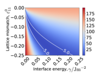
In our study, we demonstrated the performance of MF-LER using the Mg-based alloy data. On the basis of the analysis in our previous study [36], we set $h=5$ that was empirically inferred from the standard deviation of the aspect ratio in the experimental image. Figure 4 shows the heatmap of discrepancy and LER. We have three fidelity levels $M=3$, and the sampling costs of the low-, middle-, and highest-fidelity functions are $\lambda^{(1)}=5$, $\lambda^{(2)}=10$, and $\lambda^{(3)}=60$ minutes, respectively. For the candidate parameter $\boldsymbol{x}=(\gamma,\varepsilon_{11}^{0})^{\top}$, we used 250 equally spaced grids in $\varepsilon_{11}^{0}\in[-0.250,-0.001]$ and $\gamma\in[0.001,0.250]$ (J m^-2). Thus, we have a total of $N=62500$ candidates that require $3750000(=62500\times 60)$ minutes to compute all the points in the highest-fidelity function. To evaluate the usefulness of the low-fidelity observations, we compared MF-LER with two strategies that take samples only from the highest-fidelity function. The first approach is to use information gain (1) as the sampling criterion [36], called single-fidelity LER estimation (SF-LER), and the second approach is single-fidelity GP with random sampling, called SF-Random. For the initial points, SF-Random and SF-LER randomly selected five highest-fidelity points, and MF-LER randomly selected ten lowest fidelity points. For all approaches, a candidate $\boldsymbol{x}$ is classified as LER if $p(z_{\boldsymbol{x}}=1)\geq 0.5$. Detailed explanations of the GP are given in supplementary appendix B.

Figure 5 shows the sampling processes of MF-LER, SF-LER, and SF-Random. At “Cost 500,” MF-LER determines LER approximately, while SF-LER and SF-Random do not estimate LER accurately. At “Cost 1000,” MF-LER starts sampling from the highest-fidelity function and identifying LER in more detail. However, the predicted LER of SF-LER and SF-Random are still largely different from the truth. At “Cost 2000,” SF-LER starts identifying the rough shape of the LER, and the prediction of SF-Random is not still stable. At this cost, MF-LER provides almost precise LER estimation. The total cost 2000 is only approximately 0.05% ($\approx 2000/3750000\times 100$) of that used for exhaustive search on the highest-fidelity surface. This suggests that MF-LER is effective to accelerate the search process by reducing the sampling from expensive computations.

Figure 6 shows the quantitative performance evaluation. We evaluated the accuracy of LER estimation through the predicted binary label $z_{\boldsymbol{x}}$. Note that our objective was only to identify LER and not to approximate the entire discrepancy surface accurately that would require a higher number of samples. We used standard evaluation measures of the classification problem called recall, precision, and F-score. Because MF-LER sampled only from low-fidelity function values as initial points unlike the other two methods, the initial cost values of MF-LER in the plot are different from those of SF-LER and SF-Random. All the results are the averages of 10 runs with random initial points.

The left plot in Fig. 6 shows recall, defined by

This is the ratio of the number of LER points that are correctly identified over the number of points in the true LER. This evaluates how many LER points are correctly identified. At the beginning, recall was approximately $0.1$ for all sampling strategies owing to the absence of sampled points. However, MF-LER rapidly increased recall substantially faster than SF-LER and SF-Random. The middle plot in Fig. 6 shows precision, defined by

Precision has the same numerator as recall, but the denominator is the number of points predicted as the LER. This evaluates the specificity of prediction, which cannot be considered by recall. The precision values were higher than the recall values in the beginning, indicating that the large part of predicted LER was actually $y^{(M)}_{\boldsymbol{x}_{i}}\leq h$. Similar to recall, MF-LER was better than SF-LER and SF-Random at all the cost values. Because recall and precision have a tradeoff relationship, their harmonic mean, referred to as the F-score, is often used as a comprehensive evaluation criterion. The right plot of Fig. 6 shows the superior performance of MF-LER in terms of the F-score.

References

- [1] M. Kahlweit. Ostwald ripening of precipitates. Adv. Colloid Interface Sci., 5, 1975.
- [2] S. Ito, H. Nagao, A. Yamanaka, Y. Tsukada, T. Koyama, M. Kano, and J. Inoue. Data assimilation for massive autonomous systems based on a second-order adjoint method. Phys. Rev. E, 94, 2016.
- [3] S. Ito, H. Nagao, T. Kasuya, and J. Inoue. Grain growth prediction based on data assimilation by implementing 4DVar on multi-phase-field model. Sci. Technol. Adv. Mater., 18, 2017.
- [4] J. Zhang, S. O. Poulsen, J. W. Gibbs, P. W. Voorhees, and H. F. Poulsen. Determining material parameters using phase-field simulations and experiments. Acta Mater., 129, 2017.
- [5] K. Sasaki, A. Yamanaka, S. Ito, and H. Nagao. Data assimilation for phase-field models based on the ensemble Kalman filter. Comput. Mater. Sci., 141, 2018.
- [6] M. E. Thompson, C. S. Su, and P. W. Voorhees. Equilibrium shape of a misfitting precipitate. Acta Metall. Mater., 42, 1994.
- [7] I. Schmidt and D. Gross. The equilibrium shape of an elastically inhomogeneous inclusion. J. Mech. Phys. Solids, 45, 1997.
- [8] I. Schmidt, R. Mueller, and D. Gross. The effect of elastic inhomogeneity on equilibrium and stability of a two particle morphology. Mech. Mater., 30, 1998.
- [9] A. G. Khachaturyan. Theory of Structural Transformations in Solids. Dover, 2008.
- [10] D. A. Porter, K. E. Easterling, and M. Y. Sherif. Phase Transformations in Metals and Alloys 3rd edition. CRC Press, 2009.
- [11] J. B. Clark. Transmission electron microscopy study of age hardening in a Mg-5 wt.% Zn alloy. Acta Metall., 13, 1965.
- [12] J. S. Chun and J. G. Byrne. Precipitate strengthening mechanisms in magnesium zinc alloy single crystals. J. Mater. Sci., 4, 1969.
- [13] J. F. Nie and B. C. Muddle. Precipitation hardening of Mg-Ca(-Zn) alloys. Scr. Mater., 37, 1997.
- [14] S. Celotto. TEM study of continuous precipitation in Mg-9 wt.% Al-1 wt.% Zn alloy. Acta Mater., 48, 2000.
- [15] B. Smola, I. Stulíková, F. Buch, and B. L. Mordike. Structural aspects of high performance Mg alloys design. Mater. Sci. Eng. A, 324, 2002.
- [16] D. H. Ping, K. Hono, and J. F. Nie. Atom probe characterization of plate-like precipitates in a Mg-RE-Zn-Zr casting alloy. Scr. Mater., 48, 2003.
- [17] J. C. Oh, T. Ohkubo, T. Mukai, and K. Hono. TEM and 3DAP characterization of an age-hardened Mg-Ca-Zn alloy. Scr. Mater., 53, 2005.
- [18] J. F. Nie, X. Gao, and S. M. Zhu. Enhanced age hardening response and creep resistance of Mg-Gd alloys containing Zn. Scr. Mater., 53, 2005.
- [19] T. T. Sasaki, K. Oh-ishi, T. Ohkubo, and K. Hono. Enhanced age hardening response by the addition of Zn in Mg-Sn alloys. Scr. Mater., 55, 2006.
- [20] C. L. Mendis, C. J. Bettles, M. A. Gibson, and C. R. Hutchinson. An enhanced age hardening response in Mg-Sn based alloys containing Zn. Mater. Sci. Eng. A, 435-436, 2006.
- [21] C. L. Mendis, K. Oh-ishi, and K. Hono. Enhanced age hardening in a Mg-2.4 at.% Zn alloy by trace additions of Ag and Ca. Scr. Mater., 57, 2007.
- [22] T. T. Sasaki, T. Ohkubo, and K. Hono. Precipitation hardenable Mg-Bi-Zn alloys with prismatic plate precipitates. Scr. Mater., 61, 2009.
- [23] K. Oh-ishi, R. Watanabe, C. L. Mendis, and K. Hono. Age-hardening response of Mg-0.3 at.% Ca alloys with different Zn contents. Mater. Sci. Eng. A, 526, 2009.
- [24] T. T. Sasaki, K. Oh-ishi, T. Ohkubo, and K. Hono. Effect of double aging and microalloying on the age hardening behavior of a Mg-Sn-Zn alloy. Mater. Sci. Eng. A, 530, 2011.
- [25] C. L. Mendis, K. Oh-ishi, T. Ohkubo, and K. Hono. Precipitation of prismatic plates in Mg-0.3Ca alloys with In additions. Scr. Mater., 64, 2011.
- [26] C. L. Mendis, K. Oh-ishi, and K. Hono. Microalloying effect on the precipitation processes of Mg-Ca alloys. Metall. Mater. Trans. A, 43, 2012.
- [27] F. R. Elsayed, T. T. Sasaki, C. L. Mendis, T. Ohkubo, and K. Hono. Compositional optimization of Mg-Sn-Al alloys for higher age hardening response. Mater. Sci. Eng. A, 566, 2013.
- [28] T. Bhattacharjee, C. L. Mendis, K. Oh-ishi, T. Ohkubo, and K. Hono. The effect of Ag and Ca additions on the age hardening response of Mg-Zn alloys. Mater. Sci. Eng. A, 575, 2013.
- [29] T. Bhattacharjee, T. Nakata, T. T. Sasaki, S. Kamado, and K. Hono. Effect of microalloyed Zr on the extruded microstructure of Mg-6.2Zn-based alloys. Scr. Mater., 90-91, 2014.
- [30] T. T. Sasaki, F. Elsayed, T. Nakata, T. Ohkubo, S. Kamado, and K. Hono. Strong and ductile heat-treatable Mg-Sn-Zn-Al wrought alloys. Acta Mater., 99, 2015.
- [31] T. Nakata, C. Xu, R. Ajima, K. Shimizu, S. Hanaki, T. T. Sasaki, L. Ma, K. Hono, and S. Kamado. Strong and ductile age-hardening Mg-Al-Ca-Mn alloy that can be extruded as fast as aluminum alloys. Acta Mater., 130, 2017.
- [32] Y. Gao, H. Liu, R. Shi, N. Zhou, Z. Xu, Y.M. Zhu, J.F. Nie, and Y. Wang. Simulation study of precipitation in an Mg-Y-Nd alloy. Acta Mater., 60, 2012.
- [33] H. Liu, Y. Gao, J.Z. Liu, Y.M. Zhu, Y. Wang, and J.F. Nie. A simulation study of the shape of precipitates in Mg-Y and Mg-Gd alloys. Acta Mater., 61, 2013.
- [34] Y.Z. Ji, A. Issa, T.W. Heo, J.E. Saal, C. Wolverton, and L.-Q. Chen. Predicting precipitate morphology and evolution in Mg-RE alloys using a combination of first-principles calculations and phase-field modeling. Acta Mater., 76, 2014.
- [35] Y. Tsukada, Y. Beniya, and T. Koyama. Equilibrium shape of isolated precipitates in the -Mg phase. J. Alloy. Compd., 603, 2014.
- [36] Y. Tsukada, S. Takeno, M. Karasuyama, H. Fukuoka, M. Shiga, and T. Koyama. Estimation of material parameters based on precipitate shape: efficient identification of low-error region with gaussian process modeling. Sci. Rep., 9:15794, 2019.
- [37] G. Pilania, J.E. Gubernatis, and T. Lookman. Multi-fidelity machine learning models for accurate bandgap predictions of solids. Comput. Mater. Sci., 129:156 – 163, 2017.
- [38] M. C. Kennedy and A. O’Hagan. Predicting the output from a complex computer code when fast approximations are available. Biometrika, 87(1):1–13, 2000.
- [39] D. J. C. MacKay. Information Theory, Inference, and Learning Algorithms. Cambridge University Press, 2003.
- [40] T. Mura. Micromechanics of Defects in Solids 2nd rev. edition. Martinus Nijhoff, 1987.
- [41] The Japan Institute of Metals and Materials (ed.). Kinzoku Data Book 4th rev. edition. Maruzen, 2004.
- [42] C. E. Rasmussen and C. K. I. Williams. Gaussian Processes for Machine Learning (Adaptive Computation and Machine Learning). The MIT Press, 2005.
Appendix A Computational Details of Information Entropy
The first term of mutual information (1) is the entropy of the Bernoulli distribution. The probability mass function of this distribution is written as
where is the cumulative distribution function of the standard Gaussian distribution and is the threshold normalized by the predictive mean and variance of the highest-fidelity function at . Hence, the first term of (1) is calculated easily as
The second term of (1) is the expectation of the entropy of the Bernoulli distribution. We calculate this expectation using quadrature. First, we draw a sample from the current predictive distribution . To calculate the one-step-ahead predictive distribution of the highest-fidelity function , we consider the two-variable marginal distribution as follows:
where is the covariance between and . Through the conditional Gaussian distribution, we obtain
where,
Then, the entropy of is written as
where is the threshold normalized by the one-step-ahead predictive mean and variance of the highest-fidelity function at . Finally, we approximate the expectation using quadrature.
Appendix B Settings of Gaussian processes
We used the Gaussian kernel for both kernels and , which are defined as
where , and are hyperparameters. The variance of noise term is also a hyperparameter. We set . is optimized by marginal likelihood maximization [42] per iteration.