跳到论文正文
W Papers独立论文阅读器 arXiv:2003.13285 论文正文 计算阅读时间 · 0%
引用这篇论文根据当前论文元数据生成,正式投稿前建议核对。


License: arXiv.org perpetual non-exclusive license
arXiv:2003.13285v1 [math.CA] 30 Mar 2020

Fractional integrals, derivatives and integral equations with weighted Takagi–Landsberg functions

Vitalii Makogin    Yuliya Mishura
August 11, 2026
Abstract

In this paper we find fractional Riemann–Liouville derivatives for the Takagi-Landsberg functions. Moreover, we introduce their generalizations called weighted Takagi-Landsberg functions which have arbitrary bounded coefficients in the expansion under Schauder basis. The class of the weighted Takagi-Landsberg functions of order H>0H>0 on [0,1][0,1] coincides with the HH-Hölder continuous functions on [0,1][0,1]. Based on computed fractional integrals and derivatives of the Haar and Schauder functions, we get a new series representation of the fractional derivatives of a Hölder continuous function. This result allows to get the new formula of a Riemann-Stieltjes integral. The application of such series representation is the new method of numerical solution of the Volterra and linear integral equations driven by a Hölder continuous function.

1 Introduction

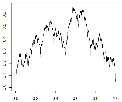
The aim of this paper is to get a broad class of continuous functions on [0,1], which are nowhere differentiable but have fractional derivatives. The prominent example is the Takagi–Landsberg function with Hurst parameter H>0H>0 introduced in [10], given by

xH​(t)=∑m=0∞2m⁡(12−H)​∑k=02m−1em,k​(t),t∈[0,1],x^{H}(t)=\sum_{m=0}^{\infty}2^{m\left(\frac{1}{2}-H\right)}\sum_{k=0}^{2^{m}-1}e_{m,k}(t),t\in[0,1], (1)

where {em,k,m∈ℕ0,k=0,…,2m−1}\{e_{m,k},m\in\mathbb{N}_{0},k=0,\ldots,2^{m}-1\} are the Faber-Schauder functions on [0,1]. In the present paper, we find the fractional derivatives of the Takagi-Landsberg functions, and for other properties we refer to the surveys [2] and [9]. In the case H=1/2,H=1/2, the function xHx^{H} is known as the Takagi function.

There are several generalizations of the function xH.x^{H}. In the paper of Mishura and Schied [13], the signed Takagi-Landsberg functions of the form

∑m=0∞2m⁡(12−H)​∑k=02m−1θm,k​em,k​(t),t∈[0,1]​ with ​θm,k∈{−1,+1}\sum_{m=0}^{\infty}2^{m\left(\frac{1}{2}-H\right)}\sum_{k=0}^{2^{m}-1}\theta_{m,k}e_{m,k}(t),t\in[0,1]\text{ with }\theta_{m,k}\in\{-1,+1\}

are considered. Their results concern the maximum, the maximizers, and the modulus of continuity. Particularly, it was shown that maxt∈[0,1]⁡xH​(t)=13​(1−2−H).\max_{t\in[0,1]}x^{H}(t)=\frac{1}{3(1-2^{-H})}. The case of H=1/2H=1/2 is considered in [16], where the connections to the Fölmer’s pathwise Itô calculus (e.g. [5]) is also described.

In the present paper we go further and introduce so-called weighted Takagi-Landsberg functions, for which we let θm,k\theta_{m,k} be arbitrary bounded coefficients. We show that such weighted Takagi-Landsberg functions coincides with the Hölder continuous functions which immediately gives the new series representation for them, which we call a Takagi-Landsberg representation. Then we compute the fractional Riemann–Liouville derivatives and integrals of the Faber-Schauder functions, and therefore we obtain the fractional derivatives of the (weighted) Takagi-Landsberg functions. Such a new series representation of the fractional derivative for Hölder continuous functions is very promising for further development of the continuous functions without derivatives. Particularly, the Takagi-Landsberg representation gives the new method for numerical solution of the integral equations involving Hölder continuous functions.

As an example, we consider the Volterra integral equation with fractional noise, called also fractional Langevin equation, e.g. [12, 4]. This equation is of interest for modeling of anomalous diffusion in physics (e.g. [11], [8]) and financial markets (e.g. [17]). Our method of its numerical solution allows to reduce it to the system of linear algebraic equations, which is computationally effective. We prove that the numerical solution of the fractional Langevin equation, due to our method, approaches the theoretical solution, which is illustrated by numerical examples.

We obtain also the series expansion of the Riemann-Stieltjes integral applying methodology based on fractional Rieman-Liuville integrals introduced in [18] and developed in [14]. As an illustration we consider the linear differential equation driven by Hölder continuous function and prove that its numerical solution due to our method tends to the exact solution in the specific norm. This result are supported also by numerical examples.

The paper is organized as follows. In Section 2, we recal some basic definitions from fractional calculus and Schauder basis. In Section 3, we compute fractional Riemann–Liouville integrals and derivatives of the Haar (Section 3.1) and the Faber-Schauder (Section 3.2) functions. In Section 4, we introduce the weighted Takagi-Landsberg functions and obtain the series representations of their Riemann–Liouville derivatives. The series expansion of the Riemann-Stieltjes integral is given in Section 5. In Section 6, we consider the application of the Takagi-Landsberg representation for the solution of the Volterra integral (Section 6.1) and linear differential (Section 6.2) equations. The numerical results are presented in Sections 6.3 and 6.4.

2 Preliminaries

First we recall the definitions of fractional Riemann-Liouville integrals and derivatives and their basic properties. Let f∈L1​([0,T]).f\in L_{1}([0,T]). We define left- and right-sided fractional integrals of order α>0\alpha>0 on (0,T)(0,T) by

[I0+α​f]​(t)\displaystyle[I_{0+}^{\alpha}f](t) :=1Γ⁡(α)​∫0t(t−u)α−1​f​(u)​𝑑u,\displaystyle:=\frac{1}{\Gamma(\alpha)}\int_{0}^{t}(t-u)^{\alpha-1}f(u)du, (2)
[IT−α​f]​(t)\displaystyle[I_{T-}^{\alpha}f](t) :=1Γ⁡(α)​∫tT(u−t)α−1​f​(u)​𝑑u,\displaystyle:=\frac{1}{\Gamma(\alpha)}\int_{t}^{T}(u-t)^{\alpha-1}f(u)du, (3)

respectively (cf. [15, Definition 2.1]).

Define the spaces of functions that can be represented as fractional integrals:

I+α​(Lp​([0,T])):={f∈L1​([0,T]):∃φ∈Lp​([0,T])​ such that ​f=I0+α​φ},I_{+}^{\alpha}(L_{p}([0,T])):=\{f\in L_{1}([0,T]):\exists\varphi\in L_{p}([0,T])\text{ such that }f=I_{0+}^{\alpha}\varphi\},
I−α​(Lp​([0,T])):={f∈L1​([0,T]):∃φ∈Lp​([0,T])​ such that ​f=IT−α​φ}.I_{-}^{\alpha}(L_{p}([0,T])):=\{f\in L_{1}([0,T]):\exists\varphi\in L_{p}([0,T])\text{ such that }f=I_{T-}^{\alpha}\varphi\}.

From [15, formula (2.19)] it follows that I+α​(Lp​([0,T]))=I−α​(Lp​([0,T]))I_{+}^{\alpha}(L_{p}([0,T]))=I_{-}^{\alpha}(L_{p}([0,T])) for 1<p<1α.1<p<\frac{1}{\alpha}.

For the functions from I+α​(L1​([0,T]))=I−α​(L1​([0,T]))I_{+}^{\alpha}(L_{1}([0,T]))=I_{-}^{\alpha}(L_{1}([0,T])) we define the left- and right-sided fractional Riemann-Liouville derivatives on (0,T)(0,T) of order α\alpha by

[D0+α​f]​(t)\displaystyle[D_{0+}^{\alpha}f](t) =1Γ⁡(1−α)​dd​t​∫0t(t−u)−α​f​(u)​𝑑u\displaystyle=\frac{1}{\Gamma(1-\alpha)}\frac{d}{dt}\int_{0}^{t}(t-u)^{-\alpha}f(u)du (4)
[DT−α​f]​(t)\displaystyle[D_{T-}^{\alpha}f](t) =−1Γ⁡(1−α)dd​t∫tT(u−t)−αf(u)du.\displaystyle=-\frac{1}{\Gamma(1-\alpha)}\frac{d}{dt}\int_{t}^{T}(u-t)^{-\alpha}f(u)du. (5)

Recall that the Faber–Schauder functions are defined as

e∅(t):=t,e0,0(t):=(min{t,1−t})+,em,k(t):=2−m/2e0,0(2mt−k)e_{\emptyset}(t):=t,\quad e_{0,0}(t):=(\min\{t,1-t\})^{+},\quad e_{m,k}(t):=2^{-m/2}e_{0,0}(2^{m}t-k)

for t∈ℝ,m∈ℕ,k∈ℕ0.t\in\mathbb{R},m\in\mathbb{N},k\in\mathbb{N}_{0}. They can be expressed in terms of Haar functions Hm,kH_{m,k} as

em,k​(t)=∫0tHm,k​(s)​𝑑s=[I0+1​Hm,k]​(t), where ​Hm,k​(s)=2m2​𝟙Jm,k​(s)−2m2​𝟙Jm,k+0.5​(s),e_{m,k}(t)=\int_{0}^{t}H_{m,k}(s)ds=[I_{0+}^{1}H_{m,k}](t),\text{ where }H_{m,k}(s)=2^{\frac{m}{2}}\mathbbm{1}_{J_{m,k}}(s)-2^{\frac{m}{2}}\mathbbm{1}_{J_{m,k+0.5}}(s), (6)

and Jm,t:=(t2m,t+0.52m],J_{m,t}:=\left(\frac{t}{2^{m}},\frac{t+0.5}{2^{m}}\right], m∈ℕ0,k=0,…,2m−1,t∈[0,1].m\in\mathbb{N}_{0},k=0,\ldots,2^{m}-1,t\in[0,1].

The Faber-Schauder functions form a Schauder basis in C⁡([0,1])C([0,1]) and produce the following expansion of a function f∈C⁡([0,1])f\in C([0,1]) (e.g. [7])

f⁡(t)\displaystyle f(t) =f⁡(0)+(f⁡(1)−f⁡(0))​t+∑m=0∞∑k=02m−12m2​am,k​em,k​(t),t∈[0,1],\displaystyle=f(0)+(f(1)-f(0))t+\sum_{m=0}^{\infty}\sum_{k=0}^{2^{m}-1}2^{\frac{m}{2}}a_{m,k}e_{m,k}(t),t\in[0,1], (7)

with coefficients

am,k=2​f​(k+0.52m)−f⁡(k+12m)−f⁡(k2m).a_{m,k}=2f\left(\frac{k+0.5}{2^{m}}\right)-f\left(\frac{k+1}{2^{m}}\right)-f\left(\frac{k}{2^{m}}\right).

3 Fractional derivatives of the Takagi–Landsberg function

3.1 Haar functions

In this section, we calculate the fractional integrals and derivatives of the Haar functions.

Lemma 3.1.

Let α>0,\alpha>0, T>0,T>0, k,m∈ℕ0k,m\in\mathbb{N}_{0} and 0≤k<2m.0\leq k<2^{m}. Then for t∈(0,1)t\in(0,1) we have

I0+α​Hm,k​(t)=2m2Γ⁡(1+α)​((t−k2m)+α−2​(t−k+0.52m)+α+(t−k+12m)+α),I_{0+}^{\alpha}H_{m,k}(t)=\frac{2^{\frac{m}{2}}}{\Gamma(1+\alpha)}\left(\left(t-\frac{k}{2^{m}}\right)^{\alpha}_{+}-2\left(t-\frac{k+0.5}{2^{m}}\right)^{\alpha}_{+}+\left(t-\frac{k+1}{2^{m}}\right)^{\alpha}_{+}\right), (8)

and

IT−α​Hm,k​(t)=2m2Γ⁡(1+α)​(2​(T∧k+0.52m−t)+α−(T∧k2m−t)+α−(T∧k+12m−t)+α),I_{T-}^{\alpha}H_{m,k}(t)=\frac{2^{\frac{m}{2}}}{\Gamma(1+\alpha)}\left(2\left(T\wedge\frac{k+0.5}{2^{m}}-t\right)_{+}^{\alpha}-\left(T\wedge\frac{k}{2^{m}}-t\right)_{+}^{\alpha}-\left(T\wedge\frac{k+1}{2^{m}}-t\right)_{+}^{\alpha}\right), (9)

for t∈(0,T).t\in(0,T).

Proof.

If t<k2m,t<\frac{k}{2^{m}}, then I0+α​Hm,k​(t)=0.I_{0+}^{\alpha}H_{m,k}(t)=0. Let t∈Jm,k,t\in J_{m,k}, then

I0+α​Hm,k​(t)=2m2Γ⁡(α)​∫k/2mt(t−u)α−1​𝑑u=2m2Γ⁡(1+α)​(t−k2m)α.\displaystyle I_{0+}^{\alpha}H_{m,k}(t)=\frac{2^{\frac{m}{2}}}{\Gamma(\alpha)}\int_{k/2^{m}}^{t}(t-u)^{\alpha-1}du=\frac{2^{\frac{m}{2}}}{\Gamma(1+\alpha)}\left(t-\frac{k}{2^{m}}\right)^{\alpha}. (10)

Let t∈Jm,k+0.5,t\in J_{m,k+0.5}, then

I0+α​Hm,k​(t)\displaystyle I_{0+}^{\alpha}H_{m,k}(t) =2m2Γ⁡(α)​(∫k/2m(k+0.5)/2m(t−u)α−1​𝑑u−∫(k+0.5)/2mt(t−u)α−1​𝑑u)\displaystyle=\frac{2^{\frac{m}{2}}}{\Gamma(\alpha)}\left(\int_{k/2^{m}}^{(k+0.5)/2^{m}}(t-u)^{\alpha-1}du-\int_{(k+0.5)/2^{m}}^{t}(t-u)^{\alpha-1}du\right)
=2m2Γ⁡(1+α)​((t−k2m)α−2​(t−k+0.52m)α).\displaystyle=\frac{2^{\frac{m}{2}}}{\Gamma(1+\alpha)}\left(\left(t-\frac{k}{2^{m}}\right)^{\alpha}-2\left(t-\frac{k+0.5}{2^{m}}\right)^{\alpha}\right). (11)

If t>k+12m,t>\frac{k+1}{2^{m}}, then

I0+α​Hm,k​(t)\displaystyle I_{0+}^{\alpha}H_{m,k}(t) =2m2Γ⁡(α)​(∫k/2m(k+0.5)/2m(t−u)α−1​𝑑u−∫(k+0.5)/2m(k+1)/2m(t−u)α−1​𝑑u)\displaystyle=\frac{2^{\frac{m}{2}}}{\Gamma(\alpha)}\left(\int_{k/2^{m}}^{(k+0.5)/2^{m}}(t-u)^{\alpha-1}du-\int_{(k+0.5)/2^{m}}^{(k+1)/2^{m}}(t-u)^{\alpha-1}du\right)
=2m2Γ⁡(1+α)​((t−k2m)α−2​(t−k+0.52m)α+(t−k+12m)α).\displaystyle=\frac{2^{\frac{m}{2}}}{\Gamma(1+\alpha)}\left(\left(t-\frac{k}{2^{m}}\right)^{\alpha}-2\left(t-\frac{k+0.5}{2^{m}}\right)^{\alpha}+\left(t-\frac{k+1}{2^{m}}\right)^{\alpha}\right). (12)

Summarizing (10)–(12), we get the statement (8).

Now prove relation (9). Obviously, if T<k2mT<\frac{k}{2^{m}} or t>k+12m,t>\frac{k+1}{2^{m}}, then IT−α​Hm,k​(t)=0.I_{T-}^{\alpha}H_{m,k}(t)=0. Let t∈Jm,k+0.5,t\in J_{m,k+0.5}, then

IT−αHm,k(t)=−2m2Γ⁡(α)∫tT∧k+12m(u−t)α−1du=−2m2Γ⁡(1+α)(T∧k+12m−t)α.\displaystyle I_{T-}^{\alpha}H_{m,k}(t)=-\frac{2^{\frac{m}{2}}}{\Gamma(\alpha)}\int_{t}^{T\wedge\frac{k+1}{2^{m}}}(u-t)^{\alpha-1}du=-\frac{2^{\frac{m}{2}}}{\Gamma(1+\alpha)}\left(T\wedge\frac{k+1}{2^{m}}-t\right)^{\alpha}. (13)

Let t∈Jm,k,t\in J_{m,k}, then

IT−α​Hm,k​(t)\displaystyle I_{T-}^{\alpha}H_{m,k}(t) =2m2Γ⁡(α)​(∫tT∧k+0.52m(u−t)α−1​𝑑u−∫T∧k+0.52mT∧k+12m(u−t)α−1​𝑑u)\displaystyle=\frac{2^{\frac{m}{2}}}{\Gamma(\alpha)}\left(\int_{t}^{T\wedge\frac{k+0.5}{2^{m}}}(u-t)^{\alpha-1}du-\int_{T\wedge\frac{k+0.5}{2^{m}}}^{T\wedge\frac{k+1}{2^{m}}}(u-t)^{\alpha-1}du\right)
=2m2Γ⁡(1+α)​(2​(T∧k+0.52m−t)α−(T∧k+12m−t)α).\displaystyle=\frac{2^{\frac{m}{2}}}{\Gamma(1+\alpha)}\left(2\left(T\wedge\frac{k+0.5}{2^{m}}-t\right)^{\alpha}-\left(T\wedge\frac{k+1}{2^{m}}-t\right)^{\alpha}\right). (14)

If t<k2m,t<\frac{k}{2^{m}}, then

IT−α​Hm,k​(t)=2m2Γ⁡(α)​(∫T∧k2mT∧k+0.52m(u−t)α−1​𝑑u−∫T∧k+0.52mT∧k+12m(u−t)α−1​𝑑u)\displaystyle I_{T-}^{\alpha}H_{m,k}(t)=\frac{2^{\frac{m}{2}}}{\Gamma(\alpha)}\left(\int_{T\wedge\frac{k}{2^{m}}}^{T\wedge\frac{k+0.5}{2^{m}}}(u-t)^{\alpha-1}du-\int_{T\wedge\frac{k+0.5}{2^{m}}}^{T\wedge\frac{k+1}{2^{m}}}(u-t)^{\alpha-1}du\right)
=2m2Γ⁡(1+α)​(−(T∧k2m−t)α+2​(T∧k+0.52m−t)α−(T∧k+12m−t)α).\displaystyle=\frac{2^{\frac{m}{2}}}{\Gamma(1+\alpha)}\left(-\left(T\wedge\frac{k}{2^{m}}-t\right)^{\alpha}+2\left(T\wedge\frac{k+0.5}{2^{m}}-t\right)^{\alpha}-\left(T\wedge\frac{k+1}{2^{m}}-t\right)^{\alpha}\right). (15)

Summarizing (13)–(15), we get the statement (9). ∎

For m∈ℕ0,k=0,…,2m−1,H>0m\in\mathbb{N}_{0},k=0,\ldots,2^{m}-1,H>0 denote by

τ1,2m+kα​(t)=(t−k2m)+α−2​(t−k+0.52m)+α+(t−k+12m)+αΓ⁡(1+α),t∈[0,1],α≥0,\tau^{\alpha}_{1,2^{m}+k}(t)=\frac{\left(t-\frac{k}{2^{m}}\right)_{+}^{\alpha}-2\left(t-\frac{k+0.5}{2^{m}}\right)_{+}^{\alpha}+\left(t-\frac{k+1}{2^{m}}\right)_{+}^{\alpha}}{\Gamma(1+\alpha)},t\in[0,1],\alpha\geq 0, (16)

and

τ2,2m+kα​(t,T)=2​(T∧k+0.52m−t)+α−(T∧k2m−t)+α−(T∧k+12m−t)+αΓ⁡(1+α),[0,T],α≥0.\tau^{\alpha}_{2,2^{m}+k}(t,T)=\frac{2\left(T\wedge\frac{k+0.5}{2^{m}}-t\right)_{+}^{\alpha}-\left(T\wedge\frac{k}{2^{m}}-t\right)_{+}^{\alpha}-\left(T\wedge\frac{k+1}{2^{m}}-t\right)_{+}^{\alpha}}{\Gamma(1+\alpha)},[0,T],\alpha\geq 0.

Then I0+α​Hm,k​(t)=2m2​τ1,2m+kα​(t)I_{0+}^{\alpha}H_{m,k}(t)=2^{\frac{m}{2}}\tau^{\alpha}_{1,2^{m}+k}(t) and IT−α​Hm,k​(t)=2m2​τ2,2m+kα​(t,T).I_{T-}^{\alpha}H_{m,k}(t)=2^{\frac{m}{2}}\tau^{\alpha}_{2,2^{m}+k}(t,T).

Remark 3.1.

We give immediate bounds for τ1,2m+kα\tau^{\alpha}_{1,2^{m}+k} and τ2,2m+kα.\tau^{\alpha}_{2,2^{m}+k}. For instance, for any m∈ℕ0m\in\mathbb{N}_{0} and k=0,…,2m−1k=0,\ldots,2^{m-1} we have

|τ1,2m+kα​(t)|=|I0+α​2−m2​Hm,k​(t)|≤I0+α​[𝟙Jm,k+𝟙Jm,k+0.5]​(t)≤I0+α​[𝟙Jm,k+𝟙Jm,k+0.5]​(1)\displaystyle|\tau^{\alpha}_{1,2^{m}+k}(t)|=|I_{0+}^{\alpha}2^{-\frac{m}{2}}H_{m,k}(t)|\leq I_{0+}^{\alpha}[\mathbbm{1}_{J_{m,k}}+\mathbbm{1}_{J_{m,k+0.5}}](t)\leq I_{0+}^{\alpha}[\mathbbm{1}_{J_{m,k}}+\mathbbm{1}_{J_{m,k+0.5}}](1)
=1Γ⁡(α)​∫k2mk+12m(1−u)α−1​𝑑u=1Γ⁡(1+α)​((1−k+12m)α−(1−k2m)α)≤2−m​αΓ⁡(1+α).\displaystyle=\frac{1}{\Gamma(\alpha)}\int_{\frac{k}{2^{m}}}^{\frac{k+1}{2^{m}}}(1-u)^{\alpha-1}du=\frac{1}{\Gamma(1+\alpha)}\left(\left(1-\frac{k+1}{2^{m}}\right)^{\alpha}-\left(1-\frac{k}{2^{m}}\right)^{\alpha}\right)\leq\frac{2^{-m\alpha}}{\Gamma(1+\alpha)}.

Similarly, we get that |τ1,2m+kα​(t)|≤IT−α​𝟙Jm,k∪Jm,k+0.5​(t)≤I1−α​𝟙Jm,k∪Jm,k+0.5​(0)≤2−m​αΓ⁡(1+α).|\tau^{\alpha}_{1,2^{m}+k}(t)|\leq I_{T-}^{\alpha}\mathbbm{1}_{J_{m,k}\cup J_{m,k+0.5}}(t)\leq I_{1-}^{\alpha}\mathbbm{1}_{J_{m,k}\cup J_{m,k+0.5}}(0)\leq\frac{2^{-m\alpha}}{\Gamma(1+\alpha)}.

Remark 3.2.

One can observe that functions τ1,2m+kα\tau^{\alpha}_{1,2^{m}+k} and τ2,2m+kα\tau^{\alpha}_{2,2^{m}+k} can be written in terms of a fractional Gaussian noise with Hurst index H∈(0,1),H\in(0,1), that is a centered Gaussian process with the covariance function

𝐄⁡[YH​(t)​YH​(0)]=CH​(t)=12​(|t+1|2​H−2​|t|2​H+|t−1|2​H),t∈ℝ.\mathbf{E}[Y^{H}(t)Y^{H}(0)]=C_{H}(t)=\frac{1}{2}\left(|t+1|^{2H}-2|t|^{2H}+|t-1|^{2H}\right),t\in\mathbb{R}.

Indeed,

τ1,2m+kα​(t)=21−α2m​α​Γ​(1+α)​Cα/2​(2m+1​t−2​k−1), if ​t≥k+12m,\tau^{\alpha}_{1,2^{m}+k}(t)=\frac{2^{1-\alpha}}{2^{m\alpha}\Gamma(1+\alpha)}C_{\alpha/2}\left(2^{m+1}t-2k-1\right),\text{ if }t\geq\frac{k+1}{2^{m}},

and

τ2,2m+kα​(t,T)=−21−α2m​α​Γ​(1+α)​Cα/2​(2​k+1−2m+1​t), if ​t≤k2m​ and ​T≥k+12m.\tau^{\alpha}_{2,2^{m}+k}(t,T)=-\frac{2^{1-\alpha}}{2^{m\alpha}\Gamma(1+\alpha)}C_{\alpha/2}\left(2k+1-2^{m+1}t\right),\text{ if }t\leq\frac{k}{2^{m}}\text{ and }T\geq\frac{k+1}{2^{m}}.

Since α2∈(0,12)\frac{\alpha}{2}\in\left(0,\frac{1}{2}\right) if α∈(0,1),\alpha\in(0,1), we can study properties of the integrals I0+α​Hm,kI_{0+}^{\alpha}H_{m,k} and IT−α​Hm,kI_{T-}^{\alpha}H_{m,k} using the known results about CHC_{H} with H<1/2.H<1/2. For instance, it is known that CH​(t)<0C_{H}(t)<0 if t≥1t\geq 1 and H∈(0,1/2).H\in(0,1/2).

Further, we use the fact that function CHC_{H} in the case H<1/2H<1/2 is absolutely integrable and monotonically increasing on [1,+∞),[1,+\infty), e.g. [3, Section 3.2]

Remark 3.3.

We provide some auxiliary bounds for functions τ1,2m+kα\tau^{\alpha}_{1,2^{m}+k} and τ2,2m+kα.\tau^{\alpha}_{2,2^{m}+k}. Let α∈(0,1),\alpha\in(0,1), then Cα2​(x)C_{\frac{\alpha}{2}}(x) is negative and monotonically increasing for x≥1,x\geq 1, which gives that |Cα2​(x)|≤|Cα2​(⌊x⌋)|,x≥1.|C_{\frac{\alpha}{2}}(x)|\leq|C_{\frac{\alpha}{2}}(\left\lfloor x\right\rfloor)|,x\geq 1. Therefore, τ1,2m+kα​(t)\tau^{\alpha}_{1,2^{m}+k}(t) is negative for k≤⌊2m​t⌋−1k\leq\left\lfloor 2^{m}t\right\rfloor-1 and

2m​α​Γ​(1+α)21−α​|τ1,2m+kα​(t)|=|Cα/2​(2m+1​t−2​k−1)|≤|Cα/2​(2​⌊2m​t⌋−2​k−1)|.\displaystyle\frac{2^{m\alpha}\Gamma(1+\alpha)}{2^{1-\alpha}}|\tau^{\alpha}_{1,2^{m}+k}(t)|=\left|C_{\alpha/2}\left(2^{m+1}t-2k-1\right)\right|\leq\left|C_{\alpha/2}\left(2\left\lfloor 2^{m}t\right\rfloor-2k-1\right)\right|.

Similarly, if ⌊2m​t⌋+1≤k≤⌊2m​T⌋−1,\left\lfloor{2^{m}t}\right\rfloor+1\leq k\leq\left\lfloor{2^{m}T}\right\rfloor-1, then

2m​α​Γ​(1+α)21−α​|τ2,2m+kα​(t,T)|=|Cα/2​(1+2​k−2m+1​t)|≤|Cα/2​(2​k−⌊2m​t⌋−1)|.\displaystyle\frac{2^{m\alpha}\Gamma(1+\alpha)}{2^{1-\alpha}}|\tau^{\alpha}_{2,2^{m}+k}(t,T)|=\left|C_{\alpha/2}\left(1+2k-2^{m+1}t\right)\right|\leq\left|C_{\alpha/2}\left(2k-\left\lfloor 2^{m}t\right\rfloor-1\right)\right|.

3.2 The Faber-Schauder functions

Here, we find the fractional integrals and derivatives of the Faber-Schauder functions.

Lemma 3.2.

Let α∈(0,1),\alpha\in(0,1), T>0,T>0, k,m∈ℕ0k,m\in\mathbb{N}_{0} and 0≤k<2m.0\leq k<2^{m}. Then for t∈(0,1)t\in(0,1) we have I0+α​em,k​(t)=I0+1+α​Hm,k​(t)I_{0+}^{\alpha}e_{m,k}(t)=I_{0+}^{1+\alpha}H_{m,k}(t) and IT−α​em,k​(t)=em,k​(T)​IT−α​𝟙[0,1]​(t)−IT−1+α​Hm,k​(t)I_{T-}^{\alpha}e_{m,k}(t)=e_{m,k}(T)I_{T-}^{\alpha}\mathbbm{1}_{[0,1]}(t)-I_{T-}^{1+\alpha}H_{m,k}(t), t∈(0,T).t\in(0,T).

Proof.

It follows from [15, formula (2.65)] that I0+α​em,k=I0+α​I0+1​em,k=I0+1+α​Hm,k.I_{0+}^{\alpha}e_{m,k}=I_{0+}^{\alpha}I_{0+}^{1}e_{m,k}=I_{0+}^{1+\alpha}H_{m,k}. Consider IT−α​em,k=IT−α​I0+1​Hm,k.I_{T-}^{\alpha}e_{m,k}=I_{T-}^{\alpha}I_{0+}^{1}H_{m,k}. It equals

1Γ⁡(α)​∫tT(∫0sHm,k​(z)​𝑑z)​(s−t)α−1​𝑑s=1Γ⁡(α)​∫0THm,k​(z)​(∫z∨tT(s−t)α−1​𝑑s)​𝑑z\displaystyle\frac{1}{\Gamma(\alpha)}\int_{t}^{T}\left(\int_{0}^{s}H_{m,k}(z)dz\right)(s-t)^{\alpha-1}ds=\frac{1}{\Gamma(\alpha)}\int_{0}^{T}H_{m,k}(z)\left(\int_{z\vee t}^{T}(s-t)^{\alpha-1}ds\right)dz
=1Γ⁡(1+α)​∫0THm,k​(z)​((T−t)α−(z−t)+α​𝑑s)​𝑑z=em,k​(T)Γ⁡(1+α)​(T−t)α−IT−1+α​Hm,k​(t).\displaystyle=\frac{1}{\Gamma(1+\alpha)}\int_{0}^{T}H_{m,k}(z)\left((T-t)^{\alpha}-(z-t)_{+}^{\alpha}ds\right)dz=\frac{e_{m,k}(T)}{\Gamma(1+\alpha)}(T-t)^{\alpha}-I_{T-}^{1+\alpha}H_{m,k}(t).

Finally, we note that 1Γ⁡(1+α)​(T−t)α=IT−α​𝟙[0,1]​(t)\frac{1}{\Gamma(1+\alpha)}(T-t)^{\alpha}=I_{T-}^{\alpha}\mathbbm{1}_{[0,1]}(t) ∎

Proposition 3.1.

Let α∈(0,1),\alpha\in(0,1), T>0,T>0, k,m∈ℕ0k,m\in\mathbb{N}_{0} and 0≤k<2m.0\leq k<2^{m}. Then for t∈(0,1)t\in(0,1) we have

D0+α​em,k​(t)=2m⁡(α−12)Γ⁡(2−α)​((2m​t−k)+1−α−2​(2m​t−k−0.5)+1−α+(2m​t−k−1)+1−α),D_{0+}^{\alpha}e_{m,k}(t)=\frac{2^{m(\alpha-\frac{1}{2})}}{\Gamma(2-\alpha)}\left((2^{m}t-k)^{1-\alpha}_{+}-2(2^{m}t-k-0.5)^{1-\alpha}_{+}+(2^{m}t-k-1)^{1-\alpha}_{+}\right), (17)

and

DT−α​em,k​(t)=em,k​(T)​DT−α​𝟙[0,1]​(t)−IT−1−α​Hm,k​(t),t∈(0,T).\displaystyle D_{T-}^{\alpha}e_{m,k}(t)={e_{m,k}(T)}D_{T-}^{\alpha}\mathbbm{1}_{[0,1]}(t)-I_{T-}^{1-\alpha}H_{m,k}(t),t\in(0,T). (18)
Proof.

Formula (17) follows directly from Lemma 3.2 and formula (8), since D0+α​em,k=D0+α​I0+1​Hm,k=I0+1−α​Hm,k,D_{0+}^{\alpha}e_{m,k}=D_{0+}^{\alpha}I_{0+}^{1}H_{m,k}=I_{0+}^{1-\alpha}H_{m,k}, e.g. [15, formula 2.65].

We obtain the derivative DT−αD_{T-}^{\alpha} from the relation DT−α​em,k​(t)=−dd​t​[IT−1−α​em,k]​(t).D_{T-}^{\alpha}e_{m,k}(t)=-\frac{d}{dt}[I_{T-}^{1-\alpha}e_{m,k}](t). Thus, we have from Lemma 3.2 and formula (9) that

DT−α​em,k​(t)=−dd​t​(em,k​(T)​IT−1−α​𝟙[0,1]​(t)−IT−2−α​Hm,k​(t))=em,k​(T)Γ⁡(1−α)​(T−t)−α\displaystyle D_{T-}^{\alpha}e_{m,k}(t)=-\frac{d}{dt}\left(e_{m,k}(T)I_{T-}^{1-\alpha}\mathbbm{1}_{[0,1]}(t)-I_{T-}^{2-\alpha}H_{m,k}(t)\right)=\frac{e_{m,k}(T)}{\Gamma(1-\alpha)}(T-t)^{-\alpha}
+dd​t​IT−1−α​IT−1​Hm,k​(t)=em,k​(T)Γ⁡(1−α)​(T−t)−α−DT−α​IT−1​Hm,k​(t)\displaystyle+\frac{d}{dt}I_{T-}^{1-\alpha}I_{T-}^{1}H_{m,k}(t)=\frac{e_{m,k}(T)}{\Gamma(1-\alpha)}(T-t)^{-\alpha}-D_{T-}^{\alpha}I_{T-}^{1}H_{m,k}(t)
=em,k​(T)​DT−α​𝟙[0,1]​(t)−IT−1−α​Hm,k​(t).\displaystyle=e_{m,k}(T)D_{T-}^{\alpha}\mathbbm{1}_{[0,1]}(t)-I_{T-}^{1-\alpha}H_{m,k}(t).

∎

Remark 3.4.

We can write the fractional derivatives D0+α​em,kD_{0+}^{\alpha}e_{m,k} and DT−α​em,kD_{T-}^{\alpha}e_{m,k} as

D0+α​em,k​(t)=2m2​τ1,2m+k1−α​(t),DT−α​em,k​(t)=em,k​(T)Γ⁡(1−α)​(T−t)−α−2m2​τ2,2m+k1−α​(t,T).D_{0+}^{\alpha}e_{m,k}(t)=2^{\frac{m}{2}}\tau^{1-\alpha}_{1,2^{m}+k}(t),\quad D_{T-}^{\alpha}e_{m,k}(t)=\frac{e_{m,k}(T)}{\Gamma(1-\alpha)}(T-t)^{-\alpha}-2^{\frac{m}{2}}\tau^{1-\alpha}_{2,2^{m}+k}(t,T). (19)
Lemma 3.3.

1) Let a series ∑n=0∞an​(t),t∈[0,T]\sum_{n=0}^{\infty}a_{n}(t),t\in[0,T] be uniformly bounded by a non-negative function A∈L1​[0,T],A\in L_{1}[0,T], then

I0+α​(∑n=0∞an)​(t)=∑n=0∞(I0+α​an)​(t),t∈[0,T].I^{\alpha}_{0+}\left(\sum_{n=0}^{\infty}a_{n}\right)(t)=\sum_{n=0}^{\infty}\left(I^{\alpha}_{0+}a_{n}\right)(t),t\in[0,T]. (20)

2) Let ∑n=0∞an​(t),t∈[0,T]\sum_{n=0}^{\infty}a_{n}(t),t\in[0,T] be a convergent in L1​[0,T]L_{1}[0,T] series with an∈I+α​(L1​[0,T]),n≥0.a_{n}\in I_{+}^{\alpha}(L_{1}[0,T]),n\geq 0. If the exists a summable sequence bn≥0,n≥0b_{n}\geq 0,n\geq 0 such that |(D0+α​an)​(t)|≤bn|\left(D^{\alpha}_{0+}a_{n}\right)(t)|\leq b_{n} for all t∈[0,T]t\in[0,T], then

D0+α​(∑n=0∞an)​(t)=∑n=0∞(D0+α​an)​(t),t∈[0,T].D^{\alpha}_{0+}\left(\sum_{n=0}^{\infty}a_{n}\right)(t)=\sum_{n=0}^{\infty}\left(D^{\alpha}_{0+}a_{n}\right)(t),t\in[0,T]. (21)
Proof.

1) The first statement follows from the Lebesgue dominated convergence theorem, that is

∫0t(t−z)α−1​(∑n=0∞|an​(z)|)​𝑑z≤∫0t(t−z)α−1​A​(z)​𝑑z=Γ⁡(α)​(I0+α​A)​(t),\int_{0}^{t}(t-z)^{\alpha-1}\left(\sum_{n=0}^{\infty}|a_{n}(z)|\right)dz\leq\int_{0}^{t}(t-z)^{\alpha-1}A(z)dz=\Gamma(\alpha)\left(I_{0+}^{\alpha}A\right)(t),

where I0+α​A​(t)I_{0+}^{\alpha}A(t) is finite for almost all t∈(0,T)t\in(0,T) due to ‖I0+α​A‖L1​[0,T]<∞,\|I^{\alpha}_{0+}A\|_{L_{1}[0,T]}<\infty, e.g [15, Theorem 2.6].

2) Note that (D0+α​an)​(t)=dd​t​(I0+1−α​an)​(t)\left(D_{0+}^{\alpha}a_{n}\right)(t)=\frac{d}{dt}\left(I^{1-\alpha}_{0+}a_{n}\right)(t). Since ∑n=0∞an∈L1​[0,T],\sum_{n=0}^{\infty}a_{n}\in L_{1}[0,T], we have from the first part that I0+1−α​(∑n=0∞an)​(t)=∑n=0∞(I0+1−α​an)​(t).I^{1-\alpha}_{0+}\left(\sum_{n=0}^{\infty}a_{n}\right)(t)=\sum_{n=0}^{\infty}\left(I^{1-\alpha}_{0+}a_{n}\right)(t). Then

D0+α​(∑n=0∞an)​(t)=dd​t​(I0+1−α​(∑n=0∞an))​(t)=dd​t​(∑n=0∞(I0+1−α​an))​(t).\displaystyle D^{\alpha}_{0+}\left(\sum_{n=0}^{\infty}a_{n}\right)(t)=\frac{d}{dt}\left(I^{1-\alpha}_{0+}\left(\sum_{n=0}^{\infty}a_{n}\right)\right)(t)=\frac{d}{dt}\left(\sum_{n=0}^{\infty}\left(I^{1-\alpha}_{0+}a_{n}\right)\right)(t).

Since ∑n=0∞|dd​t​(I0+1−α​an)​(t)|≤∑n=0∞bn<∞,\sum_{n=0}^{\infty}\left|\frac{d}{dt}\left(I^{1-\alpha}_{0+}a_{n}\right)(t)\right|\leq\sum_{n=0}^{\infty}b_{n}<\infty, we have

dd​t​(∑n=0∞(I0+1−α​an))​(t)=∑n=0∞dd​t​(I0+1−α​an)​(t)=∑n=0∞(D0+α​an)​(t),t∈[0,T].\displaystyle\frac{d}{dt}\left(\sum_{n=0}^{\infty}\left(I^{1-\alpha}_{0+}a_{n}\right)\right)(t)=\sum_{n=0}^{\infty}\frac{d}{dt}\left(I^{1-\alpha}_{0+}a_{n}\right)(t)=\sum_{n=0}^{\infty}\left(D^{\alpha}_{0+}a_{n}\right)(t),t\in[0,T].

∎

Consider the partial sums of the fractional derivatives of the Faber-Schauder functions D0+α​[∑k=02m−1em,k]​(t)D_{0+}^{\alpha}\left[\sum_{k=0}^{2^{m}-1}e_{m,k}\right]\left(t\right) and DT−α​[∑k=02m−1em,k]​(t).D_{T-}^{\alpha}\left[\sum_{k=0}^{2^{m}-1}e_{m,k}\right]\left(t\right). Due to (18) and (19), we have

D0+α​[∑k=02m−1em,k]​(t)=2m2​∑k=0⌊2m​t⌋−1τ1,2m+k1−α​(t)+2m2​τ1,2m+⌊2m​t⌋1−α​(t)D_{0+}^{\alpha}\left[\sum_{k=0}^{2^{m}-1}e_{m,k}\right]\left(t\right)=2^{\frac{m}{2}}\sum_{k=0}^{\left\lfloor{2^{m}t}\right\rfloor-1}\tau^{1-\alpha}_{1,2^{m}+k}(t)+2^{\frac{m}{2}}\tau^{1-\alpha}_{1,2^{m}+\left\lfloor{2^{m}t}\right\rfloor}(t)

and

DT−α[∑k=02m−1em,k](t)−(∑k=02m−1em,k(T))DT−α𝟙[0,1](t)=−2m2∑k=⌊2m​t⌋⌊2m​T⌋τ2,2m+k1−α(t,T).D_{T-}^{\alpha}\left[\sum_{k=0}^{2^{m}-1}e_{m,k}\right]\left(t\right)-\left(\sum_{k=0}^{2^{m}-1}e_{m,k}(T)\right)D_{T-}^{\alpha}\mathbbm{1}_{[0,1]}\left(t\right)=-2^{\frac{m}{2}}\sum_{k=\left\lfloor{2^{m}t}\right\rfloor}^{\left\lfloor{2^{m}T}\right\rfloor}\tau^{1-\alpha}_{2,2^{m}+k}(t,T).
Proposition 3.2.

If m≥1,m\geq 1, then

|∑k=02m−1τ1,2m+k1−α​(t)|\displaystyle\left|\sum_{k=0}^{2^{m}-1}\tau^{1-\alpha}_{1,2^{m}+k}(t)\right| ≤c1​(α)​2m⁡(α−1), uniformly on ​[0,1],\displaystyle\leq c_{1}(\alpha)2^{m(\alpha-1)},\text{ uniformly on }[0,1], (22)
|∑k=02m−1τ2,2m+k1−α​(t,T)|\displaystyle\left|\sum_{k=0}^{2^{m}-1}\tau^{1-\alpha}_{2,2^{m}+k}(t,T)\right| ≤c1​(α)​2m⁡(α−1), uniformly on ​[0,T],\displaystyle\leq c_{1}(\alpha)2^{m(\alpha-1)},\text{ uniformly on }[0,T], (23)

where c1​(α)=2αΓ⁡(2−α)​(∑k≥1|C1−α2​(k)|+2).c_{1}(\alpha)=\frac{2^{\alpha}}{\Gamma(2-\alpha)}\left(\sum_{k\geq 1}\left|C_{\frac{1-\alpha}{2}}\left(k\right)\right|+2\right).

Proof.

From Remarks 3.1 and 3.3, it follows that

|∑k=02m−1τ1,2m+k1−α​(t)|≤2m⁡(α−1)+αΓ⁡(2−α)​∑k=0⌊2m​t⌋−1|C1−α2​(2​⌊2m​t⌋−2​k−1)|+2m⁡(α−1)Γ⁡(2−α)\displaystyle\left|\sum_{k=0}^{2^{m}-1}\tau^{1-\alpha}_{1,2^{m}+k}(t)\right|\leq\frac{2^{m(\alpha-1)+\alpha}}{\Gamma(2-\alpha)}\sum_{k=0}^{\left\lfloor{2^{m}t}\right\rfloor-1}\left|C_{\frac{1-\alpha}{2}}\left(2\left\lfloor 2^{m}t\right\rfloor-2k-1\right)\right|+\frac{2^{m(\alpha-1)}}{\Gamma(2-\alpha)}
≤2m⁡(α−1)+αΓ⁡(2−α)​(∑k≥1|C1−α2​(k)|+2−α)≤c1​(α)​2m⁡(α−1),\displaystyle\leq\frac{2^{m(\alpha-1)+\alpha}}{\Gamma(2-\alpha)}\left(\sum_{k\geq 1}\left|C_{\frac{1-\alpha}{2}}\left(k\right)\right|+2^{-\alpha}\right)\leq c_{1}(\alpha)2^{m(\alpha-1)},

where the series ∑k≥1|C1−α2​(k)|\sum_{k\geq 1}\left|C_{\frac{1-\alpha}{2}}\left(k\right)\right| converges due to integrability of C1−α2,C_{\frac{1-\alpha}{2}}, e.g. [3, Section 3.2].

Consider the case of DT−α.D_{T-}^{\alpha}. Let ⌊2m​t⌋+1≤⌊2m​T⌋−1,\left\lfloor{2^{m}t}\right\rfloor+1\leq\left\lfloor{2^{m}T}\right\rfloor-1, then it follows from Remarks 3.1 and 3.3 that

|∑k=02m−1τ2,2m+k1−α​(t,T)|≤∑k=⌊2m​t⌋+1⌊2m​T⌋−1|τ2,2m+k1−α​(t,T)|+2​2m⁡(α−1)Γ⁡(2−α)\displaystyle\left|\sum_{k=0}^{2^{m}-1}\tau^{1-\alpha}_{2,2^{m}+k}(t,T)\right|\leq\sum_{k=\left\lfloor{2^{m}t}\right\rfloor+1}^{\left\lfloor{2^{m}T}\right\rfloor-1}|\tau^{1-\alpha}_{2,2^{m}+k}(t,T)|+2\frac{2^{m(\alpha-1)}}{\Gamma(2-\alpha)}
≤2m⁡(α−1)+αΓ⁡(2−α)​∑k=⌊2m​t⌋+1⌊2m​T⌋−1|C1−α2​(2​k−2​⌊2m​t⌋−1)|+2​2m⁡(α−1)Γ⁡(2−α)\displaystyle\leq\frac{2^{m(\alpha-1)+\alpha}}{\Gamma(2-\alpha)}\sum_{k=\left\lfloor{2^{m}t}\right\rfloor+1}^{\left\lfloor{2^{m}T}\right\rfloor-1}\left|C_{\frac{1-\alpha}{2}}\left(2k-2\left\lfloor 2^{m}t\right\rfloor-1\right)\right|+2\frac{2^{m(\alpha-1)}}{\Gamma(2-\alpha)}
≤2m⁡(α−1)+αΓ⁡(2−α)​(∑k≥1|C1−α2​(k)|+21−α).\displaystyle\leq\frac{2^{m(\alpha-1)+\alpha}}{\Gamma(2-\alpha)}\left(\sum_{k\geq 1}\left|C_{\frac{1-\alpha}{2}}\left(k\right)\right|+2^{1-\alpha}\right).

Let ⌊2m​t⌋+1≥⌊2m​T⌋.\left\lfloor{2^{m}t}\right\rfloor+1\geq\left\lfloor{2^{m}T}\right\rfloor. Then there are at most two non-zero τ2,2m+k1−α​(t,T)\tau^{1-\alpha}_{2,2^{m}+k}(t,T). Thus, we get the upper bound |∑k=02m−1τ2,2m+k1−α​(t,T)|≤2​2m⁡(α−1)Γ⁡(2−α).\left|\sum_{k=0}^{2^{m}-1}\tau^{1-\alpha}_{2,2^{m}+k}(t,T)\right|\leq 2\frac{2^{m(\alpha-1)}}{\Gamma(2-\alpha)}. ∎

It follows from Proposition 3.2 that the series ∑m≥02m⁡(12−H)​|D0+α​[∑k=02m−1em,k]​(t)|\sum_{m\geq 0}2^{m\left(\frac{1}{2}-H\right)}\left|D_{0+}^{\alpha}\left[\sum_{k=0}^{2^{m}-1}e_{m,k}\right]\left(t\right)\right| converges uniformly on [0,1][0,1] for α<H.\alpha<H. This ensures that Lemma 3.3 holds for the Takagi-Landsberg function xHx^{H} and yields

D0+α​xH​(t)=∑m=0∞2m⁡(1−H)​∑k=02m−1τ1,2m+k1−α​(t).D_{0+}^{\alpha}x^{H}(t)=\sum_{m=0}^{\infty}2^{m\left(1-H\right)}\sum_{k=0}^{2^{m}-1}\tau^{1-\alpha}_{1,2^{m}+k}(t).

Take the expansion xH​(t)−xH​(T)=∑m≥02m⁡(12−H)​∑k=02m−1(em,k​(t)−em,k​(T)).x^{H}(t)-x^{H}(T)=\sum_{m\geq 0}2^{m\left(\frac{1}{2}-H\right)}\sum_{k=0}^{2^{m}-1}(e_{m,k}(t)-e_{m,k}(T)). Since the series ∑m≥02m⁡(12−H)|DT−α[∑k=02m−1(em,k−em,k(T)](t)|\sum_{m\geq 0}2^{m\left(\frac{1}{2}-H\right)}\left|D_{T-}^{\alpha}\left[\sum_{k=0}^{2^{m}-1}(e_{m,k}-e_{m,k}(T)\right]\left(t\right)\right| converges uniformly on [0,T][0,T] for α<H,\alpha<H, then it holds by Lemma 3.3 that

DT−α​xH​(t)=xH​(T)​DT−α​𝟙[0,1]​(t)−∑m=0∞2m⁡(1−H)​∑k=02m−1τ2,2m+k1−α​(t,T).D_{T-}^{\alpha}x^{H}(t)=x^{H}(T)D_{T-}^{\alpha}\mathbbm{1}_{[0,1]}(t)-\sum_{m=0}^{\infty}2^{m\left(1-H\right)}\sum_{k=0}^{2^{m}-1}\tau^{1-\alpha}_{2,2^{m}+k}(t,T).

Now consider the special case α=H\alpha=H and the values of D0+α​xH​(t)D_{0+}^{\alpha}x^{H}(t) at points of the m0m_{0}th dyadic partition of [0,1],[0,1], that is the set 𝕋m0:={k2−m0|k=0,…,2m0}.\mathbb{T}_{m_{0}}:=\{k2^{-m_{0}}|k=0,\ldots,2^{m_{0}}\}.

Proposition 3.3.

Let k0,m0∈ℕ0k_{0},m_{0}\in\mathbb{N}_{0} and k0≤2m0−1.k_{0}\leq 2^{m_{0}}-1. Then

∑m=0∞2m⁡(12−H)​∑k=02m−1D0+H​em,k​(k02m0)=−∞.\sum_{m=0}^{\infty}2^{m\left(\frac{1}{2}-H\right)}\sum_{k=0}^{2^{m}-1}D_{0+}^{H}e_{m,k}\left(\frac{k_{0}}{2^{m_{0}}}\right)=-\infty.
Proof.

In the case α=H,\alpha=H, m≥m0,m\geq m_{0}, it follows from Remark 3.2 that

dm:=2m⁡(12−H)​∑k=02m−1D0+H​em,k​(k02m0)=2HΓ⁡(2−H)​∑k=02m−m0​k0−1C1−H2​(2m+1​k02m0−2​k−1).\displaystyle d_{m}:=2^{m\left(\frac{1}{2}-H\right)}\sum_{k=0}^{2^{m}-1}D_{0+}^{H}e_{m,k}\left(\frac{k_{0}}{2^{m_{0}}}\right)=\frac{2^{H}}{\Gamma(2-H)}\sum_{k=0}^{2^{m-m_{0}}k_{0}-1}C_{\frac{1-H}{2}}\left(\frac{2^{m+1}k_{0}}{2^{m_{0}}}-2k-1\right). (24)

For all k≤2m−m0​k0−1k\leq 2^{m-m_{0}}k_{0}-1 we have 2m−m0+1​k0−2​k−1≥12^{m-m_{0}+1}k_{0}-2k-1\geq 1 and

C1−H2​(2m−m0+1​k0−2​k−1)<0,C_{\frac{1-H}{2}}\left(2^{m-m_{0}+1}k_{0}-2k-1\right)<0, (25)

which gives that the right hand side of (24) is negative.

Now we show that the sequence dmd_{m} is monotonically decreasing if m≥m0.m\geq m_{0}. Consider the difference dm+1−dmd_{m+1}-d_{m}, which equals

2HΓ⁡(2−H)​[∑k=02m+1​k02m0−1C1−H2​(2m+1+1​k02m0−2​k−1)−∑k=02m​k02m0−1C1−H2​(2m+1​k02m0−2​k−1)]\displaystyle\frac{2^{H}}{\Gamma(2-H)}\left[\sum_{k=0}^{\frac{2^{m+1}k_{0}}{2^{m_{0}}}-1}C_{\frac{1-H}{2}}\left(\frac{2^{m+1+1}k_{0}}{2^{m_{0}}}-2k-1\right)-\sum_{k=0}^{\frac{2^{m}k_{0}}{2^{m_{0}}}-1}C_{\frac{1-H}{2}}\left(\frac{2^{m+1}k_{0}}{2^{m_{0}}}-2k-1\right)\right]
=2HΓ⁡(2−H)​∑k=02m−m0​k0−1C1−H2​(2m−m0+2​k0−2​k−1).\displaystyle=\frac{2^{H}}{\Gamma(2-H)}\sum_{k=0}^{2^{m-m_{0}}k_{0}-1}C_{\frac{1-H}{2}}\left(2^{m-m_{0}+2}k_{0}-2k-1\right).

We get from the last relation and (25) that dm+1−dm<0,d_{m+1}-d_{m}<0, so dm+1<dm<dm0<0d_{m+1}<d_{m}<d_{m_{0}}<0 for all m>m0.m>m_{0}. This means that ∑m=m0∞dm<∑m=m0∞dm0=−∞.\sum_{m=m_{0}}^{\infty}d_{m}<\sum_{m=m_{0}}^{\infty}d_{m_{0}}=-\infty.

∎

4 A weighted Takagi–Landsberg function

In this section we consider the extension of the class of the Takagi–Landsberg functions. Namely, for constants cm,k∈[−L,L],k,m∈ℕ0,c_{m,k}\in[-L,L],k,m\in\mathbb{N}_{0}, we define a weighted Takagi–Landsberg function as yc,H:[0,1]→ℝy_{c,H}:[0,1]\to\mathbb{R} via

yc,H​(t)=∑m=0∞2m⁡(12−H)​∑k=02m−1cm,k​em,k​(t),t∈[0,1].y_{c,H}(t)=\sum_{m=0}^{\infty}2^{m\left(\frac{1}{2}-H\right)}\sum_{k=0}^{2^{m}-1}{c_{m,k}}e_{m,k}(t),t\in[0,1]. (26)

Since |yc,H​(t)|≤L​xH​(t),t∈[0,1],|y_{c,H}(t)|\leq Lx^{H}(t),t\in[0,1], the series in (26) converges uniformly and yc,H∈L1​([0,1]).y_{c,H}\in L_{1}([0,1]).

Lemma 4.1.

Let H>0.H>0. Any HH-Hölder continuous function ff on [0,1] can be expanded as

f⁡(t)=f⁡(0)​(1−t)+f⁡(1)​t+∑m=0∞2m⁡(12−H)​∑k=02m−1cm,k​em,k​(t),t∈[0,1].f(t)=f(0)(1-t)+f(1)t+\sum_{m=0}^{\infty}2^{m\left(\frac{1}{2}-H\right)}\sum_{k=0}^{2^{m}-1}{c_{m,k}}e_{m,k}(t),t\in[0,1]. (27)

We call formula (27) the Takagi-Landsberg representation of function f.f.

Proof.

To show this, we first provide the relation between coefficients am,ka_{m,k} in expansion (7) and cm,kc_{m,k} in (26) that is

cm,k=am,k​2m​H=2m​H​[2​f​(k+0.52m)−f⁡(k+12m)−f⁡(k2m)].\displaystyle c_{m,k}=a_{m,k}2^{mH}=2^{mH}\left[2f\left(\frac{k+0.5}{2^{m}}\right)-f\left(\frac{k+1}{2^{m}}\right)-f\left(\frac{k}{2^{m}}\right)\right]. (28)

Theorem 3 on p. 191 in [7] states that ff is HH-Hölder continuous if and only if coefficients am,ka_{m,k} in expansion (7) satisfy |am,k|≤C​(2m+k)−H,|a_{m,k}|\leq C(2^{m}+k)^{-H}, m≥0m\geq 0 for a constant C>0.C>0. Thus, if ff is HH-Hölder continuous, then |cm,k|=|am,k|​2m​H≤C:=L|c_{m,k}|=|a_{m,k}|2^{mH}\leq C:=L and ff is a weighed Takagi–Landsberg function. If yc,Hy_{c,H} admits representation (26), i.e. cm,k∈[−L,L],c_{m,k}\in[-L,L], then am,k=cm,k​2−m​Ha_{m,k}=c_{m,k}2^{-mH} from (28) satisfy |am,k|≤L​2−m​H≤2​L​(2m+k)−H,m≥0.|a_{m,k}|\leq L2^{-mH}\leq 2L(2^{m}+k)^{-H},m\geq 0. Hence, yc,Hy_{c,H} is HH-Hölder continuous. ∎

Now let us establish that yc,Hy_{c,H} admit fractional derivatives of order α<H\alpha<H.

Theorem 4.1.

Let 0<α<H0<\alpha<H then

D0+α​yc,H​(t)=∑m=0∞2m⁡(1−H)​∑k=02m−1cm,k​τ1,2m+k1−α​(t)\displaystyle D_{0+}^{\alpha}y_{c,H}(t)=\sum_{m=0}^{\infty}2^{m(1-H)}\sum_{k=0}^{2^{m}-1}c_{m,k}\tau_{1,2^{m}+k}^{1-\alpha}(t) (29)
DT−α[yc,H−yc,H(T)](t)=−∑m=0∞2m⁡(1−H)∑k=02m−1cm,kτ2,2m+k1−α(t,T).\displaystyle D_{T-}^{\alpha}[y_{c,H}-y_{c,H}(T)](t)=-\sum_{m=0}^{\infty}2^{m(1-H)}\sum_{k=0}^{2^{m}-1}c_{m,k}\tau_{2,2^{m}+k}^{1-\alpha}(t,T). (30)
Proof.

Due to (17), the fractional derivatives of summands in (26) equal

D0+α​[2m⁡(12−H)​∑k=02m−1cm,k​em,k]​(t)=2m⁡(1−H)​∑k=02m−1cm,k​τ1,2m+k1−α​(t).\displaystyle D_{0+}^{\alpha}\left[2^{m\left(\frac{1}{2}-H\right)}\sum_{k=0}^{2^{m}-1}{c_{m,k}}e_{m,k}\right](t)=2^{m(1-H)}\sum_{k=0}^{2^{m}-1}c_{m,k}\tau_{1,2^{m}+k}^{1-\alpha}(t).

From (22) we have the following uniform bound

|D0+α​[2m⁡(12−H)​∑k=02m−1cm,k​em,k]​(t)|≤L​2m⁡(1−H)​∑k=02m−1|τ1,2m+k1−α​(t)|≤L​c1​(α)​2m⁡(α−H).\left|D_{0+}^{\alpha}\left[2^{m\left(\frac{1}{2}-H\right)}\sum_{k=0}^{2^{m}-1}{c_{m,k}}e_{m,k}\right](t)\right|\leq L2^{m(1-H)}\sum_{k=0}^{2^{m}-1}\left|\tau_{1,2^{m}+k}^{1-\alpha}(t)\right|\leq Lc_{1}(\alpha)2^{m(\alpha-H)}.

Analogously,

|DT−α​[2m⁡(12−H)​∑k=02m−1cm,k​(em,k−em,k​(T))]​(t)|≤L​2m⁡(1−H)​∑k=02m−1|τ2,2m+k1−α​(t)|≤L​c1​(α)​2m⁡(α−H).\left|D_{T-}^{\alpha}\left[2^{m\left(\frac{1}{2}-H\right)}\sum_{k=0}^{2^{m}-1}c_{m,k}(e_{m,k}-e_{m,k}(T))\right](t)\right|\leq L2^{m(1-H)}\sum_{k=0}^{2^{m}-1}\left|\tau_{2,2^{m}+k}^{1-\alpha}(t)\right|\leq Lc_{1}(\alpha)2^{m(\alpha-H)}.

Thus, from Lemma 3.3 we get the existence of D0+α​yc,HD_{0+}^{\alpha}y_{c,H} and DT−α​yc,H.D_{T-}^{\alpha}y_{c,H}. Consequently, the statement of the theorem holds. ∎

5 The Riemann-Stieltjes integral in terms of weighted Takagi-Landsberg functions

Let α∈(0,1).\alpha\in(0,1). Denote by 𝐇α​[0,1]\mathbf{H}^{\alpha}[0,1] the space of α−\alpha-Hölder continuous function on [0,1].[0,1]. In this section we consider the Riemann-Stieltjes integral of f∈𝐇H1​[0,1]f\in\mathbf{H}^{H_{1}}[0,1] with respect to g∈𝐇H2​[0,1]g\in\mathbf{H}^{H_{2}}[0,1] if H1+H2>1,H_{1}+H_{2}>1, which can be defined as

∫0tfdg=−∫0tD0+αf(s)Dt−1−α[g(⋅)−g(t)](s)ds\int_{0}^{t}fdg=-\int_{0}^{t}D_{0+}^{\alpha}f(s)D_{t-}^{1-\alpha}[g(\cdot)-g(t)](s)ds

for any α∈(0,1)\alpha\in(0,1) such that α<H1,1−α<H2,\alpha<H_{1},1-\alpha<H_{2}, see, e.g. [18].

We use the Takagi-Landsberg representation of functions ff and gg (26) to give the series expansion of integral ∫0tf​𝑑g.\int_{0}^{t}fdg. Denote by

Δ2m+k,2n+lα​(t)=τ1,2m+kα​(t∧l2n)−2​τ1,2m+kα​(t∧l+0.52n)+τ1,2m+kα​(t∧l+12n)​t∈[0,1]\Delta^{\alpha}_{2^{m}+k,2^{n}+l}(t)=\tau^{\alpha}_{1,2^{m}+k}\left(t\wedge\frac{l}{2^{n}}\right)-2\tau^{\alpha}_{1,2^{m}+k}\left(t\wedge\frac{l+0.5}{2^{n}}\right)+\tau^{\alpha}_{1,2^{m}+k}\left(t\wedge\frac{l+1}{2^{n}}\right)\,t\in[0,1] (31)

for α>0,\alpha>0, n,m∈ℕ0,n,m\in\mathbb{N}_{0}, l=0,…,2n−1,k=0,…​2m−1.l=0,\ldots,2^{n}-1,k=0,\ldots 2^{m}-1.

Theorem 5.1.

Let f∈𝐇H1​[0,1]f\in\mathbf{H}^{H_{1}}[0,1] and g∈𝐇H2​[0,1]g\in\mathbf{H}^{H_{2}}[0,1] with H1+H2>1H_{1}+H_{2}>1 possess the following Takagi-Landsberg representations

f⁡(t)\displaystyle f(t) =∑m=0∞2m⁡(12−H1)​∑k=02m−1cm,k(1)​em,k​(t),t∈[0,1],\displaystyle=\sum_{m=0}^{\infty}2^{m\left(\frac{1}{2}-H_{1}\right)}\sum_{k=0}^{2^{m}-1}{c^{(1)}_{m,k}}e_{m,k}(t),t\in[0,1],
g⁡(t)\displaystyle g(t) =∑m=0∞2m⁡(12−H2)​∑k=02m−1cm,k(2)​em,k​(t),t∈[0,1],\displaystyle=\sum_{m=0}^{\infty}2^{m\left(\frac{1}{2}-H_{2}\right)}\sum_{k=0}^{2^{m}-1}{c^{(2)}_{m,k}}e_{m,k}(t),t\in[0,1],

where |cm,k(1)|,|cm,k(2)|≤L|c^{(1)}_{m,k}|,|c^{(2)}_{m,k}|\leq L for some L>0.L>0. If 1−H2<α<H1,1-H_{2}<\alpha<H_{1}, then

∫0tf(s)dg(s)=−∫0tD0+αf(s)Dt−1−α[g(⋅)−g(t)](s)ds\displaystyle\int_{0}^{t}f(s)dg(s)=-\int_{0}^{t}D_{0+}^{\alpha}f(s)D_{t-}^{1-\alpha}[g(\cdot)-g(t)](s)ds
=−∑n=0∞∑m=0∞∑k=02m−1∑l=02n−12m⁡(1−H1)+n⁡(1−H2)cm,k(1)cn,l(2)Δ2m+k,2n+l2(t).\displaystyle=-\sum_{n=0}^{\infty}\sum_{m=0}^{\infty}\sum_{k=0}^{2^{m}-1}\sum_{l=0}^{2^{n}-1}2^{m(1-H_{1})+n(1-H_{2})}c^{(1)}_{m,k}c^{(2)}_{n,l}\Delta^{2}_{2^{m}+k,2^{n}+l}(t). (32)
Proof.

Due to Theorem 4.1, we have that D0+α​fD_{0+}^{\alpha}f and Dt−1−α​(g⁡(⋅)−g⁡(t))D_{t-}^{1-\alpha}(g(\cdot)-g(t)) exist and converge uniformly as series (29) and (30). Therefore, D0+α​f​(s)​Dt−1−α​[g⁡(⋅)−g⁡(t)]​(s)D_{0+}^{\alpha}f(s)D_{t-}^{1-\alpha}[g(\cdot)-g(t)](s) converges uniformly on s∈(0,t)s\in(0,t) as well with the following bound

|D0+α​f​(s)​Dt−1−α​[g⁡(⋅)−g⁡(t)]​(s)|\displaystyle\left|D_{0+}^{\alpha}f(s)D_{t-}^{1-\alpha}[g(\cdot)-g(t)](s)\right| ≤∑n=0∞∑m=0∞2m⁡(α−H1)+n⁡(1−α−H2)​L2​c1​(α)​c1​(1−α),\displaystyle\leq\sum_{n=0}^{\infty}\sum_{m=0}^{\infty}2^{m(\alpha-H_{1})+n(1-\alpha-H_{2})}L^{2}c_{1}(\alpha)c_{1}(1-\alpha),

for all s∈(0,t).s\in(0,t). So, we apply the Lebesgue dominated convergence theorem to the integral ∫0tD0+α​f​(s)​Dt−1−α​[g⁡(⋅)−g⁡(t)]​𝑑s,\int_{0}^{t}D_{0+}^{\alpha}f(s)D_{t-}^{1-\alpha}[g(\cdot)-g(t)]ds, which equals now

∑n=0∞∑m=0∞∑k=02m−1∑l=02n−12m⁡(12−H1)+n⁡(12−H2)​cm,k(1)​cn,l(2)​∫0tD0+α​em,k​(s)​Dt−1−α​[en,l−en,l​(t)]​(s)​𝑑s.\displaystyle\sum_{n=0}^{\infty}\sum_{m=0}^{\infty}\sum_{k=0}^{2^{m}-1}\sum_{l=0}^{2^{n}-1}2^{m(\frac{1}{2}-H_{1})+n(\frac{1}{2}-H_{2})}c^{(1)}_{m,k}c^{(2)}_{n,l}\int_{0}^{t}D_{0+}^{\alpha}e_{m,k}(s)D_{t-}^{1-\alpha}[e_{n,l}-e_{n,l}(t)](s)ds. (33)

Compute the integral in (33) using Proposition 3.1:

∫0tD0+αem,k(s)Dt−1−α[en,l(⋅)−en,l(t)](s)ds=−∫0tI0+1−αHm,k(s)It−αHn,l(s)ds.\displaystyle\int_{0}^{t}D_{0+}^{\alpha}e_{m,k}(s)D_{t-}^{1-\alpha}[e_{n,l}(\cdot)-e_{n,l}(t)](s)ds=-\int_{0}^{t}I_{0+}^{1-\alpha}H_{m,k}(s)I_{t-}^{\alpha}H_{n,l}(s)ds.
=−1Γ⁡(1−α)1Γ⁡(α)∫0t∫0s∫st(s−u1)−αHm,k(u1)(u2−s)α−1Hn,l(u2)du2du1ds\displaystyle=-\frac{1}{\Gamma(1-\alpha)}\frac{1}{\Gamma(\alpha)}\int_{0}^{t}\int_{0}^{s}\int_{s}^{t}(s-u_{1})^{-\alpha}H_{m,k}(u_{1})(u_{2}-s)^{\alpha-1}H_{n,l}(u_{2})du_{2}du_{1}ds
=−1B⁡(1−α,α)∫0tHn,l(u2)∫0u2Hm,k(u1)∫u1u2(s−u1)−α(u2−s)α−1dsdu1du2\displaystyle=-\frac{1}{B(1-\alpha,\alpha)}\int_{0}^{t}H_{n,l}(u_{2})\int_{0}^{u_{2}}H_{m,k}(u_{1})\int_{u_{1}}^{u_{2}}(s-u_{1})^{-\alpha}(u_{2}-s)^{\alpha-1}dsdu_{1}du_{2}
=−∫0tHn,l(u2)∫0u2Hm,k(u1)du1du2=−∫0tHn,l(u)em,k(u)du.\displaystyle=-\int_{0}^{t}H_{n,l}(u_{2})\int_{0}^{u_{2}}H_{m,k}(u_{1})du_{1}du_{2}=-\int_{0}^{t}H_{n,l}(u)e_{m,k}(u)du. (34)

Obviously, if t<k2m∨l2mt<\frac{k}{2^{m}}\vee\frac{l}{2^{m}} the last integral equals zero.
Let t∈Jn,l,t\in J_{n,l}, then

∫0tHn,l​(u)​em,k​(u)​𝑑u=2n2​∫l2ntek,m​(u)​𝑑u=2n2​(I0+2​Hm,k​(t)−I0+2​Hm,k​(l2n)).\displaystyle\int_{0}^{t}H_{n,l}(u)e_{m,k}(u)du=2^{\frac{n}{2}}\int_{\frac{l}{2^{n}}}^{t}e_{k,m}(u)du=2^{\frac{n}{2}}\left(I_{0+}^{2}H_{m,k}(t)-I_{0+}^{2}H_{m,k}\left(\frac{l}{2^{n}}\right)\right).

If t∈Jn,l+0.5,t\in J_{n,l+0.5}, then

∫0tHn,l​(u)​em,k​(u)​𝑑u=2n2​∫l2nl+0.52nem,k​(u)​𝑑u−∫l+0.52ntem,k​(u)​𝑑u\displaystyle\int_{0}^{t}H_{n,l}(u)e_{m,k}(u)du=2^{\frac{n}{2}}\int_{\frac{l}{2^{n}}}^{\frac{l+0.5}{2^{n}}}e_{m,k}(u)du-\int_{\frac{l+0.5}{2^{n}}}^{t}e_{m,k}(u)du
=2n2​(2​I0+2​Hm,k​(l+0.52n)−I0+2​Hm,k​(l2n)−I0+2​Hm,k​(t)).\displaystyle=2^{\frac{n}{2}}\left(2I_{0+}^{2}H_{m,k}\left(\frac{l+0.5}{2^{n}}\right)-I_{0+}^{2}H_{m,k}\left(\frac{l}{2^{n}}\right)-I_{0+}^{2}H_{m,k}\left(t\right)\right).

The case t>l+12nt>\frac{l+1}{2^{n}} is similar. Thus, we have

∫0tHn,l​(u)​em,k​(u)​𝑑u\displaystyle\int_{0}^{t}H_{n,l}(u)e_{m,k}(u)du
=2n2​(2​I0+2​Hm,k​(t∧l+0.52n)−I0+2​Hm,k​(t∧l2n)−I0+2​Hm,k​(t∧l+12n)).\displaystyle=2^{\frac{n}{2}}\left(2I_{0+}^{2}H_{m,k}\left(t\wedge\frac{l+0.5}{2^{n}}\right)-I_{0+}^{2}H_{m,k}\left(t\wedge\frac{l}{2^{n}}\right)-I_{0+}^{2}H_{m,k}\left(t\wedge\frac{l+1}{2^{n}}\right)\right).

Note that

∫0tHn,l​(u)​em,k​(u)​𝑑u=∫0tHn,l​(u2)​∫0u2Hm,k​(u1)​d​u1​d​u2\displaystyle\int_{0}^{t}H_{n,l}(u)e_{m,k}(u)du=\int_{0}^{t}H_{n,l}(u_{2})\int_{0}^{u_{2}}H_{m,k}(u_{1})du_{1}du_{2}
=∫0tHm,k​(u1)​∫u1tHn,l​(u2)​d​u2​d​u1=∫0tHm,k​(u)​[en,l​(t)−en,l​(u)]​𝑑u.\displaystyle=\int_{0}^{t}H_{m,k}(u_{1})\int_{u_{1}}^{t}H_{n,l}(u_{2})du_{2}du_{1}=\int_{0}^{t}H_{m,k}(u)[e_{n,l}(t)-e_{n,l}(u)]du.

Then the statement follows from Lemma 3.1, relations (16) and (31). ∎

Remark 5.1.

The Riemann-Stieltjes integral in Theorem 5.1 can be written as

∫0tf(s)dg(s)=−∫0tD0+αf(s)Dt−1−α[g(⋅)−g(t)](s)ds\displaystyle\int_{0}^{t}f(s)dg(s)=-\int_{0}^{t}D_{0+}^{\alpha}f(s)D_{t-}^{1-\alpha}[g(\cdot)-g(t)](s)ds
=∑n=0∞∑l=02n−12n⁡(12−H2)​cn,l(2)​∫0tHn,l​(u)​f​(u)​𝑑u\displaystyle=\sum_{n=0}^{\infty}\sum_{l=0}^{2^{n}-1}2^{n\left(\frac{1}{2}-H_{2}\right)}c^{(2)}_{n,l}\int_{0}^{t}H_{n,l}(u)f(u)du
=∑m=0∞∑k=02m−12m⁡(12−H1)​cm,k(1)​∫0tHm,k​(u)​[g⁡(t)−g⁡(u)]​𝑑u\displaystyle=\sum_{m=0}^{\infty}\sum_{k=0}^{2^{m}-1}2^{m\left(\frac{1}{2}-H_{1}\right)}c^{(1)}_{m,k}\int_{0}^{t}H_{m,k}(u)[g(t)-g(u)]du
=∑n=0∞∑m=0∞∑l1=02n1−1∑l2=02n2−12n1​(12−H1)+n2​(12−H2)​cn1,l1(1)​cn2,l2(2)​∫0tHn2,l2​(u)​en1,l1​(u)​𝑑u.\displaystyle=\sum_{n=0}^{\infty}\sum_{m=0}^{\infty}\sum_{l_{1}=0}^{2^{n_{1}}-1}\sum_{l_{2}=0}^{2^{n_{2}}-1}2^{n_{1}(\frac{1}{2}-H_{1})+n_{2}(\frac{1}{2}-H_{2})}c^{(1)}_{n_{1},l_{1}}c^{(2)}_{n_{2},l_{2}}\int_{0}^{t}H_{n_{2},l_{2}}(u)e_{n_{1},l_{1}}(u)du. (35)
Remark 5.2.

Particularly, we have

∫0tf⁡(s)​𝑑s\displaystyle\int_{0}^{t}f(s)ds =−∫0tD0+αf(s)Dt−1−α[(⋅)−t](s)ds=I0+1f(t),\displaystyle=-\int_{0}^{t}D_{0+}^{\alpha}f(s)D_{t-}^{1-\alpha}[(\cdot)-t](s)ds=I^{1}_{0+}f(t),
∫0td​g​(s)\displaystyle\int_{0}^{t}dg(s) =−∫0tD0+α𝟙[0,t](s)Dt−1−α[g(⋅)−g(t)](s)ds=g(t)−g(0),\displaystyle=-\int_{0}^{t}D_{0+}^{\alpha}\mathbbm{1}_{[0,t]}(s)D_{t-}^{1-\alpha}[g(\cdot)-g(t)](s)ds=g(t)-g(0),
∫0ts​𝑑g​(s)\displaystyle\int_{0}^{t}sdg(s) =−∫0tD0+α[(⋅)](s)Dt−1−α[g(⋅)−g(t)](s)ds=tg(t)−I0+1g(t).\displaystyle=-\int_{0}^{t}D_{0+}^{\alpha}[(\cdot)](s)D_{t-}^{1-\alpha}[g(\cdot)-g(t)](s)ds=tg(t)-I^{1}_{0+}g(t).

From [18, Proposition 4.4.1] it follows that ∫0⋅f​𝑑g∈𝐇H2​[0,1].\int_{0}^{\cdot}fdg\in\mathbf{H}^{H_{2}}[0,1].

Corollary 5.1.1.

The coefficients x0R,x1R,cRx_{0}^{R},x_{1}^{R},c^{R} in Takagi-Landsberg representation of the Riemann-Stieltjes integral in Theorem 5.1 equal x0R=0,x^{R}_{0}=0,

x1R=−∑n1=0∞∑n2=0∞∑l1=02n1−1∑l2=02n2−12n1​(1−H1)+n2​(1−H2)cn1,l1(1)cn2,l2(2)Δ2n1+l1,2n2+l22(1),x^{R}_{1}=-\sum_{n_{1}=0}^{\infty}\sum_{n_{2}=0}^{\infty}\sum_{l_{1}=0}^{2^{n_{1}}-1}\sum_{l_{2}=0}^{2^{n_{2}}-1}2^{n_{1}(1-H_{1})+n_{2}(1-H_{2})}c^{(1)}_{n_{1},l_{1}}c^{(2)}_{n_{2},l_{2}}\Delta^{2}_{2^{n_{1}}+l_{1},2^{n_{2}}+{l_{2}}}(1),
cm,kR\displaystyle c^{R}_{m,k} =∑n1=0∞∑l1=02n1−1cn1,l1(1)​∑n2=0∞2(n1+n2−m)​(12−H)​∑l2=02n2−1cn2,l2(2)​∫01en1,l1​(u)​Hn2,l2​(u)​Hm,k​(u)​𝑑u\displaystyle=\sum_{n_{1}=0}^{\infty}\sum_{l_{1}=0}^{2^{n_{1}}-1}c^{(1)}_{n_{1},l_{1}}\sum_{n_{2}=0}^{\infty}2^{(n_{1}+n_{2}-m)(\frac{1}{2}-H)}\sum_{l_{2}=0}^{2^{n_{2}}-1}c^{(2)}_{n_{2},l_{2}}\int_{0}^{1}e_{n_{1},l_{1}}(u)H_{n_{2},l_{2}}(u)H_{m,k}(u)du
=2m​H2​∑n1=0∞∑l1=02n1−1cn1,l1​∑n2=0∞2n1​(12−H1)2(m−n2)​(12−H2)​∑l2=02n2−1cn2,l2(2)\displaystyle=2^{mH_{2}}\sum_{n_{1}=0}^{\infty}\sum_{l_{1}=0}^{2^{n_{1}}-1}c_{n_{1},l_{1}}\sum_{n_{2}=0}^{\infty}\frac{2^{n_{1}(\frac{1}{2}-H_{1})}}{2^{(m-n_{2})(\frac{1}{2}-H_{2})}}\sum_{l_{2}=0}^{2^{n_{2}}-1}c^{(2)}_{n_{2},l_{2}}
×(Δ2n1+l1,2n2+l22​(k2m)−2​Δ2n1+l1,2n2+l22​(k+0.52m)+Δ2n1+l1,2n2+l22​(k+12m)).\displaystyle\times\left(\Delta^{2}_{2^{n_{1}}+l_{1},2^{n_{2}}+{l_{2}}}\left(\frac{k}{2^{m}}\right)-2\Delta^{2}_{2^{n_{1}}+l_{1},2^{n_{2}}+{l_{2}}}\left(\frac{k+0.5}{2^{m}}\right)+\Delta^{2}_{2^{n_{1}}+l_{1},2^{n_{2}}+{l_{2}}}\left(\frac{k+1}{2^{m}}\right)\right).
Proof.

The value of x1Rx_{1}^{R} follows from (32). Denote by R⁡(t)R(t) the value of the integral ∫0tf​𝑑g.\int_{0}^{t}fdg. The function R∈𝐇H2​[0,1]R\in\mathbf{H}^{H_{2}}[0,1] possesses the representation as a weighted Takagi-Landsberg function with coefficients cRc^{R} given by cm,kR=2m​H​[2​R​(k+0.52m)−R⁡(k+12m)−R⁡(k2m)].c^{R}_{m,k}=2^{mH}\left[2R\left(\frac{k+0.5}{2^{m}}\right)-R\left(\frac{k+1}{2^{m}}\right)-R\left(\frac{k}{2^{m}}\right)\right]. Then for m∈ℕ0m\in\mathbb{N}_{0} and k=0,…,2m−1k=0,\ldots,2^{m}-1 we have from (35) that

cm,kR=2m​H2​∑n1=0∞∑l1=02n1−1cn1,l1(1)​∑n2=0∞2n1​(12−H1)+n2​(12−H2)​∑l2=02n2−1cn2,l2(2)\displaystyle c^{R}_{m,k}=2^{mH_{2}}\sum_{n_{1}=0}^{\infty}\sum_{l_{1}=0}^{2^{n_{1}}-1}c^{(1)}_{n_{1},l_{1}}\sum_{n_{2}=0}^{\infty}2^{n_{1}(\frac{1}{2}-H_{1})+n_{2}(\frac{1}{2}-H_{2})}\sum_{l_{2}=0}^{2^{n_{2}}-1}c^{(2)}_{n_{2},l_{2}}
×(2​∫0k+0.52men1,l1​(u)​Hn2,l2​(u)​𝑑u−∫0k2men1,l1​(u)​Hn2,l2​(u)​𝑑u−∫0k+12men1,l1​(u)​Hn2,l2​(u)​𝑑u)\displaystyle\times\left(2\int_{0}^{\frac{k+0.5}{2^{m}}}e_{n_{1},l_{1}}(u)H_{n_{2},l_{2}}(u)du-\int_{0}^{\frac{k}{2^{m}}}e_{n_{1},l_{1}}(u)H_{n_{2},l_{2}}(u)du-\int_{0}^{\frac{k+1}{2^{m}}}e_{n_{1},l_{1}}(u)H_{n_{2},l_{2}}(u)du\right)
=∑n1=0∞∑l1=02n1−1cn1,l1​∑n2=0∞2n1​(12−H1)2(m−n2)​(12−H2)​∑l2=02n2−1cn2,l2g​∫01en1,l1​(u)​Hn2,l2​(u)​Hm,k​(u)​𝑑u.\displaystyle=\sum_{n_{1}=0}^{\infty}\sum_{l_{1}=0}^{2^{n_{1}}-1}c_{n_{1},l_{1}}\sum_{n_{2}=0}^{\infty}\frac{2^{n_{1}(\frac{1}{2}-H_{1})}}{2^{(m-n_{2})(\frac{1}{2}-H_{2})}}\sum_{l_{2}=0}^{2^{n_{2}}-1}c^{g}_{n_{2},l_{2}}\int_{0}^{1}e_{n_{1},l_{1}}(u)H_{n_{2},l_{2}}(u)H_{m,k}(u)du.

We can rewrite the last integral as

∫01en1,l1​(u)​Hn2,l2​(u)​Hm,k​(u)​𝑑u=2n1+n2+m2\displaystyle\int_{0}^{1}e_{n_{1},l_{1}}(u)H_{n_{2},l_{2}}(u)H_{m,k}(u)du=2^{\frac{n_{1}+n_{2}+m}{2}} (36)
×(Δ2n1+l1,2n2+l22​(k2m)−2​Δ2n1+l1,2n2+l22​(k+0.52m)+Δ2n1+l1,2n2+l22​(k+12m)).\displaystyle\times\left(\Delta^{2}_{2^{n_{1}}+l_{1},2^{n_{2}}+{l_{2}}}\left(\frac{k}{2^{m}}\right)-2\Delta^{2}_{2^{n_{1}}+l_{1},2^{n_{2}}+{l_{2}}}\left(\frac{k+0.5}{2^{m}}\right)+\Delta^{2}_{2^{n_{1}}+l_{1},2^{n_{2}}+{l_{2}}}\left(\frac{k+1}{2^{m}}\right)\right).

∎

Remark 5.3.

Let g⁡(0)=g⁡(1)=0.g(0)=g(1)=0. The integral ∫0ts​𝑑g​(s)\int_{0}^{t}sdg(s) possesses the following Takagi- Landsberg representation

∫0tsdg(s)=tg(t)−I0+1g(t)=−t∑n=0∞∑l=02n−12−n⁡(1+H2)−2cn,l(2)\displaystyle\int_{0}^{t}sdg(s)=tg(t)-I^{1}_{0+}g(t)=-t\sum_{n=0}^{\infty}\sum_{l=0}^{2^{n}-1}2^{-{n}(1+H_{2})-2}c^{(2)}_{n,l}
+∑m=0∞∑k=02m−12m⁡(12−H2)em,k(t)[k​cm,k(2)2m+2m​H2∑n=0∞∑l=02n−12n⁡(12−H2)cn,l(2)D2n+l,2m+k].\displaystyle+\sum_{m=0}^{\infty}\sum_{k=0}^{2^{m}-1}2^{{m}\left(\frac{1}{2}-H_{2}\right)}e_{m,k}(t)\left[\frac{kc_{m,k}^{(2)}}{2^{m}}+2^{mH_{2}}\sum_{n=0}^{\infty}\sum_{l=0}^{2^{n}-1}2^{{n}\left(\frac{1}{2}-H_{2}\right)}c^{(2)}_{n,l}D_{2^{n}+l,2^{m}+k}\right]. (37)

where D2n+l,2m+k:=12m​en,l​(k+0.52m)−12m​en,l​(k+12m)+2n2​Δ2n+l,2m+k2​(1).D_{2^{n}+l,2^{m}+k}:=\frac{1}{2^{m}}e_{n,l}\left(\frac{k+0.5}{2^{m}}\right)-\frac{1}{2^{m}}e_{n,l}\left(\frac{k+1}{2^{m}}\right)+2^{\frac{n}{2}}\Delta^{2}_{2^{n}+l,2^{m}+k}(1).

6 Applications to fractional integral equations

In this section, we solve integral equations, involving fractional integrals and derivatives, with the help of the Takagi-Landsberg representations of the Hölder continuous functions. To do so, we use the uniqueness of the Schauder expansion.

Let H∈(0,1)H\in(0,1) and g∈𝐇H​[0,1]g\in\mathbf{H}^{H}[0,1] have the Takagi-Landsberg representation (27) with coefficients g0,g1,cg={cm,kg}.g_{0},g_{1},c^{g}=\{c^{g}_{m,k}\}.

Denote by SmS_{m} the operator that gives the partial sums of the Takagi-Landsberg expansion of gg by

[Sm​g]​(t):=g0​(1−t)+g1​t+∑n=0m∑l=02n−12n⁡(12−H)​cn,lg​en,l​(t),t∈[0,1].[S_{m}g](t):=g_{0}(1-t)+g_{1}t+\sum_{n=0}^{m}\sum_{l=0}^{2^{n}-1}2^{n\left(\frac{1}{2}-H\right)}c^{g}_{n,l}e_{n,l}(t),t\in[0,1]. (38)

From the properties of the Schauder system we get that g⁡(k2m)=[Sm−1​g]​(k2m),g\left(\frac{k}{2^{m}}\right)=[S_{m-1}g]\left(\frac{k}{2^{m}}\right), 0≤k≤2m−1.0\leq k\leq 2^{m}-1.

In this section it is also convenient to make the new indexation of cg.c^{g}. We write cngc^{g}_{n} for cm,kgc^{g}_{m,k} if n=2m+k,n=2^{m}+k, m≥0,k=0,…,2m−1.m\geq 0,k=0,\ldots,2^{m}-1.

Remark 6.1.

Let X:[0,1]→ℝX:[0,1]\to\mathbb{R} be a H1H_{1}-Hölder continuous function. Consider a function f:ℝ→ℝf:\mathbb{R}\to\mathbb{R} such that f⁡(X)∈𝐇H2.f(X)\in\mathbf{H}^{H_{2}}. If XX admits representation (26) with coefficients cm,kx,c_{m,k}^{x}, then f⁡(X)f(X) has representation with coefficients cm,kf,c_{m,k}^{f}, where

cm,kx=2m​H1​[2​X​(k+0.52m)−X⁡(k+12m)−X⁡(k2m)]c_{m,k}^{x}=2^{mH_{1}}\left[2X\left(\frac{k+0.5}{2^{m}}\right)-X\left(\frac{k+1}{2^{m}}\right)-X\left(\frac{k}{2^{m}}\right)\right] (39)

and

cm,kf\displaystyle c_{m,k}^{f} =2m​H2​[2​f​(X⁡(k+0.52m))−f⁡(X⁡(k+12m))−f⁡(X⁡(k2m))]\displaystyle=2^{mH_{2}}\left[2f\left(X\left(\frac{k+0.5}{2^{m}}\right)\right)-f\left(X\left(\frac{k+1}{2^{m}}\right)\right)-f\left(X\left(\frac{k}{2^{m}}\right)\right)\right]
=2m​H2​[2​f​(Sm​X​(k+0.52m))−f⁡(Sm−1​X​(k+12m))−f⁡(Sm−1​X​(k2m))].\displaystyle=2^{mH_{2}}\left[2f\left(S_{m}X\left(\frac{k+0.5}{2^{m}}\right)\right)-f\left(S_{m-1}X\left(\frac{k+1}{2^{m}}\right)\right)-f\left(S_{m-1}X\left(\frac{k}{2^{m}}\right)\right)\right].

Thus, coefficients cmfc^{f}_{m} are determined by coefficients {cnx,n≤m}.\{c^{x}_{n},n\leq m\}.

6.1 Volterra integral equation

Let H<α∈(0,1),H<\alpha\in(0,1), θ≠0\theta\neq 0 and g∈𝐇H​[0,1],g\in\mathbf{H}^{H}[0,1], that is gg has the Takagi-Landsberg representation with bounded coefficients cg={cm,kg}c^{g}=\{c_{m,k}^{g}\}. Consider the Volterra integral equation given by

X⁡(t)=x0+θ⁡[Iα​X]​(t)+g⁡(t),t∈[0,1].X(t)=x_{0}+\theta[I^{\alpha}X](t)+g(t),t\in[0,1]. (40)

Equation (40) is called also as the fractional Langevin equation, e.g. [4].

It follows from the general theory of integral equations that (40) has a unique solution in C⁡[0,1]C[0,1], e.g. [6, Section XII.6.2]. Indeed, the operator I0+αI^{\alpha}_{0+} has the norm ‖I0+α‖∞=1Γ⁡(α)​maxt∈[0,1]⁡(∫0t(t−s)α−1​𝑑s)=1Γ⁡(1+α).\|I^{\alpha}_{0+}\|_{\infty}=\frac{1}{\Gamma(\alpha)}\max_{t\in[0,1]}\left(\int_{0}^{t}(t-s)^{\alpha-1}ds\right)=\frac{1}{\Gamma(1+\alpha)}. Moreover, by [15, formula (2.21)] its powers equal [I0+α]n=I0+α​n[I^{\alpha}_{0+}]^{n}=I^{\alpha n}_{0+} with ‖[I0+α]n‖∞=1Γ⁡(α​n+1).\left\|[I^{\alpha}_{0+}]^{n}\right\|_{\infty}=\frac{1}{\Gamma(\alpha n+1)}. Denote by g~=x0+g.\tilde{g}=x_{0}+g. A solution XX of equation (40) can be expanded as a power series X=g~+θ​I0+α​g~+…+θn​I0+n​α​g~+…X=\tilde{g}+\theta I^{\alpha}_{0+}\tilde{g}+\ldots+\theta^{n}I^{n\alpha}_{0+}\tilde{g}+\ldots which converges for all θ\theta with

|θ|<limn→∞‖[I0+α]n‖∞−1n=limn→∞(Γ⁡(α​n+1))1n=limn→∞(2​π)12​n​e−α​(n​α)α−12​n=∞,|\theta|<\lim_{n\to\infty}\left\|[I^{\alpha}_{0+}]^{n}\right\|^{-\frac{1}{n}}_{\infty}=\lim_{n\to\infty}\left(\Gamma(\alpha n+1)\right)^{\frac{1}{n}}=\lim_{n\to\infty}(2\pi)^{\frac{1}{2n}}e^{-\alpha}(n\alpha)^{\alpha-\frac{1}{2n}}=\infty,

where the asymptotic behavior of the Gamma function is given by [1, formula 6.1.39]. Since operator I0+αI^{\alpha}_{0+} maps C⁡[0,1]C[0,1] into Hα​[0,1]H^{\alpha}[0,1] (e.g. [15, Corrolary 2, p 58]), the solution of (40) belongs to HH​[0,1].H^{H}[0,1].

Thus, XX posses the Takagi-Landsberg representation (27) with x1∈ℝx_{1}\in\mathbb{R} and bounded coefficients cx={cmx,m≥0}c^{x}=\{c_{m}^{x},m\geq 0\}

X⁡(t)=x0+(x1−x0)​t+∑n=0∞∑l=02n−12n⁡(12−H)​c2n+lx​en,l​(t),t∈[0,1].X(t)=x_{0}+(x_{1}-x_{0})t+\sum_{n=0}^{\infty}\sum_{l=0}^{2^{n}-1}2^{n\left(\frac{1}{2}-H\right)}c^{x}_{2^{n}+l}e_{n,l}(t),t\in[0,1].

Then we apply Lemma 3.3 and formula (29) to get that [Iα​X]​(t)[I^{\alpha}X](t) has the following series representation

[Iα​X]​(t)=x0Γ⁡(1+α)​tα+x1−x0Γ⁡(α+2)​t1+α+∑n=0∞∑l=02n−12n⁡(1−H)​c2n+lx​τ1,2n+l1+α​(t),t∈[0,1].\displaystyle[I^{\alpha}X](t)=\frac{x_{0}}{\Gamma(1+\alpha)}t^{\alpha}+\frac{x_{1}-x_{0}}{\Gamma(\alpha+2)}t^{1+\alpha}+\sum_{n=0}^{\infty}\sum_{l=0}^{2^{n}-1}2^{n\left(1-H\right)}c^{x}_{2^{n}+l}\tau^{1+\alpha}_{1,2^{n}+l}(t),t\in[0,1].

We introduce a truncated fractional integral I0+α​Sp:𝐇α​[0,1]→𝐇α​[0,1],I^{\alpha}_{0+}S_{p}:\mathbf{H}^{\alpha}[0,1]\to\mathbf{H}^{\alpha}[0,1], of order p∈ℕp\in\mathbb{N} as

[I0+α​Sp​X]​(t)=x0Γ⁡(1+α)​tα+x1−x0Γ⁡(α+2)​t1+α+∑n=0p∑l=02n−1c2n+lx​2n⁡(1−H)​τ1,2n+l1+α​(t),t∈[0,1].\displaystyle[I^{\alpha}_{0+}S_{p}X](t)=\frac{x_{0}}{\Gamma(1+\alpha)}t^{\alpha}+\frac{x_{1}-x_{0}}{\Gamma(\alpha+2)}t^{1+\alpha}+\sum_{n=0}^{p}\sum_{l=0}^{2^{n}-1}c^{x}_{2^{n}+l}2^{n(1-H)}\tau^{1+\alpha}_{1,2^{n}+l}(t),t\in[0,1].

Denote by XpX_{p} the solution of the following truncated equation

Xp​(t)=x0+θ⁡[Iα​Sp​Xp]​(t)+g⁡(t),t∈[0,1].X_{p}(t)=x_{0}+\theta[I^{\alpha}S_{p}X_{p}](t)+g(t),t\in[0,1]. (41)

Obviously, ‖I0+α​Sp‖∞≤‖I0+α‖∞,\|I^{\alpha}_{0+}S_{p}\|_{\infty}\leq\|I^{\alpha}_{0+}\|_{\infty}, thus (41) has a unique solution in C⁡[0,1].C[0,1]. By construction I0+α​Sp​Xp∈𝐇α​[0,1],I^{\alpha}_{0+}S_{p}X_{p}\in\mathbf{H}^{\alpha}[0,1], so XpX_{p} is H−H-Hölder continuous on [0,1][0,1] as well.

Here we give the solution of (41) by finding the coefficients cpc^{p} and x1px_{1}^{p} in the Takagi-Landsberg expansion (27) of XpX_{p}.

Denote by

a2m+k,2n+l=−θ​2m​H+n⁡(1−H)​Δ2n+l,2m+k1+α​(1),a2m+k,0=2m​H​θ​τ2,2m+k1+α​(0,1),\displaystyle a_{2^{m}+k,2^{n}+l}=-\theta 2^{mH+n(1-H)}\Delta^{1+\alpha}_{2^{n}+l,2^{m}+k}\left(1\right),\quad a_{2^{m}+k,0}=2^{mH}\theta\tau^{1+\alpha}_{2,2^{m}+k}(0,1), (42)
b2m+k=c2m+kg+2m​H​θ​x0​τ2,2m+kα​(0,1)−2m​H​θ​x0​τ2,2m+k1+α​(0,1).\displaystyle b_{2^{m}+k}=c^{g}_{2^{m}+k}+2^{mH}\theta x_{0}\tau^{\alpha}_{2,2^{m}+k}(0,1)-2^{mH}\theta x_{0}\tau^{1+\alpha}_{2,2^{m}+k}(0,1). (43)
b0=x0+g1+θ​x0Γ⁡(1+α)−θ​x0Γ⁡(α+2),a0,0=θΓ⁡(α+2),a0,2n+lp=θ​2n⁡(1−H)​τ1,2n+l1+α​(1).b_{0}=x_{0}+g_{1}+\frac{\theta x_{0}}{\Gamma(1+\alpha)}-\frac{\theta x_{0}}{\Gamma(\alpha+2)},\,a_{0,0}=\frac{\theta}{\Gamma(\alpha+2)},\,a^{p}_{0,2^{n}+l}=\theta 2^{n(1-H)}\tau^{1+\alpha}_{1,2^{n}+l}(1). (44)
Lemma 6.1.

Let p≥1,P=2p+1−1p\geq 1,P=2^{p+1}-1 and denote by Ap=(ak,l)k,l=0P,A_{p}=(a_{k,l})_{k,l=0}^{P}, 𝐂p=(x1p,c1p,…,cPp)T,\mathbf{C}_{p}=(x^{p}_{1},c^{p}_{1},\ldots,c^{p}_{P})^{T}, and 𝐛p=(b0,…,bP)T,\mathbf{b}_{p}=(b_{0},\ldots,b_{P})^{T}, where ak,la_{k,l} and bkb_{k} are given by (42)-(44). Let 𝐂p\mathbf{C}_{p} be a solution of

𝐂p=Ap​𝐂p+𝐛p\mathbf{C}_{p}=A_{p}\mathbf{C}_{p}+\mathbf{b}_{p} (45)

and cmp=bm+x1p​am,0+∑n=1Pcnp​am,n,c^{p}_{m}=b_{m}+x_{1}^{p}a_{m,0}+\sum_{n=1}^{P}c^{p}_{n}a_{m,n}, m>P.m>P. Then the function

Xp=x0​(1−t)+x1p​t+∑m=0∞∑k=02m−12m⁡(12−H)​c2m+kp​em,k​(t),t∈[0,1]X_{p}=x_{0}(1-t)+x_{1}^{p}t+\sum_{m=0}^{\infty}\sum_{k=0}^{2^{m}-1}2^{m(\frac{1}{2}-H)}c^{p}_{2^{m}+k}e_{m,k}(t),t\in[0,1]

is the solution of equation (41).

Proof.

Since the Takagi-Lansdberg expansion is unique, and its coefficients are determined by (39), we have the following relations

c2m+kp=c2m+kg+2m​H​θ​x0​τ2,2m+kα​(0,1)+2m​H​θ​(x1p−x0)​τ2,2m+k1+α​(0,1)\displaystyle c^{p}_{2^{m}+k}=c^{g}_{2^{m}+k}+2^{mH}\theta x_{0}\tau^{\alpha}_{2,2^{m}+k}(0,1)+2^{mH}\theta(x_{1}^{p}-x_{0})\tau^{1+\alpha}_{2,2^{m}+k}(0,1)
+2m​Hθ∑n=0p∑l=02n−1c2n+lp2n⁡(1−H)(2τ1,2n+l1+α(k+0.52m)−τ1,2n+l1+α(k+12m)−τ1,2n+l1+α(k2m))\displaystyle+2^{mH}\theta\sum_{n=0}^{p}\sum_{l=0}^{2^{n}-1}c^{p}_{2^{n}+l}2^{n(1-H)}\left(2\tau^{1+\alpha}_{1,2^{n}+l}\left(\frac{k+0.5}{2^{m}}\right)-\tau^{1+\alpha}_{1,2^{n}+l}\left(\frac{k+1}{2^{m}}\right)-\tau^{1+\alpha}_{1,2^{n}+l}\left(\frac{k}{2^{m}}\right)\right)
=b2m+k+x1p​a2m+k,0+∑n=0p∑l=02n−1c2n+lp​a2m+k,2n+lp.\displaystyle=b_{2^{m}+k}+x_{1}^{p}a_{2^{m}+k,0}+\sum_{n=0}^{p}\sum_{l=0}^{2^{n}-1}c^{p}_{2^{n}+l}a^{p}_{2^{m}+k,2^{n}+l}. (46)

At point t=1t=1 equation (41) gives the next relation

x1p\displaystyle x_{1}^{p} =x0+g1+θ​x0Γ⁡(1+α)+θ⁡(x1p−x0)Γ⁡(α+2)+θ​∑n=0p∑l=02n−1c2n+lp​2n⁡(1−H)​τ1,2n+l1+α​(1)\displaystyle=x_{0}+g_{1}+\frac{\theta x_{0}}{\Gamma(1+\alpha)}+\frac{\theta(x_{1}^{p}-x_{0})}{\Gamma(\alpha+2)}+\theta\sum_{n=0}^{p}\sum_{l=0}^{2^{n}-1}c^{p}_{2^{n}+l}2^{n(1-H)}\tau^{1+\alpha}_{1,2^{n}+l}(1)
=b0+x1p​a0,0+∑n=0p∑l=02n−1c2n+lp​a0,2n+lp.\displaystyle=b_{0}+x_{1}^{p}a_{0,0}+\sum_{n=0}^{p}\sum_{l=0}^{2^{n}-1}c^{p}_{2^{n}+l}a^{p}_{0,2^{n}+l}. (47)

Then relations (46) and (47) yield the statement of the Lemma. ∎

Lemma 6.2.

Let XpX_{p} be the solution of equation (41), then XpX_{p} tends to the solution of (40) in the supremum norm on [0,1].

Proof.

Let XX be the solution of (40). Denote by e​r​rp=Xp−X.err_{p}=X_{p}-X. Note that

e​r​rp​(t)=θ​I0+α​Sp​Xp​(t)−θ​I0+α​X​(t)=θ​I0+α​e​r​rp​(t)+θ​I0+α​[Sp​Xp−Xp]​(t).err_{p}(t)=\theta I^{\alpha}_{0+}S_{p}X_{p}(t)-\theta I^{\alpha}_{0+}X(t)=\theta I^{\alpha}_{0+}err_{p}(t)+\theta I^{\alpha}_{0+}[S_{p}X_{p}-X_{p}](t). (48)

Due to the power series expansion of e​r​rperr_{p} as a solution of equation (48) we have

‖e​r​rp‖∞≤(1+∑n=1∞|θ|n​‖I0+α​n‖)​‖θ​I0+α​[Sp​Xp−Xp]‖∞.\|err_{p}\|_{\infty}\leq\left(1+\sum_{n=1}^{\infty}|\theta|^{n}\|I^{\alpha n}_{0+}\|\right)\left\|\theta I^{\alpha}_{0+}[S_{p}X_{p}-X_{p}]\right\|_{\infty}.

Then |Xp​(t)−Sp​Xp​(t)|≤∑m=p+1∞∑k=02m−12m⁡(12−H)​|cm,k|​em,k​(t)≤L⁡(xH​(t)−Sp​xH​(t)),|X_{p}(t)-S_{p}X_{p}(t)|\leq\sum_{m=p+1}^{\infty}\sum_{k=0}^{2^{m}-1}2^{m\left(\frac{1}{2}-H\right)}|c_{m,k}|e_{m,k}(t)\leq L(x^{H}(t)-S_{p}x^{H}(t)), where xHx^{H} is a Takagi-Landsberg function. The second term in the right-hand side of (48) is bounded by

|θ|Γ⁡(α)​|∫0tSp​Xp​(u)−X⁡(u)(t−u)1−α​𝑑u|≤1Γ⁡(α)​∫0t|Sp​Xp​(u)−Xp​(u)|(t−u)1−α​𝑑u\displaystyle\frac{|\theta|}{\Gamma(\alpha)}\left|\int_{0}^{t}\frac{S_{p}X_{p}(u)-X(u)}{(t-u)^{1-\alpha}}du\right|\leq\frac{1}{\Gamma(\alpha)}\int_{0}^{t}\frac{\left|S_{p}X_{p}(u)-X_{p}(u)\right|}{(t-u)^{1-\alpha}}du (49)
≤LΓ⁡(α)​∫0txH​(u)−Sp​xH​(u)(t−u)1−α​𝑑u≤L​tαΓ⁡(1+α)​supu∈[0,1](xH​(u)−Sp​xH​(u)).\displaystyle\leq\frac{L}{\Gamma(\alpha)}\int_{0}^{t}\frac{x^{H}(u)-S_{p}x^{H}(u)}{(t-u)^{1-\alpha}}du\leq\frac{Lt^{\alpha}}{\Gamma(1+\alpha)}\sup_{u\in[0,1]}(x^{H}(u)-S_{p}x^{H}(u)).

Thus, ‖I0+α​[Sp​Xp−Xp]​(t)‖∞→0\|I^{\alpha}_{0+}[S_{p}X_{p}-X_{p}](t)\|_{\infty}\to 0 as p→∞.p\to\infty. This yields that ‖X−Xp‖∞→0,p→∞.\left\|X-X_{p}\right\|_{\infty}\to 0,p\to\infty. ∎

6.2 A linear differential equation

Let β,γ∈ℝ\beta,\gamma\in\mathbb{R} and β≠0,\beta\neq 0, γ≠0.\gamma\neq 0. Let g:[0,1]→ℝg:[0,1]\to\mathbb{R} be a Hölder continuous of order H>12,H>\frac{1}{2}, with g⁡(0)=g⁡(1)=0,g(0)=g(1)=0, that is gg be a weighted Takagi-Landsberg function with bounded coefficients cg={cm,kg,m≥0,k=0,…,2m−1}.c^{g}=\{c_{m,k}^{g},m\geq 0,k=0,\ldots,2^{m}-1\}. Let α∈(1−H,H).\alpha\in(1-H,H). Consider the linear equation

X⁡(t)\displaystyle X(t) =x0+β​I0+1​X​(t)+γ​∫0tX⁡(z)​𝑑g​(z)\displaystyle=x_{0}+\beta I_{0+}^{1}X(t)+\gamma\int_{0}^{t}X(z)dg(z)
=x0+β​∫0tX⁡(z)​𝑑z−γ​∫0t[D0+α​X]​(z)​[Dt−1−α​(g⁡(⋅)−g⁡(t))]​(z)​𝑑z,t∈[0,1].\displaystyle=x_{0}+\beta\int_{0}^{t}X(z)dz-\gamma\int_{0}^{t}[D_{0+}^{\alpha}X](z)[D_{t-}^{1-\alpha}(g(\cdot)-g(t))](z)dz,t\in[0,1]. (50)

Denote by U:𝐇H→𝐇HU:\mathbf{H}^{H}\to\mathbf{H}^{H} the operator U⁡(x)=β​I0+1​x+γ​∫0⋅x​𝑑g.U(x)=\beta I_{0+}^{1}x+\gamma\int_{0}^{\cdot}xdg. It was shown in [14] that UU is a compact linear operator on Banach space W0α,∞W_{0}^{\alpha,\infty} with respect to the the norm ‖f‖α,∞:=supt∈[0,1](|f⁡(t)|+∫0t|f⁡(t)−f⁡(s)|(t−s)α+1​𝑑s)\|f\|_{\alpha,\infty}:=\sup_{t\in[0,1]}\left(|f(t)|+\int_{0}^{t}\frac{|f(t)-f(s)|}{(t-s)^{\alpha+1}}ds\right) and for λ≥0\lambda\geq 0 an equivalent norm is defined by ‖f‖α,λ:=supt∈[0,1]e−λ​t​(|f⁡(t)|+∫0t|f⁡(t)−f⁡(s)|(t−s)α+1​𝑑s).\|f\|_{\alpha,\lambda}:=\sup_{t\in[0,1]}e^{-\lambda t}\left(|f(t)|+\int_{0}^{t}\frac{|f(t)-f(s)|}{(t-s)^{\alpha+1}}ds\right). Moreover, there exists λ0>0\lambda_{0}>0 such that

‖U⁡(x)−U⁡(y)‖α,λ0≤12​‖x−x‖α,λ0,∀x,y∈U⁡(B0)⊂B0={u∈W0α,∞:‖u‖α,λ0≤2​(1+|x0|)}.\|U(x)-U(y)\|_{\alpha,\lambda_{0}}\leq\frac{1}{2}\|x-x\|_{\alpha,\lambda_{0}},\forall x,y\in U(B_{0})\subset B_{0}=\{u\in W_{0}^{\alpha,\infty}:\|u\|_{\alpha,\lambda_{0}}\leq 2(1+|x_{0}|)\}.

This ensures, that there exists a unique solution X∈W0α,∞X\in W_{0}^{\alpha,\infty} of equation (50), e.g. [14, Theorem 5.1].

Let us apply the Takagi-Landsberg expansion to solve (50). Using notation (16), we get that the first integral in the right hand side of (50) has the following representation

∫0tX⁡(s)​𝑑s=x0​t+x1−x02​t2−∑n=0∞∑l=02n−12n⁡(1−H)​c2n+lx​τ1,2n+l2​(t),t∈[0,1].\int_{0}^{t}X(s)ds=x_{0}t+\frac{x_{1}-x_{0}}{2}t^{2}-\sum_{n=0}^{\infty}\sum_{l=0}^{2^{n}-1}2^{n(1-H)}c^{x}_{2^{n}+l}\tau^{2}_{1,2^{n}+l}(t),t\in[0,1].

The Riemann-Stieltjes integral in (50) is H−H-Hölder continuous and admits the following representation due to Theorem 5.1 and Remark 5.3.

∫0tX⁡(s)​𝑑g​(s)=x0​g​(t)+(x1−x0)​(t​g​(t)−I0+1​g​(t))\displaystyle\int_{0}^{t}X(s)dg(s)=x_{0}g(t)+(x_{1}-x_{0})(tg(t)-I_{0+}^{1}g(t)) (51)
−∑n=0∞∑m=0∞∑k=02m−1∑l=02n−12m⁡(1−H1)+n⁡(1−H2)cm,kxcn,lgΔ2m+k,2n+l2(t),t∈[0,1].\displaystyle-\sum_{n=0}^{\infty}\sum_{m=0}^{\infty}\sum_{k=0}^{2^{m}-1}\sum_{l=0}^{2^{n}-1}2^{m(1-H_{1})+n(1-H_{2})}c^{x}_{m,k}c^{g}_{n,l}\Delta^{2}_{2^{m}+k,2^{n}+l}(t),t\in[0,1]. (52)

Denote by XpX_{p} the solution of the following truncated equation

Xp​(t)=x0+β⁡[I0+1​Sp​Xp]​(t)−γ​∫0t[D0+α​Sp​X]​(z)​[Dt−1−α​Sp​(g−g⁡(t))]​(z)​𝑑z,t∈[0,1].X_{p}(t)=x_{0}+\beta[I_{0+}^{1}S_{p}X_{p}](t)-\gamma\int_{0}^{t}[D_{0+}^{\alpha}S_{p}X](z)[D_{t-}^{1-\alpha}S_{p}(g-g(t))](z)dz,t\in[0,1]. (53)

Denote by

a2m+k,2n+l=−2m​H​β​2n⁡(1−H)​Δ2n+l,2m+k2​(1)+γ​∑n2=0p2(n+n2)​(1−H)+m​H​∑l2=02n2−1cn2,l2g\displaystyle a_{2^{m}+k,2^{n}+l}=-2^{mH}\beta 2^{n(1-H)}\Delta^{2}_{2^{n}+l,2^{m}+k}(1)+\gamma\sum_{n_{2}=0}^{p}2^{(n+n_{2})(1-H)+mH}\sum_{l_{2}=0}^{2^{n_{2}}-1}c^{g}_{n_{2},l_{2}} (54)
×(Δ2n+l,2n2+l22​(k2m)−2​Δ2n+l,2n2+l22​(k+0.52m)+Δ2n+l,2n2+l22​(k+12m)),\displaystyle\times\left(\Delta^{2}_{2^{n}+l,2^{n_{2}}+{l_{2}}}\left(\frac{k}{2^{m}}\right)-2\Delta^{2}_{2^{n}+l,2^{n_{2}}+{l_{2}}}\left(\frac{k+0.5}{2^{m}}\right)+\Delta^{2}_{2^{n}+l,2^{n_{2}}+{l_{2}}}\left(\frac{k+1}{2^{m}}\right)\right), (55)
a2m+k,0=−β​x0​2m⁡(H−2)4+γ​k​cm,kg2m+γ​∑n2=0p∑l2=02n2−12m​H​2n2​(12−H)​cn2,l2g​D22n+l2,2m+k,\displaystyle a_{2^{m}+k,0}=-\frac{\beta x_{0}2^{m(H-2)}}{4}+\gamma\frac{kc^{g}_{m,k}}{2^{m}}+\gamma\sum_{n_{2}=0}^{p}\sum_{l_{2}=0}^{2^{n_{2}}-1}2^{mH}2^{{n_{2}}\left(\frac{1}{2}-H\right)}c^{g}_{n_{2},l_{2}}D_{2^{n}_{2}+l_{2},2^{m}+k}, (56)
a0,2n+l=β​2−n⁡(H+1)−2−γ​∑n2=0p2(n1+n2)​(1−H)​∑l2=02n2−1cn2,l2g​Δ2n+l,2n2+l2​(1),\displaystyle a_{0,2^{n}+l}=\beta 2^{-n(H+1)-2}-\gamma\sum_{n_{2}=0}^{p}2^{(n_{1}+n_{2})(1-H)}\sum_{l_{2}=0}^{2^{n_{2}}-1}c^{g}_{n_{2},l_{2}}\Delta_{2^{n}+l,2^{n_{2}}+l_{2}}(1), (57)
b2m+k=−a2m+k,0+γ​x0​cm,kg,a0,0=β2−γ​∑n2=0p∑l2=02n2−12−n2​(1+H)−2​cn2,l2g,\displaystyle b_{2^{m}+k}=-a_{2^{m}+k,0}+\gamma x_{0}c_{m,k}^{g},\,a_{0,0}=\frac{\beta}{2}-\gamma\sum_{n_{2}=0}^{p}\sum_{l_{2}=0}^{2^{n_{2}}-1}2^{-{n_{2}}(1+H)-2}c^{g}_{n_{2},l_{2}}, (58)
b0=β​x02+γ​x0​∑n2=0p∑l2=02n2−12−n2​(1+H)−1​cn2,l2g.\displaystyle b_{0}=\frac{\beta x_{0}}{2}+\gamma x_{0}\sum_{n_{2}=0}^{p}\sum_{l_{2}=0}^{2^{n_{2}}-1}2^{-{n_{2}}(1+H)-1}c^{g}_{n_{2},l_{2}}. (59)
Lemma 6.3.

Let p≥1,P=2p+1−1p\geq 1,P=2^{p+1}-1 and denote by Ap=(ak,l)k,l=0P,A_{p}=(a_{k,l})_{k,l=0}^{P}, 𝐂p=(x1p,c1p,…,cPp)T,\mathbf{C}_{p}=(x^{p}_{1},c_{1}^{p},\ldots,c^{p}_{P})^{T}, and 𝐛p=(b0,…,bP)T,\mathbf{b}_{p}=(b_{0},\ldots,b_{P})^{T}, where ak,la_{k,l} and bkb_{k} are given by (54)-(59). Let 𝐂p\mathbf{C}_{p} be a solution of

𝐂p=Ap​𝐂p+𝐛p\mathbf{C}_{p}=A_{p}\mathbf{C}_{p}+\mathbf{b}_{p} (60)

and cmp=bm+x1p​am,0+∑n=1Pcnp​am,n,c^{p}_{m}=b_{m}+x_{1}^{p}a_{m,0}+\sum_{n=1}^{P}c^{p}_{n}a_{m,n}, m>Pm>P. Then the function

Xp=x0​(1−t)+x1p​t+∑m=0∞∑k=02m−12m⁡(12−H)​c2m+kp​em,k​(t),t∈[0,1]X_{p}=x_{0}(1-t)+x_{1}^{p}t+\sum_{m=0}^{\infty}\sum_{k=0}^{2^{m}-1}2^{m(\frac{1}{2}-H)}c^{p}_{2^{m}+k}e_{m,k}(t),t\in[0,1]

is the solution of equation (53).

Proof.

From Remark 5.3, Lemma 6.1 and Corollary 5.1.1 we have the following relations for the coefficients cpc^{p} in the Takagi-Landsberg expansion of Xp.X_{p}.

c2m+kp\displaystyle c^{p}_{2^{m}+k} =β⁡(x0−x1p)​2m⁡(H−2)−2−2m​H​β​∑n=0p∑l1=02n1−1c2n1+l1p​2n1​(1−H)​Δ2n1+l1,2m+k2​(1)+γ​x0​cm,kg\displaystyle=\beta(x_{0}-x_{1}^{p})2^{m(H-2)-2}-2^{mH}\beta\sum_{n=0}^{p}\sum_{l_{1}=0}^{2^{n_{1}}-1}c^{p}_{2^{n_{1}}+l_{1}}2^{n_{1}(1-H)}\Delta^{2}_{2^{n_{1}}+l_{1},2^{m}+k}(1)+\gamma x_{0}c_{m,k}^{g}
+γ⁡(x1p−x0)​k​cm,kg2m+γ⁡(x1p−x0)​∑n2=0p∑l2=02n2−12m​H​2n2​(12−H)​cn2,l2g​D22n2+l2,2m+k\displaystyle+\gamma(x^{p}_{1}-x_{0})\frac{kc_{m,k}^{g}}{2^{m}}+\gamma(x^{p}_{1}-x_{0})\sum_{n_{2}=0}^{p}\sum_{l_{2}=0}^{2^{n_{2}}-1}2^{mH}2^{{n_{2}}\left(\frac{1}{2}-H\right)}c^{g}_{n_{2},l_{2}}D_{2^{n_{2}}_{2}+l_{2},2^{m}+k}
+γ∑n1=0p∑l1=02n1−1c2n1+l1p∑n2=0p2(n1+n2−m)​(12−H)∑l2=02n2−1cn2,l2g∫01en1,l1(u)Hn2,l2(u)Hm,k(u)du\displaystyle+\gamma\sum_{n_{1}=0}^{p}\sum_{l_{1}=0}^{2^{n_{1}}-1}c^{p}_{2^{n_{1}}+l_{1}}\sum_{n_{2}=0}^{p}2^{(n_{1}+n_{2}-m)(\frac{1}{2}-H)}\sum_{l_{2}=0}^{2^{n_{2}}-1}c^{g}_{n_{2},l_{2}}\int_{0}^{1}e_{n_{1},l_{1}}(u)H_{n_{2},l_{2}}(u)H_{m,k}(u)du
=b2m+k+x1p​a2m+k,0+∑n=0p∑l=02n−1c2n+lp​a2m+k,2n+lp,\displaystyle=b_{2^{m}+k}+x_{1}^{p}a_{2^{m}+k,0}+\sum_{n=0}^{p}\sum_{l=0}^{2^{n}-1}c^{p}_{2^{n}+l}a^{p}_{2^{m}+k,2^{n}+l},

and

x1p\displaystyle x^{p}_{1} =x0+β​x0+x1p2+β​∑n=0p∑l=02n−1c2n+lp​2−n⁡(H+1)−2−γ⁡(x1p−x0)​∑n2=0p∑l2=02n2−12−n2​(1+H)−2​cn2,l2g\displaystyle=x_{0}+\beta\frac{x_{0}+x_{1}^{p}}{2}+\beta\sum_{n=0}^{p}\sum_{l=0}^{2^{n}-1}c^{p}_{2^{n}+l}2^{-n(H+1)-2}-\gamma(x_{1}^{p}-x_{0})\sum_{n_{2}=0}^{p}\sum_{l_{2}=0}^{2^{n_{2}}-1}2^{-{n_{2}}(1+H)-2}c^{g}_{n_{2},l_{2}}
−γ∑n1=0p∑n2=0p∑l1=02n1−1∑l2=02n2−12n1​(1−H)+n2​(1−H)cn1,l1pcn2,l2gΔ2n1+l1,2n2+l22(1)\displaystyle-\gamma\sum_{n_{1}=0}^{p}\sum_{n_{2}=0}^{p}\sum_{l_{1}=0}^{2^{n_{1}}-1}\sum_{l_{2}=0}^{2^{n_{2}}-1}2^{n_{1}(1-H)+n_{2}(1-H)}c^{p}_{n_{1},l_{1}}c^{g}_{n_{2},l_{2}}\Delta^{2}_{2^{n_{1}}+l_{1},2^{n_{2}}+{l_{2}}}(1)
:=b0+x1​a0,0+∑n1=0p∑l1=02n1−1c2n1+l1p​a0,2n1+l1p.\displaystyle:=b_{0}+x_{1}a_{0,0}+\sum_{n_{1}=0}^{p}\sum_{l_{1}=0}^{2^{n_{1}}-1}c^{p}_{2^{n_{1}}+l_{1}}a^{p}_{0,2^{n_{1}}+l_{1}}.

∎

Lemma 6.4.

Let XpX_{p} be the solution of equation (53). Then XpX_{p} tends to the solution of (50) in the norm ∥⋅∥α,∞\|\cdot\|_{\alpha,\infty}.

Proof.

Let XX be the solution of (50). Recall the operator U⁡(x)=β​I0+1​x+γ​∫0⋅x​𝑑g,x∈𝐇H​[0,1]U(x)=\beta I_{0+}^{1}x+\gamma\int_{0}^{\cdot}xdg,x\in\mathbf{H}^{H}[0,1] and consider the norm ∥⋅∥α,λ\|\cdot\|_{\alpha,\lambda} with λ>0.\lambda>0. Then

‖Xp−X‖α,λ=‖β​I0+1​Sp​Xp−β​I0+1​X+γ​∫0⋅Sp​Xp​d​[Sp​g]−γ​∫0⋅X​𝑑g‖α,λ\displaystyle\|X_{p}-X\|_{\alpha,\lambda}=\left\|\beta I^{1}_{0+}S_{p}X_{p}-\beta I^{1}_{0+}X+\gamma\int_{0}^{\cdot}S_{p}X_{p}d[S_{p}g]-\gamma\int_{0}^{\cdot}Xdg\right\|_{\alpha,\lambda}
≤‖U⁡(Xp)−U⁡(X)‖α,λ+‖β​I0+1​[Sp​Xp−Xp]+γ​∫0⋅Sp​Xp​d​[Sp​g]−γ​∫0⋅Xp​𝑑g‖α,λ\displaystyle\leq\left\|U(X_{p})-U(X)\right\|_{\alpha,\lambda}+\left\|\beta I^{1}_{0+}[S_{p}X_{p}-X_{p}]+\gamma\int_{0}^{\cdot}S_{p}X_{p}d[S_{p}g]-\gamma\int_{0}^{\cdot}X_{p}dg\right\|_{\alpha,\lambda}
≤‖U⁡(Xp)−U⁡(X)‖α,λ+‖U⁡(Sp​Xp)−U⁡(Xp)‖α,λ+‖γ​∫0⋅Sp​Xp​d​[Sp​g]−γ​∫0⋅Sp​Xp​𝑑g‖α,λ.\displaystyle\leq\left\|U(X_{p})-U(X)\right\|_{\alpha,\lambda}+\left\|U(S_{p}X_{p})-U(X_{p})\right\|_{\alpha,\lambda}+\left\|\gamma\int_{0}^{\cdot}S_{p}X_{p}d[S_{p}g]-\gamma\int_{0}^{\cdot}S_{p}X_{p}dg\right\|_{\alpha,\lambda}.

Since ‖U⁡(x)−U⁡(y)‖α,λ≤12​‖x−y‖α,λ,\|U(x)-U(y)\|_{\alpha,\lambda}\leq\frac{1}{2}\|x-y\|_{\alpha,\lambda}, then

‖Xp−X‖α,λ2≤‖Sp​Xp−Xp‖α,λ2+|γ|​‖∫0⋅Sp​Xp​d​[Sp​g−g]‖α,λ.\frac{\|X_{p}-X\|_{\alpha,\lambda}}{2}\leq\frac{\|S_{p}X_{p}-X_{p}\|_{\alpha,\lambda}}{2}+|\gamma|\left\|\int_{0}^{\cdot}S_{p}X_{p}d[S_{p}g-g]\right\|_{\alpha,\lambda}. (61)

By [14, Propositions 4.2 and 4.4], there exist constants d1d_{1} and d2d_{2} such that the second norm in the RHS of (61) is bounded above by

d2λ1−2​α​1+‖Sp​Xp‖α,λΓ⁡(1−α)​sup0<s<t<1|Dt−1−α​[Sp​g−g−Sp​(t)+g⁡(t)]​(s)|\displaystyle\frac{d_{2}}{\lambda^{1-2\alpha}}\frac{1+\|S_{p}X_{p}\|_{\alpha,\lambda}}{\Gamma(1-\alpha)}\sup_{0<s<t<1}\left|D^{1-\alpha}_{t-}[S_{p}g-g-S_{p}(t)+g(t)](s)\right|
≤d2λ1−2​α​1+‖Sp​Xp‖α,λΓ⁡(1−α)​∑n=p∞2m⁡(1−α−H)​L​c1​(1−α)→0,p→∞,\displaystyle\leq\frac{d_{2}}{\lambda^{1-2\alpha}}\frac{1+\|S_{p}X_{p}\|_{\alpha,\lambda}}{\Gamma(1-\alpha)}\sum_{n=p}^{\infty}2^{m(1-\alpha-H)}Lc_{1}(1-\alpha)\to 0,p\to\infty,

where the last inequality follows from (23).

Similarly to (49), consider the norm

‖Sp​Xp−Xp‖α,λ=sup0<t<1e−λ​t​(|Sp​Xp−Xp|​(t)+∫0t|[Sp​Xp−Xp]​(t)−[Sp​Xp−Xp]​(s)|(t−s)α+1​𝑑s)\displaystyle\|S_{p}X_{p}-X_{p}\|_{\alpha,\lambda}=\sup_{0<t<1}e^{-\lambda t}\left(|S_{p}X_{p}-X_{p}|(t)+\int_{0}^{t}\frac{|[S_{p}X_{p}-X_{p}](t)-[S_{p}X_{p}-X_{p}](s)|}{(t-s)^{\alpha+1}}ds\right)
≤sup0<t<1e−λ​t​(L​tαΓ⁡(1+α)​‖xH−Sp​xH‖∞+∑m=p∞2m⁡(12−H)​L​∫0t|∑k=02m−1(em,k​(t)−em,k​(s))|(t−s)α+1​𝑑s).\displaystyle\leq\sup_{0<t<1}e^{-\lambda t}\left(\frac{Lt^{\alpha}}{\Gamma(1+\alpha)}\|x^{H}-S_{p}x^{H}\|_{\infty}+\sum_{m=p}^{\infty}2^{m(\frac{1}{2}-H)}L\int_{0}^{t}\frac{\left|\sum_{k=0}^{2^{m}-1}(e_{m,k}(t)-e_{m,k}(s))\right|}{(t-s)^{\alpha+1}}ds\right).

Consider the last integral in more detail. At first, note that

∑k=02m−1em,k​(t)\displaystyle\sum_{k=0}^{2^{m}-1}e_{m,k}(t) =2−m2​((2m​t−k)∧(1+k−2m​t))+\displaystyle=2^{-\frac{m}{2}}\left((2^{m}t-k)\wedge(1+k-2^{m}t)\right)_{+}
OPEN=2−m2​(2m​t−⌊2m​t⌋)∧(1+⌊2m​t⌋−2m​t))=2−m2​e0,0​({2m​t}),t∈[0,1],\displaystyle=2^{-\frac{m}{2}}\left(2^{m}t-\lfloor 2^{m}t\rfloor)\wedge(1+\lfloor 2^{m}t\rfloor-2^{m}t)\right)=2^{-\frac{m}{2}}e_{0,0}(\{2^{m}t\}),t\in[0,1],

|e0,0​({x})−e0,0​({y})|≤1,|e_{0,0}(\{x\})-e_{0,0}(\{y\})|\leq 1, |e0,0​({x})−e0,0​({y})|≤|{x}−{y}|,x,y≥0.|e_{0,0}(\{x\})-e_{0,0}(\{y\})|\leq|\{x\}-\{y\}|,x,y\geq 0. Therefore,

∫0t|∑k=02m−1(em,k​(t)−em,k​(s))|(t−s)α+1​𝑑s=2−m2​∫0t|e0,0​({2m​t})−e0,0​({2m​s})|(t−s)α+1​𝑑s\displaystyle\int_{0}^{t}\frac{\left|\sum_{k=0}^{2^{m}-1}(e_{m,k}(t)-e_{m,k}(s))\right|}{(t-s)^{\alpha+1}}ds=2^{-\frac{m}{2}}\int_{0}^{t}\frac{\left|e_{0,0}(\{2^{m}t\})-e_{0,0}(\{2^{m}s\})\right|}{(t-s)^{\alpha+1}}ds
=2m​α−m2​∫02m​t|e0,0​({2m​t})−e0,0​({z})|(2m​t−z)α+1​𝑑z=(∫0⌊2m​t⌋−0.5+∫⌊2m​t⌋−0.5⌊2m​t⌋+∫⌊2m​t⌋2m​t)(…)dz2m2−m​α.\displaystyle=2^{m\alpha-\frac{m}{2}}\int_{0}^{2^{m}t}\frac{\left|e_{0,0}(\{2^{m}t\})-e_{0,0}(\{z\})\right|}{(2^{m}t-z)^{\alpha+1}}dz=\frac{\left(\int_{0}^{\lfloor 2^{m}t\rfloor-0.5}+\int_{\lfloor 2^{m}t\rfloor-0.5}^{\lfloor 2^{m}t\rfloor}+\int_{\lfloor 2^{m}t\rfloor}^{2^{m}t}\right)(\ldots)dz}{2^{\frac{m}{2}-m\alpha}}. (62)

The first integral in the RHS of (62) is bounded by ∫0⌊2m​t⌋−0.5d​z(2m​t−z)α+1≤(2m​t−⌊2m​t⌋+0.5)−αα≤2α/α.\int_{0}^{\lfloor 2^{m}t\rfloor-0.5}\frac{dz}{(2^{m}t-z)^{\alpha+1}}\leq\frac{(2^{m}t-\lfloor 2^{m}t\rfloor+0.5)^{-\alpha}}{\alpha}\leq 2^{\alpha}/\alpha. If z∈(⌊2m​t⌋−0.5,⌊2m​t⌋),z\in(\lfloor 2^{m}t\rfloor-0.5,\lfloor 2^{m}t\rfloor), then z=⌊2m​t⌋−1+{z},z=\lfloor 2^{m}t\rfloor-1+\{z\}, 2m​t−z={2m​t}+1−{z}2^{m}t-z=\{2^{m}t\}+1-\{z\} and the second integral in the RHS of (62) is less or equal than

∫⌊2m​t⌋−0.5⌊2m​t⌋|{2m​t}∧(1−{2m​t})−(1−{z})|({2m​t}+1−{z})α+1​𝑑z≤∫⌊2m​t⌋−0.5⌊2m​t⌋d​z({2m​t}+1−{z})α\displaystyle\int_{\lfloor 2^{m}t\rfloor-0.5}^{\lfloor 2^{m}t\rfloor}\frac{\left|\{2^{m}t\}\wedge(1-\{2^{m}t\})-(1-\{z\})\right|}{(\{2^{m}t\}+1-\{z\})^{\alpha+1}}dz\leq\int_{\lfloor 2^{m}t\rfloor-0.5}^{\lfloor 2^{m}t\rfloor}\frac{dz}{(\{2^{m}t\}+1-\{z\})^{\alpha}}
≤11−α​((0.5+{2m​t})1−α−({2m​t})1−α)≤2α−11−α.\displaystyle\leq\frac{1}{1-\alpha}\left((0.5+\{2^{m}t\})^{1-\alpha}-(\{2^{m}t\})^{1-\alpha}\right)\leq\frac{2^{\alpha-1}}{1-\alpha}. (63)

If z∈(⌊2m​t⌋,2m​t),z\in(\lfloor 2^{m}t\rfloor,2^{m}t), then 2m​t−z={2m​t}−{z}2^{m}t-z=\{2^{m}t\}-\{z\} and |e0,0​({2m​t})−e0,0​({z})|≤{2m​t}−{z}=2m​t−z.\left|e_{0,0}(\{2^{m}t\})-e_{0,0}(\{z\})\right|\leq\{2^{m}t\}-\{z\}=2^{m}t-z. Thus, the third integral in the RHS of (62) equals

∫⌊2m​t⌋2m​t|e0,0​({2m​t})−e0,0​({z})|(2m​t−z)α+1​𝑑z≤∫⌊2m​t⌋2m​td​z(2m​t−z)α=({2m​t})1−α1−α≤11−α.\int_{\lfloor 2^{m}t\rfloor}^{2^{m}t}\frac{\left|e_{0,0}(\{2^{m}t\})-e_{0,0}(\{z\})\right|}{(2^{m}t-z)^{\alpha+1}}dz\leq\int_{\lfloor 2^{m}t\rfloor}^{2^{m}t}\frac{dz}{(2^{m}t-z)^{\alpha}}=\frac{(\{2^{m}t\})^{1-\alpha}}{1-\alpha}\leq\frac{1}{1-\alpha}. (64)

Hence, we get from (63) and (64) that the upper bound for the right hand side of (62) is 2m​α−m2​(2αα+2α−1+11−α).2^{m\alpha-\frac{m}{2}}\left(\frac{2^{\alpha}}{\alpha}+\frac{2^{\alpha-1}+1}{1-\alpha}\right). Finally, the norm ‖Sp​Xp−Xp‖α,λ\|S_{p}X_{p}-X_{p}\|_{\alpha,\lambda} is bounded by

sup0<t<1e−λ​t​(L​tαΓ⁡(1+α)​‖xH−Sp​xH‖∞+L⁡(2αα+2α−1+11−α)​∑m=p∞2m⁡(α−H)).\displaystyle\sup_{0<t<1}e^{-\lambda t}\left(\frac{Lt^{\alpha}}{\Gamma(1+\alpha)}\|x^{H}-S_{p}x^{H}\|_{\infty}+L\left(\frac{2^{\alpha}}{\alpha}+\frac{2^{\alpha-1}+1}{1-\alpha}\right)\sum_{m=p}^{\infty}2^{m(\alpha-H)}\right). (65)

Note that α<H\alpha<H in equation (50). Therefore, the right hand side of (65) tends to 0 as p→∞.p\to\infty. It was shown in the proof of Lemma 6.2 that the first term in (61) tends to 0 as p→∞.p\to\infty. Thus, ‖Xp−X‖α,∞→0,p→∞.\|X_{p}-X\|_{\alpha,\infty}\to 0,p\to\infty. ∎

6.3 Numerical experiments: the Volterra integral equation

In this section we illustrate our method of solution of (40) by numerical examples.

Let 0<H<α∈(0,1)0<H<\alpha\in(0,1) and put g⁡(t)=tH​(1−tα),t∈[0,1].g(t)=t^{H}(1-t^{\alpha}),\;t\in[0,1]. Then the solution of equation X⁡(t)=Γ⁡(α+H+1)Γ⁡(H+1)​I0+α​X​(t)+tH​(1−tα),t∈[0,1]X(t)=\frac{\Gamma(\alpha+H+1)}{\Gamma(H+1)}I_{0+}^{\alpha}X(t)+t^{H}(1-t^{\alpha}),t\in[0,1] obviously equals {X⁡(t)=tH,t∈[0,1]}\{X(t)=t^{H},t\in[0,1]\}.

We solve truncated equation (41) by Lemma 6.1 for several combinations of α\alpha and HH. For each case we compute the norm of the error ‖X−Xp‖∞,\|X-X_{p}\|_{\infty}, where XpX_{p} is the solution of truncated equation, and present them on Table 1.

HH=0.01 HH=0.2 HH=0.2 HH=0.2 HH=0.5 HH=0.5 HH=0.8 HH=0.8
pp α\alpha=0.05 α\alpha=0.3 α\alpha=0.5 α\alpha=0.8 α\alpha=0.51 α\alpha=0.8 α\alpha=0.81 α\alpha=0.9
3 2.33e-01 6.76e-02 5.83e-02 5.04e-02 2.38e-02 2.04e-02 5.60e-03 5.39e-03
4 1.92e-01 4.32e-02 2.66e-02 2.25e-02 9.02e-03 7.56e-03 1.78e-03 1.71e-03
5 1.62e-01 2.83e-02 1.53e-02 9.96e-03 3.34e-03 2.76e-03 5.50e-04 5.28e-04
6 1.39e-01 1.89e-02 9.16e-03 4.37e-03 1.23e-03 9.97e-04 1.68e-04 1.61e-04
7 1.21e-01 1.28e-02 5.53e-03 1.91e-03 5.97e-04 3.58e-04 5.06e-05 4.85e-05
8 1.07e-01 8.75e-03 3.35e-03 8.35e-04 2.92e-04 1.28e-04 1.51e-05 1.45e-05
9 9.48e-02 6.02e-03 2.04e-03 3.64e-04 1.43e-04 4.54e-05 4.50e-06 4.31e-06
10 8.50e-02 4.17e-03 1.25e-03 1.71e-04 7.07e-05 1.61e-05 1.33e-06 1.27e-06
Table 1: Volterra integral equation: norms of the error ‖X−Xp‖∞\|X-X_{p}\|_{\infty}

6.4 Numerical experiments: linear integral equation

In this section we consider the numerical solution of (50).

First, we put g⁡(t)=0.5H−|t−0.5|H,t∈[0,1]g(t)=0.5^{H}-|t-0.5|^{H},\,t\in[0,1] for H∈(0.5,1),H\in(0.5,1), and β=−2,\beta=-2, γ=3,x0=1\gamma=3,x_{0}=1 in (50). We take p=6,p=6, H∈{0.51,0.6,0.7,0.8,0.9},H\in\{0.51,0.6,0.7,0.8,0.9\}, solve truncated equation (53) by Lemma 6.3 and get the Takagi-Landsberg representation of the truncated solution XpX_{p} with coefficients x0,x1p,cpx_{0},x_{1}^{p},c_{p}. We present the values of the error’s norm ‖X−Xp‖∞\|X-X_{p}\|_{\infty} in Table 2, where X⁡(t)=x0​exp⁡(β​t+γ​g​(t)),t∈[0,1]X(t)=x_{0}\exp(\beta t+\gamma g(t)),t\in[0,1] is the exact solution. Moreover, we compute the difference between the exact coefficients x1,cxx_{1},c^{x} in the representation of XX and x1p,cp.x^{p}_{1},c^{p}. The values of max1≤n≤2p+1⁡|cnx−cnp|\max_{1\leq n\leq 2^{p+1}}|c^{x}_{n}-c^{p}_{n}| are given in Table 2.

HH=0.51 HH=0.6 HH=0.7 HH=0.8 HH=0.9 HH=0.99
‖X−Xp‖∞\|X-X_{p}\|_{\infty} 0.18934 0.08398 0.03218 0.01142 0.00325 0.00047
max1≤n≤2p+1⁡|cnx−cnp|\max_{1\leq n\leq 2^{p+1}}|c^{x}_{n}-c^{p}_{n}| 0.03701 0.01305 0.00409 0.00124 0.00043 0.00028
Table 2: Linear equation: Description of the error X−XpX-X_{p}

Second, we illustrate our method with the function g⁡(t)=∑m=07∑k=02m−1cm,kg​em,k​(t),t∈[0,1],g(t)=\sum_{m=0}^{7}\sum_{k=0}^{2^{m}-1}c^{g}_{m,k}e_{m,k}(t),t\in[0,1], where cgc^{g} are some bounded coefficients (we simulate them randomly). The example of function g,g, the corresponding exact XX and truncated XpX_{p} (p=6)(p=6) solutions of (50) with H=0.51H=0.51 are presented on Figure 1. One can observe that the small difference between the exact and truncated solution. Moreover, if we increase the value of p=7,p=7, then the graphs of XX and XpX_{p} for H=0.501H=0.501 become visually indistinguishable and the computed norm of the error ‖X−Xp‖∞\|X-X_{p}\|_{\infty} is 0.01888 for this example.

From the other hand, the wrong value of H,H, which is greater than the Hölder exponent of g,g, affects on solution XpX_{p} and the error between XpX_{p} and XX increases. We illustrate such mis-specification of HH on Figure 2, where one clearly see the difference between the exact solution XX and numerical solution XpX_{p} when HH is significantly larger than true value 0.5.
Refer to caption
Refer to caption
Figure 1: Left: function g.g. Right: solutions XX (black) and XpX_{p} (red) for H=0.51H=0.51.
Refer to caption
Refer to caption
Figure 2: The mis-specification of H=0.6H=0.6 (left) and H=0.8H=0.8 (right): graphs of XX (black) and XpX_{p} (red).

References

  • [1] M. Abramowitz and I. A. Stegun, editors. Handbook of mathematical functions with formulas, graphs, and mathematical tables. A Wiley-Interscience Publication. John Wiley & Sons, Inc., New York; John Wiley & Sons, Inc., New York, 1984. Reprint of the 1972 edition, Selected Government Publications.
  • [2] P. C. Allaart and K. Kawamura. The Takagi function: a survey. Real Anal. Exchange, 37(1):1–54, 2011/12.
  • [3] P. Embrechts and M. Maejima. Selfsimilar processes. Princeton Series in Applied Mathematics. Princeton University Press, Princeton, NJ, 2002.
  • [4] K. S. Fa. Fractional langevin equation and riemann-liouville fractional derivative. The European Physical Journal E, 24(2):139–143, 2007.
  • [5] H. Föllmer. Calcul d’Itô sans probabilités. In Seminar on Probability, XV (Univ. Strasbourg, Strasbourg, 1979/1980) (French), volume 850 of Lecture Notes in Math., pages 143–150. Springer, Berlin, 1981.
  • [6] L. V. Kantorovich and G. P. Akilov. Functional analysis. Pergamon Press, Oxford-Elmsford, N.Y., second edition, 1982. Translated from the Russian by Howard L. Silcock.
  • [7] B. S. Kashin and A. A. Saakyan. Orthogonal series, volume 75 of Translations of Mathematical Monographs. American Mathematical Society, Providence, RI, 1989. Translated from the Russian by Ralph P. Boas, Translation edited by Ben Silver.
  • [8] V. Kobelev and E. Romanov. Fractional langevin equation to describe anomalous diffusion. Progress of Theoretical Physics Supplement, 139:470–476, 2000.
  • [9] J. C. Lagarias. The Takagi function and its properties. In Functions in number theory and their probabilistic aspects, RIMS Kôkyûroku Bessatsu, B34, pages 153–189. Res. Inst. Math. Sci. (RIMS), Kyoto, 2012.
  • [10] G. Landsberg. Über differentiierbarkeit stetiger funktionen. Jahresbericht der Deutschen Mathematiker-Vereinigung, 17:46–51, 1908.
  • [11] E. Lutz. Fractional Langevin equation. In Fractional dynamics, pages 285–305. World Sci. Publ., Hackensack, NJ, 2012.
  • [12] F. Mainardi and P. Pironi. The fractional Langevin equation: Brownian motion revisited. Extracta Math., 11(1):140–154, 1996.
  • [13] Y. Mishura and A. Schied. On (signed) takagi–landsberg functions: pth variation, maximum, and modulus of continuity. Journal of Mathematical Analysis and Applications, 473(1):258–272, 2019.
  • [14] D. Nualart and A. Răşcanu. Differential equations driven by fractional Brownian motion. Collect. Math., 53(1):55–81, 2002.
  • [15] S. G. Samko, A. A. Kilbas, and O. I. Marichev. Fractional integrals and derivatives. Gordon and Breach Science Publishers, Yverdon, 1993.
  • [16] A. Schied. On a class of generalized Takagi functions with linear pathwise quadratic variation. J. Math. Anal. Appl., 433(2):974–990, 2016.
  • [17] B. J. West and S. Picozzi. Fractional langevin model of memory in financial time series. Phys. Rev. E, 65:037106, Mar 2002.
  • [18] M. Zähle. Integration with respect to fractal functions and stochastic calculus. I. Probab. Theory Related Fields, 111(3):333–374, 1998.