A Novel Method of Extracting Topological Features from Word Embeddings
Abstract
In recent years, topological data analysis has been utilized for a wide range of problems to deal with high dimensional noisy data. While text representations are often high dimensional and noisy, there are only a few work on the application of topological data analysis in natural language processing. In this paper, we introduce a novel algorithm to extract topological features from word embedding representation of text that can be used for text classification. Working on word embeddings, topological data analysis can interpret the embedding high-dimensional space and discover the relations among different embedding dimensions. We will use persistent homology, the most commonly tool from topological data analysis, for our experiment. Examining our topological algorithm on long textual documents, we will show our defined topological features may outperform conventional text mining features.
Keywords persistent homology word embeddings topological data analysis natural language processing text classification computational topology
Topological Data Analysis (TDA) is the collection of mathematical tools to define and capture shapes, and then analyze the structure of shapes in the data. Recently TDA has been applied on variety of problems dealing with numeric data, specially when a noisy data set can be represented by a high dimensional data cloud. But to deal with textual data, it would be a complicated problem to define and analyze topological space over a corpus. In this case we need to choose a numerical latent representation of the text and then measure its topological properties.
In this paper we will introduce a novel method to extract topological features from word embedding representations of textual document utilizing persistent homology and show how to use those topological features for text classification. We will discuss under which circumstances, extracting topological features might be useful for text classification. Especially, for long textual documents, our defined topological features can outperform conventional text mining features. For this study, we will use persistent homology, the most commonly tool from topological data analysis.
The rest of the paper is organized as follows: In Sect. 1, we will introduce fundamental definitions in TDA and some contributions of TDA in machine learning and natural language processing. Sect. 2 contains the details of our topological method for text representation. The descriptions of the data sets on which we examine our topological method are mentioned in Sect. 3 followed by experimental results and discussion in Sect. 4.
1 Background
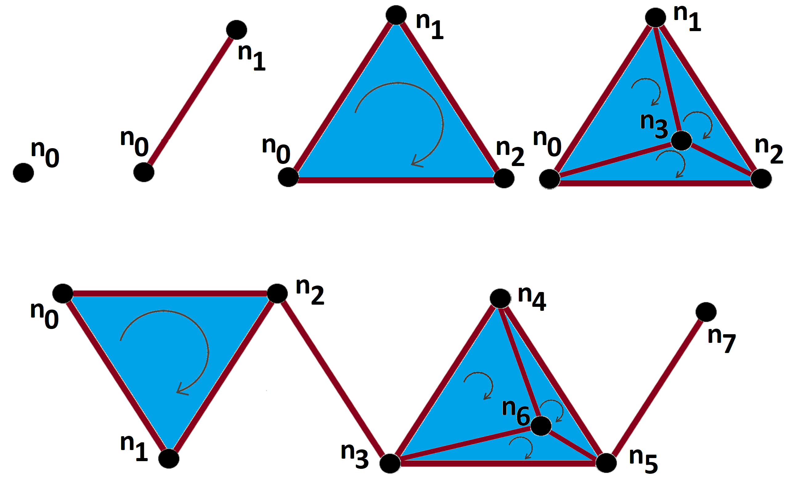
Persistent homology [1, 2, 3, 4] is a technique in TDA for multi-scale analysis of data clouds. In a data cloud, there are no pre-defined links between the points. Therefore, there are no -simplices except -simplices each of which trivially referring to a single data point. Betti numbers are all zero, except which is equal to the number of data points. The main idea of persistent homology is to define an -distance around each data points and then connect those points with overlapping -distances. We may change in the range of . Setting , there will be no link between the points. However, increasing gradually, some points will get connected. When is large enough, (), all data points are connected to each other— i.e. data points will consist an -simplex. In the way to increase from to , number of connected components will change. Also, many loops in the data may appear and disappear—i.e., Betti numbers are changing. On a data cloud, changes in Betti numbers are captured by persistent homology. More precisely, Persistence Diagram [1] captures the birth and death ’s of each component, loop, void, etc. An example for persistent homology on a data cloud along with the resulted persistence diagram are illustrated in Fig. 3. Alternatively, we may show the birth and the death of loops with barcodes where each hole is represented by a bar from its birth to its death [5, 6, 7]. For a more general review of persistent homology and its applications we refer the reader to [3, 8, 9, 10].
While TDA and specially persistent homology are applied on a wide range of problems (e.g., system analysis [11, 12, 13, 14, 15, 16], network coverage [17, 18], etc), there are only a few studies using them for natural language processing. Zhu in [19] used persistent homology to find repetitive patterns in the text, comparing vector space representations of different blocks in the documents. Doshi and Zadrozny in [20] utilized Zhu’s algorithm [19] for movie genre detection on the IMDB data set of movie plot summaries. The authors showed how persistent homology can improve the classification. In [21], Wagner et al. utilized TDA to measure the discrepancy among documents represented by their TF-IDF matrices. Guan et al. in [22] utilized topological collapsing algorithm [23] to develop an unsupervised method of key-phrase extraction. Almgren et al. in [24] and [25] examined the feasibility of persistent homology for social network analysis. The authors utilized Mapper algorithm [26] to predict image popularity based on word embedding representations of images’ captions. In [27], Torres-Tramón et al. introduced a topic detection algorithm for Twitter data analysis utilizing Mapper algorithm to map the term frequency matrix to the topological representations. Savle and Zardozny in [28] used TDA to study discourse structures and showed that topological features derived from the relation of sentences can be informative for prediction of text entailment. Considering the word embedding representation of the text as high-dimensional time-series, some ideas from the recent applications of persistent homology in time series analysis [13, 14, 15, 11, 16] are also considerable for text processing.


In our prior work [29], we applied persistent homology on a set of novels and tried to predict the author without using any conventional text mining features. For each novel, we built an adjacency matrix whose elements are measuring the co-appearance of the main characters (persons) in the novel. Utilizing persistent homology, we analyzed on the graph of the main characters in the novels and fed the resulted topological features (conveying topological styles of novelists) to a classifier. Despite the novelty of the algorithm (using persistent homology instead of utilizing conventional text mining features), it is not easily applicable to the general text classification problem. Here, we introduce a different approach using word embeddings and persistent homology which can be applied to the general text classification tasks.
2 Methodology
In our algorithm, Topological Inference of the Embedding Space (TIES) we utilize word embedding and persistent homology. The input is the textual document and the output is a topological representation of the same document. Later we may use these representations for text classification, clustering, etc. Step-by-step specifications of TIES are explained is this section.
2.1 Pre-processing
Like any other text mining method, standard pre-processing possibly including lemmatization, removing stop words and if necessary lowercasing will be applied to the text. Also, there might be some specific pre-processing tasks that are inspired by TDA algorithms.
2.2 Word Embedding Representation
In a document of size , replacing each token with its embedding vector of size will result in a matrix of size . This matrix can naturally be viewed as a -dimensional time series that represents the document. More precisely, each column () will represent the document in dimension of the embedding.
2.3 Aggregation on Sliding Window
One of the easiest and potentially most efficient ways of such smoothing is to replace each element () in with a local average in its neighborhood. Equivalently, we may describe it by taking the summation in the sliding window of size , where so the smoothed vector is
and is the smoothed -dimensional time series that represents the document. For long documents this is almost the same as using a smoother matrix , i.e.,
where is a tridiagonal (for ), pentadiagonal (for ) or heptadiagonal (for ) binary matrix. The only difference is that in the latter definition, no value of time series will be dropped, so the result is only slightly different in size, assuming . Note that we can also use exponential weights in summation of elements in the sliding window instead of simply adding them up. In one of our experiments, we tried the exponential form of:
2.4 Computing Distances
Assume that in a documents, some of the embedding dimensions— and the relation among different dimensions are carrying some information regarding the document. Such information could be revealed in a coordinate system, where each embedding dimension is represented by a data point, and the distance between two data points (embedding dimensions) represents their relation. A possible choice of distance is formulated in Equation 1.
| (1) |
The intuition behind the way of defining distance in Equation 1 is to (1) consider the relation between and via Cosine similarity, (2) distinguish significant embedding dimensions (the term will do this), and (3) make the distance almost non-sensitive to the size of document via term . Note that Equation 1 can be replaced by any other definition satisfying these three conditions. Aggregation on sliding window along with a distance formula like Equation 1 guarantee that the order of the tokens in documents is considered in the final distance matrix , defined by
For simplicity let’s fix , so remembering that each column of as a simple time series is a function of time (the index of word/token in the document),
and assuming that the length of document is large enough () we have
as , so
since shifting the time index will only exclude elements from the beginning or the end of time series and its effect is negligible when . It is easy to show that
and similarly, in a general form for any window size , Equation 2 holds.
| (2) |
Such coefficients will guarantee that the order is considered in the final distance matrix . It means that each embedding dimension for each token in the text is being compared with all the other embedding dimensions in the same token, a few tokens before that, and a few tokens after that, though these comparisons will have different weights. Note that similar equations can be easily derived for correlation-based and covariance-based distances. In any case, the distance matrix is sensitive to the window size , or more generally to the smoothing algorithm. For instance, using exponential smoothing will result in geometric sequence of coefficients instead of arithmetic sequence of coefficients in Equation 2 (i.e., , , ,). Regarding using the sliding window, the choice of is a trade-off between increasing the captured information on one side and decreasing the noise on the other side.
2.5 Applying Persistent Homology
Having the distance matrix for each document, a persistence diagram can be constructed for topological dimension11 1 These dimensions should not be mistaken with embedding dimensions. (number of clusters) and dimension (number of loops) denoted by and respectively. However, this persistence diagram alone is not very useful as the representation of the document.
In our prior work [29] the resulted graph of the main characters (persons) in each novel, and therefore the distance matrix was not annotated nor was needed to be annotated, since we had designed the algorithm to deal with the main characters whatever their names are. In other word, to capture the topological signature of a novelist, it did not matter whether the names of the main characters are shifted. But here, dealing with time-series in different dimensions, the order of embedding dimensions is meaningful, since different embedding dimensions have different roles in representing document. Therefore, feeding the time series to the persistent homology algorithm is meaningless, unless we somehow manage to distinguish different dimensions. One intuitive way is comparing the persistence diagram with and without each embedding dimension. In other word we can measure the change in persistence diagram when we exclude one embedding dimension. We measure the sensitivity of the persistence diagram generated by Ripser [30, 31] to each embedding dimension to use it later as a measure of the sensitivity of the document itself to each embedding dimension. This way the document will be represented in an array of size array of based on and another array of size based on , as formulated in Equation 3, where is any measure of distance between two persistence diagram, e.g, Wasserstein distance.
| (3) |
A block diagram of TIES is shown in Fig. 4.

3 Data Specification
To examine our topological algorithm (TIES), we use the following data sets and predict the labels in multi-class multi labeling classification.
- •
arXiv Papers: We downloaded all of arXiv papers in quantitative finance22 2 https://arXiv.org/archive/q-fin published between 2011 and 2018. Then we selected five major categories (subject tags): “q-fin.GN” (General Finance), “q-fin.ST” (Statistical Finance), “q-fin.MF” (Mathematical Finance), “q-fin.PR” (Pricing of Securities), and “q-fin.RM” (Risk Management). For pre-processing we removed the titles, author names and affiliations, abstracts, keywords and references. Then we tried to predict the subjects solely based on the paper body.
- •
IMDB Movie Review [32]: Using IMDB reviews annotated by positive/negative label, we examined TIES for binary sentiment classification task.
Table 1 contains the specifications of both data sets. Note that each records in the arXiv data set may have more that one label. The histogram of number of labels for each record is shown in Fig. 5. As shown in the histogram, the majority of records in arXiv data set are tagged with only a single label.
| Specification | arXiv Quant. Fin. Papers | IMDB Movie Reviews |
|---|---|---|
| Labels | 5 (Multi-label) | 2 |
| Clean Records | 4601 | 6000 |
| Length of Records | ||
| Frequency of Labels |

In practice, for many of the classification and clustering tasks in text processing, the data covers only very short documents (e.g., a limited data set of social media posts). Therefore a big challenge is training word embedding models on short documents. Such a challenge is beyond the scope of this study and we will use pre-trained versions of word embeddings that are previously trained on large corpora. Specifically, we use the following pre-trained models.
- •
GloVe [33] pre-trained on Wikipedia 2014 and Gigaword 5 with vocabulary size of K and d vectors33 3 http://nlp.stanford.edu/data/glove.6B.zip.
- •
- •
ConceptNet Numberbatch [36] with the vocabulary size of K and d vectors55 5 https://conceptnet.s3.amazonaws.com/downloads/2017/numberbatch/numberbatch-en-17.06.txt.gz.
| Model | Embedding | Window | Prec. | Rec. | F1 | Acc. |
|---|---|---|---|---|---|---|
| TIES + XGBoost | fastText | 3 | 61.9 | 55.4 | 0.575 | 80.1 |
| TIES + XGBoost | GloVe | 3 | 63.1 | 56.7 | 0.597 | 80.7 |
| TIES + XGBoost | Numberbatch | 3 | 68.7 | 60.5 | 0.643 | 82.6 |
| TIES + XGBoost | fastText | 5 | 60.8 | 54.7 | 0.576 | 79.8 |
| TIES + XGBoost | GloVe | 5 | 61.8 | 56.1 | 0.588 | 80.3 |
| TIES + XGBoost | Numberbatch | 5 | 65.5 | 58.4 | 0.617 | 81.6 |
| TIES + XGBoost | fastText | 7 | 58.9 | 54.4 | 0.566 | 79.5 |
| TIES + XGBoost | GloVe | 7 | 62.8 | 56.4 | 0.594 | 80.6 |
| TIES + XGBoost | Numberbatch | 7 | 65.7 | 57.7 | 0.614 | 81.3 |
| TIES + XGBoost | fastText | 7 expon. | 60.3 | 54.6 | 0.573 | 79.7 |
| TIES + XGBoost | GloVe | 7 expon. | 61.2 | 55.9 | 0.584 | 80.2 |
| TIES + XGBoost | Numberbatch | 7 expon. | 66.4 | 59.6 | 0.628 | 82.2 |
| CNN | fastText | - | 57.1 | 64.3 | 60.5 | 80.0 |
| CNN | GloVe | - | 57.6 | 64.2 | 60.7 | 80.6 |
| CNN | Numberbatch | - | 55.0 | 67.6 | 60.7 | 79.8 |
| Model | Embedding | Window | Prec. | Rec. | F1 | Acc. |
|---|---|---|---|---|---|---|
| TIES + XGBoost | fastText | 3 | 84.8 | 85.8 | 0.853 | 85.4 |
| TIES + XGBoost | GloVe | 3 | 86.9 | 88.0 | 0.874 | 87.5 |
| TIES + XGBoost | Numberbatch | 3 | 87.9 | 89.0 | 0.884 | 88.5 |
| TIES + XGBoost | fastText | 5 | 84.2 | 85.2 | 0.847 | 84.8 |
| TIES + XGBoost | GloVe | 5 | 85.6 | 86.6 | 0.861 | 86.2 |
| TIES + XGBoost | Numberbatch | 5 | 86.5 | 87.6 | 0.870 | 87.1 |
| TIES + XGBoost | fastText | 7 | 82.8 | 83.8 | 0.833 | 83.4 |
| TIES + XGBoost | GloVe | 7 | 83.8 | 84.8 | 0.843 | 84.4 |
| TIES + XGBoost | Numberbatch | 7 | 85.3 | 86.3 | 0.858 | 85.9 |
| TIES + XGBoost | fastText | 7 expon. | 84.3 | 85.3 | 0.848 | 84.9 |
| TIES + XGBoost | GloVe | 7 expon. | 86.5 | 87.6 | 0.870 | 87.1 |
| TIES + XGBoost | Numberbatch | 7 expon. | 87.0 | 88.1 | 0.875 | 87.6 |
| Shauket et al. (2020) [37] | Lexicon based | - | 86.7 | |||
| Giatsoglou et al. (2017) [38] | Hybrid | - | 0.880 | 87.8 |
| Subject | Test Records | Precision | Recall | F1 | Accuracy |
|---|---|---|---|---|---|
| q-fin.GN | 410 | 73.2 | 68.5 | 0.708 | 83.8 |
| q-fin.ST | 396 | 70.2 | 67.5 | 0.688 | 83.6 |
| q-fin.MF | 306 | 66.0 | 45.6 | 0.539 | 77.5 |
| q-fin.PR | 305 | 69.5 | 55.2 | 0.615 | 82.7 |
| q-fin.RM | 307 | 62.5 | 61.0 | 0.617 | 84.5 |
4 Results and Discussion
We run our binary classification and multi-label multi-class classification on both data set using XGBoost [39, 40] with the parameters , , , and . In each data set 2/3 of the records were randomly selected for training and 1/3 used for testing. Table 2 and Table 3 show the results on arXiv paper data set and IMBD movie review data set, respectively. On each data set, we run the classifier using different pre-trained embedding models and different sliding window sizes to smooth the embedding signals. For both arXiv papers set and IMDB Movie Review data set, the best result is achieved using ConceptNet Numberbatch as pre-trained embedding and window size of . Detailed results for arXiv papers set are shown in Table 4.
To evaluate out results, for arXiv data set we run a convolutional neural network using the same pre-trained word embeddings. As shown in Table 2, our best configuration using TIES outperforms the base CNN model in terms of accuracy and F1 score. For IMDB reviews data set, we compare our results to the previous results of Shauket et al. (2020) [37] lexicon based approach and Giatsoglou et al. (2017) [38] hybrid approach. The comparison reveals that TIES outperforms the previous models.
5 Conclusion
In this paper, we introduced a novel method to define and extract topological features from word embedding representations of corpus and used them for text classification. We utilized persistent homology, the most commonly tool from topological data analysis to interpret the embedding space of each textual documents. In our experiments, we showed that working on textual documents, our defined topological features can outperform conventional text mining features. Specially when the textual documents are long, using these topological features can improve the results. However, in TIES, we are analyzing different embedding dimensions as time series. Thus, to achieve reasonable results, a large number of tokens in each textual document is required. We acknowledge this issue as the main limitation of our algorithm. Also, it is not easy to measure and/or interpret the impact of different parts of the text input on the output in TIES. This is one of the possible future directions for this study.
References
- [1] Herbert Edelsbrunner, David Letscher, and Afra Zomorodian. Topological persistence and simplification. In Foundations of Computer Science, 2000. Proceedings. 41st Annual Symposium on, pages 454–463. IEEE, 2000.
- [2] Gunnar Carlsson. Topology and data. Bulletin of the American Mathematical Society, 46(2):255–308, 2009.
- [3] Herbert Edelsbrunner and John Harer. Persistent homology-a survey. Contemporary mathematics, 453:257–282, 2008.
- [4] Li M Chen, Zhixun Su, and Bo Jiang. Mathematical Problems in Data Science. Springer, 2015.
- [5] Anne Collins, Afra Zomorodian, Gunnar Carlsson, and Leonidas J Guibas. A barcode shape descriptor for curve point cloud data. Computers & Graphics, 28(6):881–894, 2004.
- [6] Gunnar Carlsson, Afra Zomorodian, Anne Collins, and Leonidas J Guibas. Persistence barcodes for shapes. International Journal of Shape Modeling, 11(02):149–187, 2005.
- [7] Robert Ghrist. Barcodes: the persistent topology of data. Bulletin of the American Mathematical Society, 45(1):61–75, 2008.
- [8] Afra Zomorodian and Gunnar Carlsson. Computing persistent homology. Discrete & Computational Geometry, 33(2):249–274, 2005.
- [9] Elizabeth Munch. A user’s guide to topological data analysis. Journal of Learning Analytics, 4(2):47–61, 2017.
- [10] Shafie Gholizadeh and Wlodek Zadrozny. A short survey of topological data analysis in time series and systems analysis. arXiv preprint arXiv:1809.10745, 2018.
- [11] Slobodan Maletić, Yi Zhao, and Milan Rajković. Persistent topological features of dynamical systems. Chaos: An Interdisciplinary Journal of Nonlinear Science, 26(5):053105, 2016.
- [12] Joshua Garland, Elizabeth Bradley, and James D Meiss. Exploring the topology of dynamical reconstructions. Physica D: Nonlinear Phenomena, 334:49–59, 2016.
- [13] Cássio MM Pereira and Rodrigo F de Mello. Persistent homology for time series and spatial data clustering. Expert Systems with Applications, 42(15-16):6026–6038, 2015.
- [14] Firas A Khasawneh and Elizabeth Munch. Stability determination in turning using persistent homology and time series analysis. In ASME 2014 International Mechanical Engineering Congress and Exposition, pages V04BT04A038–V04BT04A038. American Society of Mechanical Engineers, 2014.
- [15] Jose A Perea and John Harer. Sliding windows and persistence: An application of topological methods to signal analysis. Foundations of Computational Mathematics, 15(3):799–838, 2015.
- [16] Bernadette J Stolz, Heather A Harrington, and Mason A Porter. Persistent homology of time-dependent functional networks constructed from coupled time series. Chaos: An Interdisciplinary Journal of Nonlinear Science, 27(4):047410, 2017.
- [17] Vin De Silva and Robert Ghrist. Coordinate-free coverage in sensor networks with controlled boundaries via homology. The International Journal of Robotics Research, 25(12):1205–1222, 2006.
- [18] Vin De Silva, Robert Ghrist, et al. Coverage in sensor networks via persistent homology. Algebraic & Geometric Topology, 7(1):339–358, 2007.
- [19] Xiaojin Zhu. Persistent homology: An introduction and a new text representation for natural language processing. In IJCAI, pages 1953–1959, 2013.
- [20] Pratik Doshi and Wlodek Zadrozny. Movie genre detection using topological data analysis. In International Conference on Statistical Language and Speech Processing, pages 117–128. Springer, 2018.
- [21] Hubert Wagner, Paweł Dłotko, and Marian Mrozek. Computational topology in text mining. In Computational Topology in Image Context, pages 68–78. Springer, 2012.
- [22] Hui Guan, Wen Tang, Hamid Krim, James Keiser, Andrew Rindos, and Radmila Sazdanovic. A topological collapse for document summarization. In Signal Processing Advances in Wireless Communications (SPAWC), 2016 IEEE 17th International Workshop on, pages 1–5. IEEE, 2016.
- [23] Adam C Wilkerson, Terrence J Moore, Ananthram Swami, and Hamid Krim. Simplifying the homology of networks via strong collapses. In Acoustics, Speech and Signal Processing (ICASSP), 2013 IEEE International Conference on, pages 5258–5262. IEEE, 2013.
- [24] Khaled Almgren, Minkyu Kim, and Jeongkyu Lee. Mining social media data using topological data analysis. In Information Reuse and Integration (IRI), 2017 IEEE International Conference on, pages 144–153. IEEE, 2017.
- [25] Khaled Almgren, Minkyu Kim, and Jeongkyu Lee. Extracting knowledge from the geometric shape of social network data using topological data analysis. Entropy, 19(7):360, 2017.
- [26] Gurjeet Singh, Facundo Mémoli, and Gunnar E Carlsson. Topological methods for the analysis of high dimensional data sets and 3d object recognition. In SPBG, pages 91–100, 2007.
- [27] Pablo Torres-Tramón, Hugo Hromic, and Bahareh Rahmanzadeh Heravi. Topic detection in twitter using topology data analysis. In International Conference on Web Engineering, pages 186–197. Springer, 2015.
- [28] Ketki Savle, Wlodek Zadrozny, and Minwoo Lee. Topological data analysis for discourse semantics? In Proceedings of the 13th International Conference on Computational Semantics-Student Papers, pages 34–43, 2019.
- [29] Shafie Gholizadeh, Armin Seyeditabari, and Wlodek Zadrozny. Topological signature of 19th century novelists: Persistent homology in text mining. Big Data and Cognitive Computing, 2(4):33, 2018.
- [30] Ulrich Bauer. Ripser: efficient computation of vietoris-rips persistence barcodes. arXiv preprint arXiv:1908.02518, 2019.
- [31] Ulrich Bauer. Ripser: a lean c++ code for the computation of vietoris–rips persistence barcodes. Software available at https://github. com/Ripser/ripser, 2017.
- [32] Andrew L Maas, Raymond E Daly, Peter T Pham, Dan Huang, Andrew Y Ng, and Christopher Potts. Learning word vectors for sentiment analysis. In Proceedings of the 49th annual meeting of the association for computational linguistics: Human language technologies-volume 1, pages 142–150. Association for Computational Linguistics, 2011.
- [33] Jeffrey Pennington, Richard Socher, and Christopher Manning. Glove: Global vectors for word representation. In Proceedings of the 2014 conference on empirical methods in natural language processing (EMNLP), pages 1532–1543, 2014.
- [34] Piotr Bojanowski, Edouard Grave, Armand Joulin, and Tomas Mikolov. Enriching word vectors with subword information. arXiv preprint arXiv:1607.04606, 2016.
- [35] Armand Joulin, Edouard Grave, Piotr Bojanowski, and Tomas Mikolov. Bag of tricks for efficient text classification. arXiv preprint arXiv:1607.01759, 2016.
- [36] Robert Speer, Joshua Chin, and Catherine Havasi. Conceptnet 5.5: An open multilingual graph of general knowledge. In Thirty-First AAAI Conference on Artificial Intelligence, 2017.
- [37] Zeeshan Shaukat, Abdul Ahad Zulfiqar, Chuangbai Xiao, Muhammad Azeem, and Tariq Mahmood. Sentiment analysis on imdb using lexicon and neural networks. SN Applied Sciences, 2(2):1–10, 2020.
- [38] Maria Giatsoglou, Manolis G Vozalis, Konstantinos Diamantaras, Athena Vakali, George Sarigiannidis, and Konstantinos Ch Chatzisavvas. Sentiment analysis leveraging emotions and word embeddings. Expert Systems with Applications, 69:214–224, 2017.
- [39] Tianqi Chen, Tong He, Michael Benesty, Vadim Khotilovich, and Yuan Tang. Xgboost: extreme gradient boosting. R package version 0.4-2, pages 1–4, 2015.
- [40] Tianqi Chen and Carlos Guestrin. Xgboost: A scalable tree boosting system. In Proceedings of the 22nd acm sigkdd international conference on knowledge discovery and data mining, pages 785–794. ACM, 2016.