Information geometry for phylogenetic trees

For $N=2,3,\ldots$ we define $U_{\!N}$ to be the set of unrooted phylogenetic trees on $N$ taxa. More specifically, a tree $T$ is an element of $U_{\!N}$ if it satisfies the following conditions. First, $T$ contains exactly $N$ vertices with degree 1, which are called leaves, and these are bijectively labelled $1,\ldots,N$. Secondly, $T$ must contain no vertices with degree $2$. Thirdly, each edge $e$ in $T$ is assigned a length $\ell^{e}\geq 0$ with $\ell^{e}\neq 0$ if $e$ contains a leaf. An edge in a tree is called a pendant edge if it contains a leaf; otherwise it is called an internal edge. Similarly, the vertices which are not leaves are called internal vertices.

The edge lengths $\ell^{e}$ on any given tree $T\in U_{\!N}$ define a path length distance between any pair of leaves. The path length on $T$ between $u,v\in\{1,\ldots,N\}$ will be denoted $\ell_{uv}$.

Each tree $T\in U_{\!N}$ contains at most $2N-3$ edges, in which case the tree is called fully resolved or bifurcating, and all internal vertices have degree $3$. Trees with fewer edges are called unresolved, and for $N>3$, these contain at least one vertex with degree $4$ or more. Trees which contain only the $N$ pendant edges joined at a single degree-$N$ internal vertex are called star trees.

A tree $T$ is rooted when some internal point $\rho\in T$ is labelled as being the root. This is conveniently achieved by adding an additional taxon labelled $0$ to the tree via a pendant edge of length zero. It follows that the set of rooted phylogenetic trees satisfies the same conditions as $U_{\!N}$, except the leaves are bijectively labelled $0,1,\ldots,N$, and the pendant edge containing taxon $0$ has zero length. We will work with unrooted trees, but our results are easily transferred to the space of rooted trees via this relationship.

Every fully resolved tree will correspond to a fully resolved BHV-tree (reviewed in Section 2.2) and to a fully resolved wald, as introduced below in Section 2.4. In both BHV tree space and in wald space, unresolved trees will be identified with other trees with certain internal edges having zero length, so that conceptually a missing edge is the same as a zero length edge.

Billera et al. 2001 defined a space of phylogenetic trees, subsequently known as BHV tree space, and described its geometry. BHV tree space can be described via an embedding in $\mathbb{R}^{d}$ for dimension $d$ which increases exponentially with the number of leaves. However, we have chosen to describe BHV tree space in a way different from the original authors, and we define it as a quotient space. As a result, the wald space introduced in the next section is a superset of BHV tree space when the spaces are regarded simply as sets, clarifying the relationship between the two spaces. Importantly, we allow internal edges on trees to have length zero, and under the quotient these are equivalent to trees with those edges missing. A second difference is that while Billera et al. 2001 worked with rooted trees, we work with unrooted trees. As described in Section 2.3, the distribution on binary characters determined by a tree does not depend on the root position under the two-state symmetric model, and so unrooted trees are more natural to work with.

BHV tree space is defined using the notion of splits, where a split is a bipartition of the leaf labels $1,\ldots,N$ into two disjoint sets. Cutting an edge of a tree induces such a bipartition of the leaves, and so each edge on a tree corresponds to a split, and the terms split and edge can be used interchangeably. The set of splits represented by a tree is called its topology.

Arbitrary sets of splits do not typically determine valid tree topologies: the splits of a tree must satisfy a compatibility condition. For example, the splits $\{1,2\},\{3,4,\ldots,N\}$ and $\{1,3\},\{2,4,\ldots,N\}$ are incompatible, since leaf $1$ cannot be grouped next to both $2$ and $3$ on the same tree. For any topology $\tau$ with $k$ internal edges, $0\leq k\leq N-3$, the set of trees in $U_{\!N}$ with that topology is bijectively parametrized by $\mathbb{R}_{>0}^{N}\times\mathcal{O}_{\tau}$ where the first term in the product parametrizes the pendant edge lengths that, by definition, are strictly positive, and $\mathcal{O}_{\tau}=\mathbb{R}^{k}_{\geq 0}$ parametrizes the internal edge lengths.

The set $\mathcal{O}_{\tau}$ is called the orthant associated with topology $\tau$, and we identify the set of all trees with topology $\tau$ with $\mathbb{R}_{>0}^{N}\times\mathcal{O}_{\tau}$. Under this identification, the set of all trees $U_{\!N}$, as defined in Section 2.1, is the disjoint union

where the disjoint union is taken over all possible topologies $\tau$.

The unrooted BHV tree space $\mathcal{U}_{N}$ is obtained by taking the quotient of $U_{\!N}$ with respect to an equivalence relation:

Two trees in $U_{\!N}$ are equivalent under $\sim$ if and only if they are identical modulo the presence of internal splits with zero length, as shown in Figure 1. The quotient space factorizes as

where the first term parametrizes the lengths of the pendant edges and the space $\mathrm{BHV}_{\!N}$ parametrizes the topology and internal edge lengths of the BHV-trees. When $\tau$ is fully resolved, $\mathcal{O}_{\tau}$ is called a maximal orthant. Unresolved trees correspond to points on the boundaries of maximal orthants; they can be obtained from fully resolved trees by shrinking internal edge lengths down to zero.

Since there are $(2N-5)!!$ fully resolved unrooted topologies, $\mathrm{BHV}_{\!N}$ can be thought of as being constructed by gluing this number of maximal orthants together along their boundaries, where two points are identified if they correspond to the same tree. For example, when $N=4$, there are three fully resolved topologies, each of which contains a single internal edge. The space $\mathrm{BHV}_{\!4}$ therefore consists of three copies of $\mathbb{R}_{\geq 0}$ glued together at the origin. The origin corresponds to the star trees, while the location along each of the three copies of $\mathbb{R}_{\geq 0}$ gives the length of the internal edge in each of the three possible fully resolved topologies. For $N=5$ there are $15$ possible unrooted tree topologies, each of which contains two internal edges. It follows that $\mathrm{BHV}_{\!5}$ consists of $15$ copies of $\mathbb{R}^{2}_{\geq 0}$ glued along their boundaries. At each codimension-1 boundary, three maximal orthants are joined together. This is because when a single internal edge is contracted to length zero, a degree 4 vertex is obtained, and there are 3 possible ways to add in an edge, including the original edge, in order to obtain a fully resolved topology, as illustrated by Figure 2.

The metric on $\mathrm{BHV}_{\!N}$ is constructed as follows. The basic idea is that for trees with the same fully-resolved topology but different vectors of internal edge lengths, say $\boldsymbol{\ell}_{1}$ and $\boldsymbol{\ell}_{2}$, the distance is the Euclidean distance $\|\boldsymbol{\ell}_{1}-\boldsymbol{\ell}_{2}\|$, and the corresponding geodesic is the straight line segment in the orthant containing the trees. Billera et al. 2001 showed that there exists a unique shortest path between any two points in $\mathrm{BHV}_{\!N}$, for which path length is measured using the Euclidean distance in each orthant, and the length of these defines a metric on $\mathrm{BHV}_{\!N}$ which we denote $d_{\mathrm{BHV}}$. A metric on $\mathcal{U}_{N}$, denoted $d_{\mathcal{U}_{N}}$, is obtained as the product metric when the metric on pendant edges is taken to be the Euclidean distance. An algorithm has been developed which constructs geodesics and calculates their lengths in $O(N^{4})$ time (Owen and Provan 2011).

Genetic sequence evolution is typically modelled using discrete-valued continuous-time Markov processes defined over the edges of a tree $T$ (Yang 2006; Bryant et al. 2005). DNA sequence evolution is modelled by associating to each point $t\in T$, a random variable $X(t)$ which takes values in an alphabet $\{A,C,G,T\}$. In this paper, however, we will consider the two-state symmetric Markov process with alphabet $\Omega=\{0,1\}$. This simplification is made in order to make the mathematics more tractable and for computational speed. Nonetheless, some of the calculations using the two-state symmetric can readily be performed using DNA models. More details are given in the thesis of Garba 2019 in which simulations show similarity of geometries obtained from the two- and the four-state process. The transition probability of the symmetric two-state model is defined in terms of the path length $\ell_{t_{1}t_{2}}$ between any two points $t_{1},t_{2}\in T$:

The stationary distribution of this Markov process is $Bern(1/2)$, and the process is assumed to be in its stationary state over the tree. As a result, for all $t\in T$, $X(t)$ has a marginal Bernoulli distribution, $X(t)\sim Bern(1/2)$. While the random variables $X_{1},\ldots,X_{N}$ at the leaves of the tree have the same marginal distributions, they are not independent since the tree imposes a dependence structure. The following lemma determines certain moments of the process $X(t)$ giving insight on the dependence structure of $X_{1},\dots,X_{N}$. The proof is straightforward using the transition probabilities in Equation (1).

It is straightforward to simulate realizations of $X(t)$ in the following way. First simulate a Poisson process with rate 1 independently on each edge of the tree. The positions of the simulated events correspond to points at which $X(t)$ changes parity. Secondly, pick any point $t_{0}\in T$ which is not a change point and sample $X(t_{0})$ from $Bern(1/2)$. The change points generated from the Poisson process then determine the value of $X(t)$ for all other $t\in T$. The distribution obtained is independent of the choice of $t_{0}$, because the Markov process is reversible. In particular, the Markov process is independent of the choice of $t_{0}$, which could be considered as a root.

Under the model, each edge length can be interpreted as the expected number of change points that occur over the edge. Internal edges are allowed to have length zero, which means that no change in $X(t)$ occurs over the edge. On the other hand, when edges are long, the number of changes is likely to be large, and the letters at either end of the edge are weakly correlated. Biologists refer to this effect as saturation. A fixed change of edge length $\delta\ell$ therefore has more effect on the distribution of characters when applied to a short edge as opposed to a long edge in some given tree. For example, an increase of $\delta\ell=0.1$ to an edge with length $\ell=0.1$ approximately doubles the probability that the letters at either end of the edge are different, but the same change to an edge of length $\ell=10$ has almost no effect on this probability, which due to saturation is very close to $1/2$. This idea becomes important when we consider defining distances between trees via the information they represent, in particular using the probability mass function of the nontrivial distribution of $(X_{1},\ldots,X_{N})$.

The following wald space gives an alternative viewpoint of phylogenetic trees by regarding them as Markov models for sequence evolution (Kim 2000; Moulton and Steel 2004; Gill et al. 2008). We will give a description of the wald space that is related to the edge-product space of previous authors, by defining it as a quotient space which adds trees with infinitely long edges to BHV tree space. As described in the introduction, each probabilistic metric considered by Garba et al. 2018 converges to zero in the limit as all the edge lengths in a pair of trees simultaneously tend to infinity. This behaviour indicates that shortest paths might cross a tree with infinitely long edges, which is why we add this boundary at infinity. Furthermore, we allow pendant edges of length zero under certain conditions. Thus, in the wald space, edge lengths $\ell^{e}$ take values in $\mathbb{R}_{\geq 0}\cup\{\infty\}$. It is convenient to reparametrize to the $\boldsymbol{\lambda}$-parametrization by defining weights $\lambda^{e}=1-\exp(-\ell^{e})$, so $\lambda^{e}\in[0,1]$. Under this transformation, $\mathrm{BHV}_{\!N}$ becomes a set of unit cubes, rather than orthants, glued along faces where $\lambda^{e}=0$ for one or more edges. The wald space is defined by imposing additional gluing rules on faces where $\lambda^{e}=1$.

In order to be able to identify trees with infinitely long edges along faces where $\lambda^{e}=1$, we construct the wald space from forests, that is, disjoint unions of unrooted trees. We start with a preliminary space leading to the definition of the wald space further below. Let $W_{N}$ be the collection of forests satisfying the following necessary and sufficient conditions for each $F\in W_{N}$.

1. 1.

   The forest $F$ contains exactly $N$ labelled vertices, these are called leaves and labelled $1,\ldots,N$.

2. 2.

   There are no unlabelled vertices in $F$ of degree 0,1 and 2.

3. 3.

   For every pair of leaves $u,v$ in the same tree in $F$, at least one edge $e$ on the unique path from $u$ to $v$ satisfies $\lambda^{e}>0$.

Clearly, $U_{\!N}\subset W_{N}$. The condition on the edge weights ensures that no pair of leaves is coincident and consequently that metrics are always well-defined, as described in Section 3.2. We impose an equivalence relation $\sim$ on $W_{N}$, defined by the following two rules.

The wald space $\mathcal{W}_{N}$ is defined to be the quotient $W_{N}\big/\sim$ and it immediately follows that as sets $\mathcal{U}_{N}\subset\mathcal{W}_{N}$, but the geometry imposed on $\mathcal{W}_{N}$ will be completely different from the geometry of the BHV space.

The boundary rule at infinity requires some explanation. The rule declares that edges of weight $\lambda^{e}=1$ (or equivalently length $\ell^{e}=\infty$) can be deleted from a forest $F$, but unlike the BHV rule for which the vertices at the ends of the edge are merged, edge removal disconnects a tree in $F$. When resulting degree-2 vertices are removed, the edge length is preserved so that the new edge has length $\ell^{e}+\ell^{\tilde{e}}$. The corresponding weight $\lambda$ is given by $\lambda=1-\exp(-(\ell^{e}+\ell^{\tilde{e}}))=\lambda^{e}+\lambda^{\tilde{e}}-\lambda^{e}\lambda^{\tilde{e}}$. Unlike the BHV boundary rule, in which finitely many trees are identified in each equivalence class, infinitely many combinations of edge weights $\lambda^{e},\lambda^{\tilde{e}}$ give rise to the same value $\lambda^{e}+\lambda^{\tilde{e}}-\lambda^{e}\lambda^{\tilde{e}}$. It follows that an uncountable collection of forests can be identified into a single equivalence class in $\mathcal{W}_{N}$.

In the edge-product space (Moulton and Steel 2004; Gill et al. 2008), an alternative parametrization is used, defining $\mu^{e}=1-\lambda^{e}=\exp(-\ell^{e})$ to be the weight of edge $e$. This parametrization has the advantage that sums of edge lengths $\ell^{1}+\cdots+\ell^{m}$ become products of edge weights $\mu^{1}\times\cdots\times\mu^{m}$ (hence the name ‘edge-product’). The boundary at infinity rule is simpler under this parametrization: the weights in Figure 3 panel (b) become $\mu^{e}$, $\mu^{\tilde{e}}$ and $0$ on the left and $\mu^{e}\mu^{\tilde{e}}$ on the right. However, under the $\boldsymbol{\mu}$-parametrization, the BHV boundary with $\ell^{e}=0$ lies on faces of cubes with $\mu^{e}=1$, whereas the boundary at infinity has $\mu^{e}=0$. We prefer to work with the $\boldsymbol{\lambda}$-parametrization since it gives a more intuitive interpretation of the weights, i.e. $\ell^{e}=0$ corresponds to $\lambda^{e}=0$ and $\ell^{e}=\infty$ corresponds to $\lambda^{e}=1$. Forests which contain more than one connected component lie in the faces of cubes with at least one $\lambda^{e}=1$. Since the pendant edges can be expanded out to infinite length, they are also subject to the boundary at infinity rule, and so the representation of pendant edge lengths in $\mathcal{W}_{N}$ is not via a product geometry, as it is for BHV tree space. While the star trees correspond to all internal edges having zero length, $\mathcal{W}_{N}$ also contains a point which consists of $N$ isolated vertices.

The BHV boundaries enable tree topologies to be changed via nearest neighbour interchange (NNI) operations (as illustrated by Figure 2). The boundary at infinity corresponds to a different topological operation, called tree bisection and reconnection (TBR) (Allen and Steel 2001). Under this operation, an edge $e$ in a tree can be expanded up to the boundary $\lambda^{e}=1$. Removing the edge bisects the tree, and the two components can be reconnected by an edge ${\tilde{e}}$ with $\lambda^{\tilde{e}}=1$ placed arbitrarily between the two trees. Reducing the weight $\lambda^{\tilde{e}}$ down from 1 then gives a tree with a topology different from the original tree. It follows that there exist continuous paths in the wald space between trees with different topologies, which pass through the boundary at infinity and, as a result, change tree topology via TBR operations. This is in contrast to BHV tree space in which paths between trees of different topologies involve only NNI operations, as edges are contracted down to length zero and alternative edges are expanded out.

While the set $\mathcal{W}_{N}$ was defined above via an equivalence relation on forests, we also need to understand how it parametrizes Markov models and then characterise its elements again as probability mass functions on $\{0,1\}^{N}$. The two-state symmetric Markov process extends from being defined on trees to forests by taking the process on each connected component in a forest to be independent of the other components. This defines a distribution $p_{F}$ on $\{0,1\}^{N}$ for each $F\in W_{N}$. In fact the distribution uniquely determines the equivalence class of $F$, and vice versa, as the following lemma shows.

A proof is given in the Appendix.

Note that the forest consisting of $N$ isolated vertices corresponds to the random variables $X_{1},\ldots,X_{N}$ being independent, and this can be obtained from any tree by expanding all edges one after the other, as, by definition, there is at least one edge between any two leaves.

Suppose that $\theta:X\rightarrow Y$ where $(Y,d)$ is a metric space and $\theta$ is injective. We will say that $X$ is embedded in $Y$, and refer to $Y$ as the ambient space. The embedding can be used to construct certain metrics on $X$. First, since $\theta$ is injective, $d$ pulls back to define a metric on $X$ which we denote $d_{X}$:

for all $x_{1},x_{2}\in X$. The pull back metric is often called the induced extrinsic metric and, it is simply the restriction of $d$ to $X\subseteq Y$, and so when the context is clear, it is also denoted $d$. The probabilistic metrics described in Section 3.2 are constructed in this way. A second metric, called the induced intrinsic metric and denoted $d^{*}(x_{1},x_{2})$, is defined as the infimum of the length of all possible paths in $X$ between $x_{1},x_{2}\in X\subseteq Y$ when path length is measured using the metric $d$. If no path with finite length exists between $x_{1}$ and $x_{2}$ then $d^{*}(x_{1},x_{2})=\infty$, in which case $d^{*}$ is not a metric. Details of this construction of the induced intrinsic metric are given by Bridson and Haefliger 2011. The metrics $d$ and $d^{*}$, if well-defined, give $X$ the structure of a length space, which is a space in which the metric between points $x_{1},x_{2}$ is the infimum of the lengths of paths between those points. Length spaces are similar to geodesic metric spaces, except that the infimum is not necessarily achieved by a path lying within the space; in a geodesic metric space a minimum length path exists between every pair of points, and so every geodesic metric space is a length space. An example of a length space which is not a geodesic metric space is $\mathbb{R}^{2}$ with the origin removed and the Euclidean metric. Points antipodal to the origin cannot be joined by a geodesic, but the distance between them is the infimum of the lengths of paths joining the points.

In order to illustrate the relationship between $d$ and $d^{*}$, consider the example of the embedding of the unit sphere $X=S^{2}$ in $Y=\mathbb{R}^{3}$ equipped with the Euclidean metric $d$. For any two points $x_{1},x_{2}$, $d(x_{1},x_{2})$ is the length of the straight line segment in the ambient space $\mathbb{R}^{3}$ joining the points. This metric is usually called the chordal metric on $S^{2}$. However, when we consider paths between $x_{1},x_{2}$ which are restricted to lie in $S^{2}$, the shortest paths (with respect to $d$) are great circles, and the induced metric $d^{*}$ is the arc length metric. In fact, $S^{2}$ is a geodesic metric space, since the infimum of path length is always achieved by a great circle.

In the following Section 3.2, the wald space $\mathcal{W}_{N}$ will be embedded in the space of distributions of characters. Later in Section 4 it will be embedded in the space of $N\times N$ symmetric positive definite matrices. Each embedding will be used to construct metrics on $\mathcal{W}_{N}$.

Here we briefly describe the probabilistic metrics developed by Garba et al. 2018 since these will be used for comparison with other metrics. The Kullback-Leibler divergence is a commonly used measure of the difference between two distributions. Given two probability mass functions $p,q$ on characters $\{0,1\}^{N}$, the Kullback-Leibler divergence from $q$ to $p$ is defined as

provided $p(s)=0$ only when $q(s)=0$. The Kullback-Leibler divergence is not a metric since it is not symmetric. However, metrics can be defined as follows: the Jensen-Shannon metric $d_{JS}$ is defined by

and the Hellinger metric $d_{H}$ is defined by

Recently, probabilistic metrics have been developed which are based on distributions of gene trees instead of distributions of characters (Adams and Castoe 2019).

The Kullback-Leibler divergence, squared Jensen-Shannon metric and squared Hellinger metric are all examples of a more general class of distances between probability distributions known as $f$-divergences. Given any convex function $f(t)$ such that $f(1)=0$, the $f$-divergence of $p$ from $q$ is defined as

The Kullback-Leibler divergence $D_{KL}(p;q)$ is obtained by taking $f(t)=t\log t$, while the reversed divergence $D_{KL}(q;p)$ is obtained with $f(t)=-\log(t)$. The squared Jensen-Shannon metric and squared Hellinger metric can also be obtained by using more complicated functions $f$, cf. Sason and Verdu 2016.

Now, let $F\in W_{N}$ be a forest representative of a wald $[F]\in\mathcal{W}_{N}$. As described in Section 2.4, the distributions at leaves of different trees of $F$ are independent. For two leaves in the same tree in $F$, some degree of evolution occurs between them since by definition of $W_{N}$ no two leaves are coincident. Therefore, all characters are possible, giving

It follows that the Kullback-Leibler divergence is always well-defined between distributions of characters corresponding to forest representatives from the wald space. Since by Lemma 2.3 the map $[F]\mapsto p_{F}$ is injective for $[F]\in\mathcal{W}_{N}$ the Jensen-Shannon and Hellinger metrics pull back to define extrinsic metrics on the wald space $\mathcal{W}_{N}$ (analogously to (Garba et al. 2018)). As already mentioned in the introduction, statistical methods rely heavily on the intrinsic nature of metrics, and thus we aim for more geometrical structure in the next section by imposing the Fisher information metric (a Riemannian metric) onto the wald space.

BHV tree space $\mathcal{U}_{N}$ and wald space $\mathcal{W}_{N}$ both do not have the structure of a manifold globally, but the interior of each maximal orthant is a manifold parametrized by $\boldsymbol{\ell}$ or $\boldsymbol{\lambda}$. Therefore we consider first the information geometry on the subspaces of wald space corresponding to a fixed fully resolved tree topology – here every wald has only one single tree representative, since every wald corresponding to a forest with more than one component, as well as a wald containing a pendant edge with length zero, lies on the boundary of unit cubes corresponding to fully resolved tree topologies. Secondly, we establish global results about the constructed geometry of $\mathcal{W}_{N}$.

Thus suppose $\tau$ is a fully resolved tree topology, and that trees with this topology are parametrized by $\boldsymbol{\ell}=(\ell^{1},\ldots,\ell^{2N-3})\in\mathbb{R}_{>0}^{N}\times\mathcal{O}_{\tau}$. Let $p_{\boldsymbol{\ell}}(s)$ be the probability mass function $p_{T}(s)$ associated with tree $T$ determined by $\tau,\boldsymbol{\ell}$. Recalling that $p_{\boldsymbol{\ell}}(s)>0$ for all $s$, due to (3), the Fisher information matrix at $\boldsymbol{\ell}$ is

for $i,j=1,\ldots,2N-3$ where $\partial_{i}=\partial/\partial_{\ell^{i}}$. This defines a Riemannian inner product on the tangent space of $\mathbb{R}_{>0}^{N}\times\mathcal{O}_{\tau}$ at $\boldsymbol{\ell}$ (that is a copy of $\mathbb{R}^{2N-3}$) which gives a way to measure the lengths of paths. Specifically, if $p_{\boldsymbol{\ell}}$ and $p_{\boldsymbol{\ell}+\delta\boldsymbol{\ell}}$ lie infinitesimally close on a path, then the squared path length between them is defined to be $\sum_{i,j}\delta\ell^{i}g_{ij}(\boldsymbol{\ell})\delta\ell^{j}$. Standard results from Riemannian differential geometry show that if $\boldsymbol{\ell}(t)$ is a path in $\mathbb{R}_{>0}^{N}\times\mathcal{O}_{\tau}$ then it is locally a geodesic (i.e. it minimizes path length) if it satisfies the differential equation

where $\Gamma_{ij}^{k}(\boldsymbol{\ell})$ are the Christoffel symbols

The matrix $g^{ij}$ is the inverse of $g_{ij}$ i.e. $\sum_{k}g^{ik}g_{kj}=\delta^{i}_{j}$ where $\delta^{i}_{j}$ is the Kronecker delta. It is important to note that the geodesic equation and loci of solutions are invariant under changes of parametrization, and so the equations can be formulated using lengths $\ell^{i}$ or the weights $\lambda^{i}$. On the boundary, however, this is no longer necessarily true.

The Riemannian metric defined by the Fisher information matrix is related to the Kullback-Leibler divergence and other $f$-divergences by the following lemma.

The proof is given in the Appendix. Since the lemma applies to an arbitrary $f$-divergence, the term on the right-hand side of Equation (6) can be the Kullback-Leibler divergence or the squared Jensen-Shannon metric, for example. Lemma 3.1 gives the fundamental assumption behind the geometries we construct on $\mathcal{W}_{N}$: that distances are locally measured by the infinitesimal Kullback-Leibler divergence between probability distributions associated with trees, or equivalently, by any $f$-divergence. As a corollary of Lemma 3.1, it follows that the metric defined by Equation (4) is positive definite (i.e. the metric is not semi-Riemannian). This is because the map from trees to distributions of characters is injective, and since $D_{f}(p;q)>0$ for all $p\neq q$, it follows that the right-hand side of Equation (6) is strictly positive for all small non-zero perturbations $\delta\boldsymbol{\ell}$.

Let $\mathcal{D}\left(\{0,1\}^{N}\right)$ be the space of distributions on $\{0,1\}^{N}$. By Lemma 2.3, the map from $\mathcal{W}_{N}$ to distributions of characters determines an embedding of $\mathcal{W}_{N}$ in $\mathcal{D}\left(\{0,1\}^{N}\right)$. Given a metric $d$ on $\mathcal{D}\left(\{0,1\}^{N}\right)$, let $d^{\ast}$ be the induced intrinsic metric on $\mathcal{W}_{N}$, as described in Section 3.1.

The proof is given in the Appendix. Valid choices for the metric $d$ in Theorem 3.2 include the Jensen-Shannon metric or Hellinger metric. Theorem 3.2 establishes $\mathcal{W}_{N}$ with metric $d^{*}$ as a length space. Finiteness of $d^{*}$ shows, for example, that points in $\mathcal{W}_{N}$ corresponding to disconnected forests (or equivalently, trees with infinite edge lengths) are at a finite distance away from orthant interiors. The second assertion implies a scaling of the induced intrinsic metric under changes of the function $f$, which, in turn, substantiates our conclusions drawn from Lemma 3.1 that the geometry of $\mathcal{W}_{N}$ induced by $d$ is invariant under the choice of $f$.

The geodesic equation (5) can be solved numerically on the interior of any maximal orthant given some initial conditions $\boldsymbol{\ell}(0)=\boldsymbol{\ell}_{0}$ and $d\boldsymbol{\ell}(0)/dt=\boldsymbol{v}_{0}$. As described in Section 2.3, the first and second derivatives of $p_{\boldsymbol{\ell}}(s)$ with respect to the edge lengths $\ell^{i}$ can be computed analytically. Calculation of $g_{ij}(\boldsymbol{\ell})$ consists of a sum over all $2^{N}$ possible characters involving the derivatives of $p_{\boldsymbol{\ell}}(s)$. The Christoffel symbols can similarly be calculated as sums over characters. A fourth-order Runge-Kutta method was used to integrate the ODEs.

This numerical scheme was used to construct and visualize geodesics on a single orthant in $\mathcal{W}_{5}$. The particular topology and edge lengths for the orthant are represented by the Newick string $((1:\ell^{1},2:\ell^{2}):\ell^{6},3:\ell^{3},(4:\ell^{4},5:\ell^{5}):\ell^{7})$. Parameters $\ell^{1},\ldots,\ell^{5}$ are the pendant edge lengths and $\ell^{6},\ell^{7}$ the lengths of the two internal edges. We restricted to $N=5$ leaves in order to enable easy visualization of geodesics. Integration was stopped whenever any internal edge was assigned a length $\leq 0$, corresponding to the boundary of the orthant. If this occurred for a pendant edge, the pendant edge length was given value zero at that step, and integration was continued.

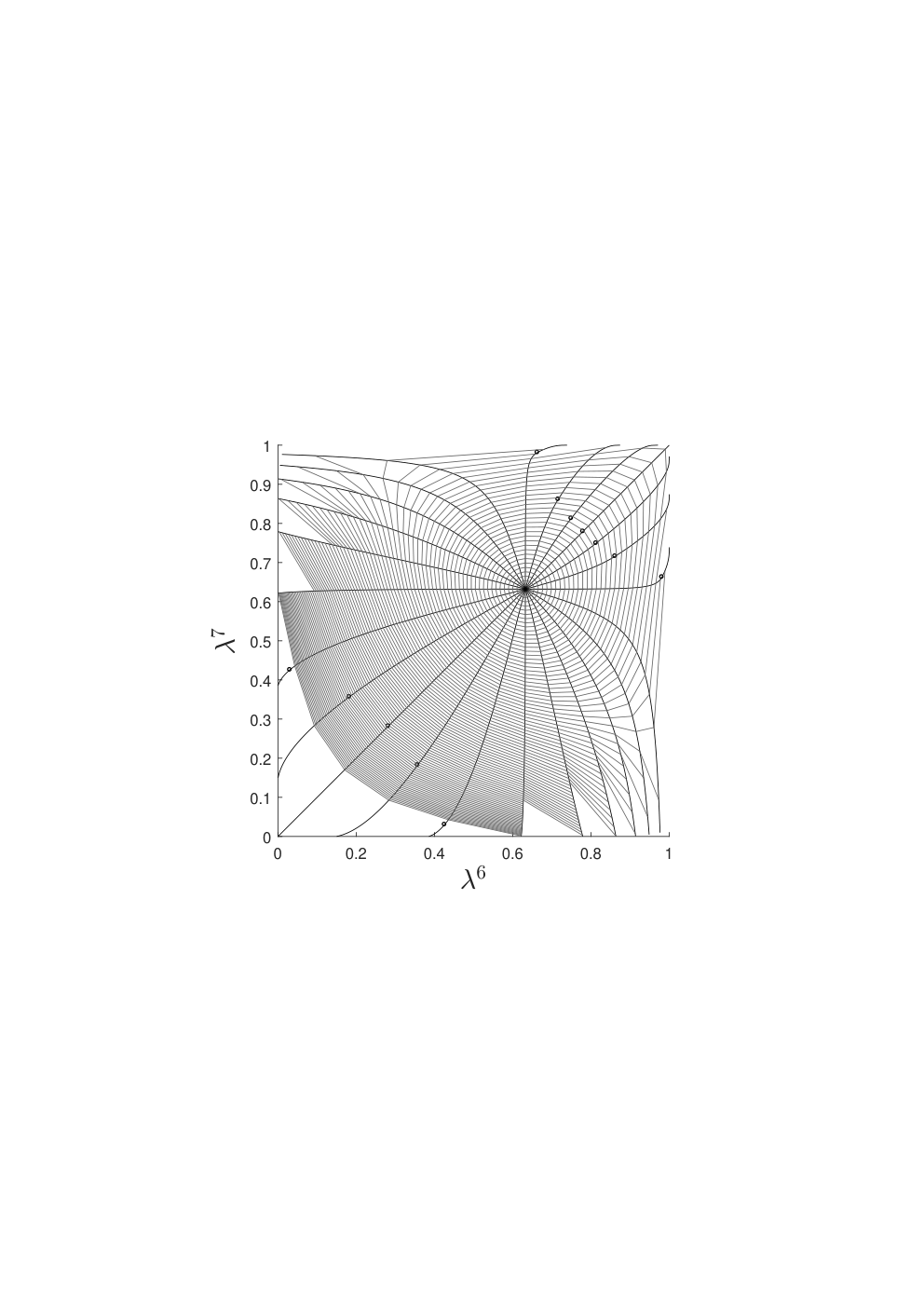
Figure 4 shows typical results. The figure shows the orthant representing the two internal edge lengths, with geodesics ‘fired’ from some fixed starting point $\boldsymbol{\ell}_{0}$ in $24$ different directions. Also marked on the plots are contours of distance from the starting point. Each panel shows results for a different initial tree $\boldsymbol{\ell}_{0}$. It is evident that the geodesics are not the same as BHV geodesics, which are straight lines radiating from the initial point with equally spaced circular contours of distance. Figure 4 shows curved geodesics with irregularly spaced contours of distance. Contours appear to stack up towards the origin and codimension-1 BHV boundaries, but are more spaced out as geodesics move out towards the boundaries at infinity. This is more obvious when initial internal edges are long (top row of Figure 4). On the other hand, the geodesics are more similar to the BHV geodesics when internal edges are short and pendant edges are long, as in the bottom two rows of the right hand column. In all cases, in contrast to BHV tree space, geodesics seem to be slightly attracted toward the star trees. The pendant edges do not behave as they do in BHV tree space: they can change value even when their initial velocity is zero.

Figure 5 provides more detail for certain geodesics in Figure 4. The graphs in the figure show each edge weight $\lambda^{i}$ versus time, and the time is proportional to distance travelled. The $\boldsymbol{\lambda}$-parametrization was used for these plots since it shows the results most clearly. Panel (a) shows that, when contours become more and more widely spaced, the boundary at infinity ($\lambda^{6}=\lambda^{7}=1$) can be reached in finite time, rather than asymptotically. This shows that points corresponding to trees with infinitely long edges are a finite distance away from the starting point, as established by Theorem 3.2. In the $\boldsymbol{\ell}$-parametrization, the internal edge lengths rapidly blow up to infinity after time $t=0.8$. It follows that the shortest path between two trees with finite edge lengths might involve trees with infinitely long edges. On the other hand, for some panels in Figure 4, the contours become increasingly close as BHV boundaries are approached, but as panel (b) in Figure 5 shows, points on BHV boundaries are in fact finitely close to orthant interiors, since the boundary is reached in finite time.

Figure 6 replots the top left and middle left panels from Figure 4 using the $\boldsymbol{\lambda}$-parametrization, so that the boundary at infinity corresponds to edges of the unit square with weight $1$. These plots suggest that trees in which one of the two internal edges is finitely long are ‘repellant’ since the geodesics fired in the North and East compass directions end up passing through the disconnected forest with $\lambda^{6}=\lambda^{7}=1$. Indeed, the points on the boundary with $\lambda^{6}=\lambda^{7}=1$ appear to be ‘attractive’, with geodesics pulled round to pass through these points and arriving in finite time.

While these results show how the information geometry on $\mathcal{W}_{N}$ differs substantially from the BHV geometry, the method for constructing geodesics by integrating the geodesic differential equation suffers from several disadvantages. First, it requires summation over the elements of $\{0,1\}^{N}$ which makes it infeasible for large $N$ (exponential computation time in $N$). Secondly, only local geodesics are computed by solving the initial value problem (geodesic “shooting” or “firing”) for the differential equation valid only in maximal orthants. Thirdly, for practical applications, an algorithm which takes two points in wald space and joins them by a globally shortest path is more useful, and so it is desirable to solve the boundary value problem for geodesic construction. The next section attempts to deal with some of these shortcomings.

Our aim is to construct a Gaussian process which is a continuous-valued analogue of the symmetric two-state process by matching the moments specified in Lemma 2.1. Consider the Ornstein-Uhlenbeck process $Z(t)$ on $T$ which satisfies

where $\ell_{t_{1}t_{2}}$ is the path length distance between $t_{1}$ and $t_{2}$ on $T$. The stationary distribution is the standard normal distribution $N(0,1)$, and we assume the process is stationary over $T$. The Markov process satisfies the detailed balance equation, and so is reversible in its stationary state. As a result, realizations of the process can be simulated by fixing an arbitrary root $t_{0}\in T$ for the tree, simulating $Z(t_{0})$ from $N(0,1)$ and then using Equation (8) to simulate a realization $Z(t)$ for any other $t\in T$. Reversibility of the process ensures the distribution obtained is invariant of the choice of root. A short calculation shows that the covariance matrix of the random variables $Z_{1},\ldots,Z_{N}$ at the leaves of $T$ is given by $\mathrm{Cov}\left(Z_{u},Z_{v}\right)=\exp(-\ell_{uv})$. Since $\ell_{uu}=0$ for all $u=1,\ldots,N$, this gives $\mathrm{Var}\left(Z_{u}\right)=1$. Similarly, the conditional distribution of $Z(t_{2})$ given $Z(t_{1})=z$ has variance $1-\exp(-2\ell_{t_{1}t_{2}})$. These moments match those in Lemma 2.1 up to the constant factor of $1/4$, and we will show later that this factor makes no difference to the geometry obtained. The process $Z(t)$ can be thought of in two ways. First, it approximates the binomial random variables obtained when many independent binary characters evolve under the symmetric two-state process. Secondly, it could be regarded as an evolutionary model of a continuous trait for which the observations are standardized to have zero mean and unit variance in each population. Mean-reverting Gaussian processes like this are sometimes used to model continuous traits for which there is some constant optimal value for survival (Hansen and Martins 1996). The definition of $Z(t)$ extends from trees to forests by taking the process to be independent on each connected component.

Given a forest $F\in W_{N}$, the distribution of the random variables $Z_{1},\ldots,Z_{N}$ at the leaves is multivariate normal with zero mean and covariance matrix $S_{F}$ where

The path distance $\ell_{uv}$ is the sum of the lengths $\ell^{e}$ on edges $e$ between $u$ and $v$, and is taken to be infinite when $u$ and $v$ are in different components of $F$. This defines a map $F\mapsto\phi_{F}$ from forests to multivariate normal distributions where $\phi_{F}$ is the probability density function of $N(\boldsymbol{0},S_{F})$. A similar result to Lemma 2.3 holds: whenever $F_{1}\sim F_{2}$, the distributions $\phi_{F_{1}}$ and $\phi_{F_{2}}$ are the same, so the map is well-defined on $\mathcal{W}_{N}$.

The information geometry of multivariate normal distributions with zero mean has been studied previously (Lenglet et al. 2006) and is analytically tractable. The theory described in Section 3 needs adapting to account for the change from discrete to continuous characters. The Fisher information metric of $\mathcal{W}_{N}$ in Equation (4) becomes an integral over $\mathbb{R}^{N}$ rather than a sum, and the mass function $p_{\boldsymbol{\ell}}$ is replaced with the density function $\phi_{\boldsymbol{\ell}}$ of the Gaussian corresponding to a fully resolved tree with edge lengths $\boldsymbol{\ell}$:

The geodesic equation (5) remains the same. Although $p_{T}(s)$ and its derivatives could be evaluated exactly for the two-state symmetric model, evaluation of the metric and Christoffel symbols required a sum over all characters. For the continuous model, the corresponding integrals have closed form, as we describe below.

Gaussian distributions with zero mean are parametrized by their covariance matrices, namely by the space of $N\times N$ symmetric positive definite matrices, which we will denote $\mathcal{S}^{+}_{N}$. The set of covariance matrices associated with forests forms a subset within $\mathcal{S}^{+}_{N}$, as determined by the following theorem.

The proof is given in the Appendix.

For Gaussians with zero mean, it can be shown that the Fisher information metric at a point with covariance matrix $S$ is

where $X,Y$ are matrices in the tangent space at $S$, i.e. symmetric matrices (Lenglet et al. 2006). This expression is obtained by evaluating the integral in Equation (10). Working in some fixed maximal orthant parametrized by edge lengths $\boldsymbol{\ell}$, let $S_{\boldsymbol{\ell}}$ be the corresponding covariance matrix defined in Equation (9). For each edge $e\in F$ define the split matrix $\sigma^{e}$ by

for $u,v=1,\ldots,N$. Then the path length between $u$ and $v$ is $\ell_{uv}=\sum_{e}\ell^{e}\sigma^{e}_{uv}$ where the sum is over all edges in $F$. Equation (9) becomes

An entry above is zero if $u$ and $v$ are in different connected components, or equivalently, if they are separated by an infinitely long edge.

By differentiating Equation (12), it can be seen that the tangent space at $S_{\boldsymbol{\ell}}$ is spanned by matrices of the form $\sigma^{e}\circ S_{\boldsymbol{\ell}}$ for each edge $e$, where $\circ$ denotes the Hadamard matrix product. The Fisher information metric (10) for $\mathcal{W}_{N}$ for a fully resolved tree becomes

where $i,j=1,\ldots,2N-3$ index edges. Algebraic expressions for the first and second derivatives of the Fisher information metric can similarly be obtained, and hence for the Christoffel symbols. Note that scaling $S_{\boldsymbol{\ell}}$ by some positive constant has no effect on the metric, and so the factor of $1/4$ difference between the covariance matrices obtained from the discrete process $X(t)$ and continuous process $Z(t)$ has no effect on the geometry.

The inner product and its derivatives can be computed in polynomial time and the paths obtained by integrating the geodesic ODE for the continuous Markov model within orthant interiors in $\mathcal{W}_{N}$ resemble those for the two-state model very closely. Namely, results for the same initial conditions as Figure 4 were obtained but omitted, since the plots were almost indistinguishable from those for the two-state model. However, the inner products defined using the two different models are not identical: both inner products can be written down explicitly in the case $N=2$, using the transition probabilities for the discrete model and Equation (13) for the continuous model. The two inner products differ when the length of the single edge in the tree is small, but converge as the edge length tends to infinity.

Using Equation (13) and its derivatives, we derived algebraic expressions for the Riemannian curvature tensor and the sectional curvatures at any point in $\mathcal{W}_{N}$. We implemented these expressions in R, and hence evaluated these quantities for certain trees in $\mathcal{W}_{5}$. We found that at randomly selected points in $\mathcal{W}_{5}$, and hence in all spaces with $N\geq 5$, the sectional curvatures had mixed signs. As a result, there is no global sign condition on curvature like that for BHV tree space, which is globally non-positively curved.

To approximate geodesics in the extrinsic covariance metric $d_{\mathrm{cov}}$ of $\mathcal{W}_{N}$, we construct a projection from $\mathcal{S}^{+}_{N}$ onto $\mathcal{W}_{N}$, that is, given $S_{0}\in\mathcal{S}^{+}_{N}$, we aim to find an element $[F]\in\mathcal{W}_{N}$ which minimizes $d_{\mathrm{cov}}(S_{0},S_{F})$. Suppose that $F$ is a fully resolved tree with edge lengths $\boldsymbol{\ell}$. The expression for $d_{\mathrm{cov}}(S_{0},S_{F})^{2}$ can be differentiated with respect to edge lengths of $F$ and gives

where $\partial_{i}=\partial/\partial_{\ell^{i}}$ (e.g. Moakher 2005). Moreover, $\partial_{i}S_{F}=S_{F}\circ\,\sigma^{i}$ where $\circ$ denotes the Hadamard or element-wise matrix product and $\sigma^{i}$ is the split matrix associated with edge $i$, as defined in Equation (11).

This analytic expression for the derivative can be used to implement a gradient descent algorithm. Within each maximal orthant $\mathcal{O}_{\tau}$ the edge lengths were updated according to the rule

where $\boldsymbol{\ell}_{k}$ denotes the edge lengths at iteration $k$ and $S_{\boldsymbol{\ell}_{k}}$ the corresponding covariance matrix. The step size $\alpha_{k}$ was determined using the Barzillai-Borwein method. Two versions of the algorithm were used. In the first, the algorithm was halted whenever an internal edge was assigned a negative length. As a result, the algorithm was constrained to lie within the orthant $\mathcal{O}_{\tau}$ containing the initial tree. This algorithm was used for $N=5$ by running the algorithm $15$ times, each time with an initial tree in one of the 15 maximal orthants of $\mathcal{U}_{5}$, and the overall tree closest to $S_{0}$ found. The second version of the algorithm was able to cross codimension-$1$ BHV boundaries as follows. If an edge length was assigned a negative value, then trees in the two corresponding neighbouring orthants to $\tau$ were considered, taking the absolute value of elements in $\boldsymbol{\ell}_{k+1}$ as edge lengths. The tree at step $k+1$ was taken to be whichever of these two trees was closest to $S_{0}$.

In general, the closest point in $\mathcal{W}_{N}$ to a covariance matrix $S_{0}\in\mathcal{S}^{+}_{N}$ is not necessarily unique as illustrated in Figure 8. Moreover, the gradient descent algorithm can converge to local minima, and so the result obtained is sensitive to the tree used to initialize the algorithm.

Since construction of geodesics in $\mathcal{S}^{+}_{N}$ between any two given points and projection from $\mathcal{S}^{+}_{N}$ into $\mathcal{W}_{N}$ can both be performed efficiently, we aim to combine these algorithms to give an efficient means of constructing geodesics within $\mathcal{W}_{N}$ between any two given end points. A naive approach, given $[F_{1}],[F_{2}]\in\mathcal{W}_{N}$, is to simply project the extrinsic geodesic between $S_{F_{1}}$ and $S_{F_{2}}$ from $\mathcal{S}^{+}_{N}$ into $\mathcal{W}_{N}$. This approach works for the example of the unit sphere $S^{2}$ embedded within $\mathbb{R}^{3}$: the projection of the chord between two points in the sphere is a great circle between those two points. However, this approach fails for $\mathcal{W}_{N}\subseteq\mathcal{S}^{+}_{N}$ since the projected paths are often discontinuous and jump between different orthants, as illustrated in Figure 8.

The following recursive algorithm for constructing an approximate geo-desic in $\mathcal{W}_{N}$ is therefore proposed, which is intended to overcome this issue. Let $t_{i}=i/k$ for $i=0,\ldots,k$ and suppose $[F_{1}],[F_{2}]\in\mathcal{W}_{N}$. The algorithm outputs a sequence $[G_{0}],\ldots,[G_{k}]\in\mathcal{W}_{N}$ where $[G_{0}]=[F_{1}]$ and $[G_{k}]=[F_{2}]$. For each iteration $i=1,\ldots,k-1$ of the algorithm, the following steps are performed.

References

- Adams and Castoe (2019) Adams, R. H. and Castoe, T. A. (2019). Probabilistic species tree distances: implementing the multispecies coalescent to compare species trees within the same model-based framework used to estimate them. Syst. Bio.
- Allen and Steel (2001) Allen, B. L. and Steel, M. (2001). Subtree transfer operations and their induced metrics on evolutionary trees. Ann. Comb., 5(1):1–15.
- Allman et al. (2008) Allman, E. S., Ané, C., and Rhodes, J. A. (2008). Identifiability of a Markovian model of molecular evolution with gamma-distributed rates. Adv. Appl. Probab., 40(1):229–249.
- Ballmann et al. (1985) Ballmann, W., Gromov, M., and Schroeder, V. (1985). Manifolds of nonpositive curvature, volume 61 of Progress in mathematics. Birkhäuser.
- Bačák (2014) Bačák, M. (2014). Computing medians and means in Hadamard spaces. SIAM J. Optim., 24(3):1542–1566.
- Billera et al. (2001) Billera, L., Holmes, S., and Vogtman, K. (2001). Geometry of the space of phylogenetic trees. Adv. Appl. Math., 27:733–767.
- Bridson and Haefliger (2011) Bridson, M. R. and Haefliger, A. (2011). Metric Spaces of Non-Positive Curvature. Springer, Berlin.
- Bryant et al. (2005) Bryant, D., Galtier, N., and Poursat, M.-A. (2005). Likelihood calculation in molecular phylogenetics. In Gascuel, O., editor, Mathematics of Evolution and Phylogeny, pages 33–62. Oxford University Press.
- Dryden et al. (2009) Dryden, I. L., Koloydenko, A., Zhou, D., et al. (2009). Non-Euclidean statistics for covariance matrices, with applications to diffusion tensor imaging. Ann. Appl. Stat., 3(3):1102–1123.
- Engström et al. (2013) Engström, A., Hersh, P., and Sturmfels, B. (2013). Toric cubes. Rendiconti del Circolo Matematico di Palermo, 62(1):67–78.
- Feragen et al. (2013) Feragen, A., Owen, M., Petersen, J., Wille, M., Thomsen, L., Dirksen, A., and de Bruijne M. (2013). Tree-space statistics and approximations for large-scale analysis of anatomical trees. In 23rd biennial International Conference on Information Processing in Medical Imaging (IPMI).
- Garba (2019) Garba, M. K. (2019). Information geometry for phylogenetic trees. PhD thesis, School of Mathematics, Statistics and Physics, Newcastle University.
- Garba et al. (2018) Garba, M. K., Nye, T. M. W., and Boys, R. J. (2018). Probabilistic distances between trees. Syst. Bio., 67(2):320–327.
- Gill et al. (2008) Gill, J., Linusson, S., Moulton, V., and Steel, M. (2008). A regular decomposition of the edge-product space of phylogenetic trees. Adv. Appl. Math., 41(2):158–176.
- Hansen and Martins (1996) Hansen, T. F. and Martins, E. P. (1996). Translating between microevolutionary process and macroevolutionary patterns: the correlation structure of interspecific data. Evolution, 50(4):1404–1417.
- Huelsenbeck and Ronquist (2001) Huelsenbeck, J. P. and Ronquist, F. (2001). MrBayes: Bayesian inference of phylogenetic trees. Bioinformatics, 17(8):754–755.
- Kim (2000) Kim, J. (2000). Slicing hyperdimensional oranges: The geometry of phylogenetic estimation. Mol. Phylogenet. Evol., 17(1):58–75.
- Lee (1997) Lee, J. M. (1997). Riemannian manifolds: an introduction to curvature, volume 176. Springer.
- Lenglet et al. (2006) Lenglet, C., Rousson, M., Deriche, R., and Faugeras, O. (2006). Statistics on the manifold of multivariate normal distributions: Theory and application to diffusion tensor MRI processing. J. Math. Imaging Vis., 25(3):423–444.
- Lin et al. (2018) Lin, B., Monod, A., and Yoshida, R. (2018). Tropical foundations for probability and statistics on phylogenetic tree space. arXiv preprint arXiv:1805.12400.
- Lin and Yoshida (2018) Lin, B. and Yoshida, R. (2018). Tropical Fermat–Weber points. SIAM J. Discrete Math., 32(2):1229–1245.
- Miller et al. (2015) Miller, E., Owen, M., and Provan, J. S. (2015). Polyhedral computational geometry for averaging metric phylogenetic trees. Adv. Appl. Math., 68:51–91.
- Moakher (2005) Moakher, M. (2005). A Differential Geometric Approach to the Geometric Mean of Symmetric Positive-Definite Matrices. SIAM J. Matrix Analysis Applications, 26:735–747.
- Moulton and Steel (2004) Moulton, V. and Steel, M. (2004). Peeling phylogenetic oranges. Adv. Appl. Math., 33(4):710–727.
- Nye (2014) Nye, T. (2014). An algorithm for constructing principal geodesics in phylogenetic treespace. IEEE ACM T. Comput. Bi., 11(2):304–315.
- Nye (2011) Nye, T. M. W. (2011). Principal components analysis in the space of phylogenetic trees. Ann. Statist., 39(5):2716–2739.
- Nye et al. (2017) Nye, T. M. W., Tang, X., Weyenberg, G., and Yoshida, R. (2017). Principal component analysis and the locus of the Fréchet mean in the space of phylogenetic trees. Biometrika, 104(4):901–922.
- Owen and Provan (2011) Owen, M. and Provan, J. S. (2011). A fast algorithm for computing geodesic distances in tree space. IEEE ACM T. Comput. Bi., 8(1):2–13.
- Rogers (1997) Rogers, J. S. (1997). On the consistency of maximum likelihood estimation of phylogenetic trees from nucleotide sequences. Systematic biology, 46(2):354–357.
- Sason and Verdu (2016) Sason, I. and Verdu, S. (2016). -divergence inequalities. IEEE Transactions on Information Theory, 62(11):5973–6006.
- Schmidt et al. (2006) Schmidt, F. R., Clausen, M., and Cremers, D. (2006). Shape matching by variational computation of geodesics on a manifold. In Joint Pattern Recognition Symposium, pages 142–151. Springer.
- Semple and Steel (2003) Semple, C. and Steel, M. (2003). Phylogenetics, Oxford Lecture Series in Mathematics and its Applications, 24. Oxford University Press.
- Skovgaard (1984) Skovgaard, L. T. (1984). A Riemannian geometry of the multivariate normal model. Scand. J. Stat., 11(4):211–223.
- Speyer and Sturmfels (2004) Speyer, D. and Sturmfels, B. (2004). The tropical Grassmannian. Adv. Geom., 4(3):389–411.
- Steel and Penny (1993) Steel, M. A. and Penny, D. (1993). Distributions of tree comparison metrics – some new results. Syst. Biol., 42(2):126–141.
- Willis (2019) Willis, A. (2019). Confidence sets for phylogenetic trees. J. Am. Stat. Assoc., 114(525):235–244.
- Yang (2006) Yang, Z. (2006). Computational molecular evolution. Oxford University Press.
- Yoshida et al. (2019) Yoshida, R., Zhang, L., and Zhang, X. (2019). Tropical principal component analysis and its application to phylogenetics. B. Math. Biol., 81(2):568–597.
- Zwiernik and Smith (2012) Zwiernik, P. and Smith, J. Q. (2012). Tree cumulants and the geometry of binary tree models. Bernoulli, 18(1):290–321.