A Decentralized Policy with Logarithmic Regret for a Class of Multi-Agent Multi-Armed Bandit Problems with Option Unavailability Constraints and Stochastic Communication Protocols

This paper considers a multi-armed bandit (MAB) problem in which multiple mobile agents receive rewards by sampling from a collection of spatially distributed stochastic processes, with the goal of maximizing the total cumulative reward of all agents. Each agent is allowed to communicate only with a limited number of neighboring agents. The problem formulation is motivated by applications in which a team of autonomous mobile robots cooperates to accomplish a spatially distributed task in an uncertain environment. Examples might include prospecting for and collecting mineral resources, or finding and marking unexploded ordnance. Movement constraints on the agents are described by a connected spatial graph with vertices representing the sampling options, and with edges representing directly connected options and the distances between those options. Communication connectivity between agents is described by a second non-stationary stochastic graph, which describes the subset of agents from which data may be received at a particular time. The limited communication makes it infeasible to direct all agents from a central location with perfect knowledge of the entire sampling history. Instead, each agent implements a decentralized policy, based only on local information.

It is known that optimal policies for MAB problems must intersperse exploitation – that is, repeated sampling of the option with the highest expected reward – with exploration – that is, sampling of options with lower expected rewards in order to reduce uncertainty about their distributions [1, 2, 3, 4]. The loss of reward due to exploration is called regret. In the standard MAB problem minimizing regret is equivalent to maximizing reward. For the case of a single agent on a fully connected spatial graph, it is known that the optimal expected regret is asymptotically bounded below by a function that grows as the logarithm of time [4]. A class of policies called upper confidence bound (UCB) algorithms asymptotically achieve logarithmic regret for the classical MAB problem [5, 6, 7, 8, 9, 10].

The class of problems we consider in this paper fall under the broad category of decentralized multi agent multi armed bandit problems (D-MAMAB) [11, 12, 13, 14, 15]. A running consensus, with agents observing the estimates of other agents through communication, is employed in [12, 14, 15]. Fixed graphs as well as stationary stochastic communication graphs are considered in these studies. A brief review of the existing D-MAMAB schemes that use a running consensus of the estimates is provided in [15]. They also propose a novel running consensus based algorithm that results in a lower regret than the other existing consensus based algorithms. In contrast the work by [13] considers a D-MAMAB scheme where the agents use a fixed communication graph to communicate only the instantaneous rewards obtained by the agents. This ideas is extended to the case of an independently and identically distributed Erdős-Rényi (ER) graph based stochastic communication policy in [14, 16].

In this paper, we propose a UCB-based movement and option selection policy and a non-stationary stochastic communication protocol which, to our knowledge, is the first decentralized policy guaranteeing asymptotically logarithmic regret for non-fully connected spatial graphs with communication constraints. When the spatial graph is fully connected and the communication graph is stationary, our decentralized algorithm matches or exceeds the best reported prior results from the literature. The communication protocol requires transmission only of the agent’s most recent measurement. Therefore communication bandwidth requirements are moderate, and no storage of past measurements is required. The paper considers various ways in which performance may be improved, including the dependence on parameters such as the total number of agents, the number of agents communicating at a given time, and the mobility of the agents.

The UCB based based policy that we propose utilizes a reward estimate that depends both on the option rewards obtained by the agent itself as well as those communicated by its neighbors. Redundancies in choice, due to two or more neighbors selecting the same option, are disregarded in the estimation. Each agent maintains an estimate of the rewards obtained by all other agents solely depending on the communicated rewards. Thus these estimates represent, in a certain sense, the belief that each agent has of the estimates that the other agents make. The paper proves that this policy guarantees a logarithmically bounded self regret irrespective of the communication strategy that the agents choose. In the proposed UCB based communication strategy the agents communicate with other agents who they believe to are most likely to be exploring. This in contrast to running consensus schemes, where the agents attempt to synchronize their estimates, the approach used here allows communication to be fully utilized for exploration. A preliminary version of these results on a fully connected spatial graph was presented in [17].

In section II we present the notations and a precise definition of the class of D-MAMAB problems that is considered in this paper. Section III proposes the novel UCB based policy. This section also proves that the policy guarantees logarithmic regret. It also shows that the regret reduces with increasing connectivity. The effectiveness of the proposed scheme is demonstrated through simulations in section IV.

This section defines the Decentralised Multi Agent Multi Armed Bandit (D-MAMAB) problem that is considered in this paper. At any given time an agent will only have access to a limited set of options. The options will be assumed to be distributed along the vertices of a fixed connected graph and the agents will be allowed to move from one vertex to another along the edges of the graph. At a given time step an agent can only move along one edge of the graph. An agent is only allowed to pick the option that is located at the vertex it occupies. The agents may choose which vertex to move to, sample or not the option at the vertex it occupies, and choose which agents to communicate with. When agents communicate with each other they only share the value of the option it has sampled at that time instance. Such a choice that does not depend on any global information is called a decentralized policy. The MAMAB problem that we will deal with in this paper is that of designing a suitable decentralized policy that maximizes the reward obtained by every agent. This will also ensure that the total network reward is maximized. In what follows we will provide a formal statement of this objective.

Let the total number of agents be denoted by $n_{A}$ and indexed by the set $\{1,2,\cdots,n_{A}\}$. The options and the reward associated with each option are assumed to satisfy the following explicit assumptions:

The random variable $\varphi_{k}^{t}$ corresponds to the option that is chosen by agent $k$ at time $t$. At time $t$ a given agent $k$ is at some vertex $n_{k}^{t}\in\mathcal{V}^{o}$ and it will decide to choose the option at $n_{k}^{t}$ or to refrain from choosing it. In the latter instance we set $\varphi_{k}^{t}=\varnothing$. At the time step $t$ it will also decide on a set of agents $\mathcal{N}_{k}^{t}\subseteq\{1,2,\cdots,n_{A}\}$ to communicate with. The only information that an agent receives from another agent is the option that it has chosen, $\varphi_{k}^{t}$, and the corresponding reward, $X_{\varphi_{k}^{t}}^{t}$. For mathematical completeness we set $X_{\varphi_{k}^{t}}^{t}\equiv 0$ when $\varphi_{k}^{t}=\varnothing$. The resulting communication graph is allowed to be directed. The discrete random variable $\mathcal{N}_{k}^{t}$ will be referred to as the neighbors of agent $k$ at time $t$. By convention we let $k\in\mathcal{N}_{j}^{t}$. Let $\mathcal{N}_{k\alpha}$ be a subset of $\left\{1,2,\cdots,n_{A}\right\}$ that contains $k$ and let $\mathcal{N}_{kP}$ be the space of all such subsets of $\left\{1,2,\cdots,n_{A}\right\}$ (there are a total number of $|\mathcal{N}_{kP}|=2^{(n_{A}-1)}$ such sets). Then the discrete random variable $\mathcal{N}_{k}^{t}$ takes values in the set $\mathcal{N}_{kP}$. Based on the information it has obtained at time $t$, either by sampling the options on its own or through communication, the agent $k$ may decide to move to another vertex $n_{k}^{t+1}\in\mathcal{V}^{o}$ that is in the neighborhood of $n_{k}^{t}$ at time $t+1$. If so desired the agent is also allowed to remain at the vertex it occupies. A neighborhood of an option $i\in\mathcal{V}^{o}$ will be denote by $\mathcal{I}_{i}\subseteq\mathcal{V}^{o}$. The triple $\pi_{j}^{t}\triangleq(n_{j}^{t},\varphi_{j}^{t},\mathcal{N}_{j}^{t})$ is the outcome of a suitable policy that will only depend on the information available to agent $j$ at time $t-1$. Let $\mathcal{F}^{t}_{j}$ be the sigma algebra generated by the random variables $\{(\mathcal{N}_{j}^{\nu},n_{j}^{\nu},\{X_{\varphi_{k}^{\nu}}^{\nu}\}_{k\in\mathcal{N}_{j}^{\nu}})\}_{\nu=1}^{t}$ and $\mathcal{F}^{1}_{j}\subset\mathcal{F}^{2}_{j}\subset\cdots\mathcal{F}^{t}_{j}$ be the corresponding filtration. Then the policy $\pi_{j}^{t}$ is a $\mathcal{F}^{t-1}_{j}$ measurable random variable.

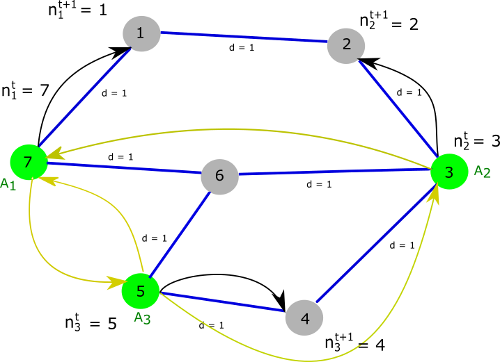We pause for a while to illustrate the problem considered in this paper using a simple example. The example is for a seven option three agent MAMAB problem. It is represented using figure 1. Let $\mathcal{G}^{o}=(\mathcal{V}^{o},\mathcal{E}^{o})$ be the fixed un-directed graph shown in this figure. The vertices $\mathcal{V}^{o}=\{1,2,\cdots,7\}$ are shown by circles while the edges $\mathcal{E}^{o}$ are indicated by the blue lines in figure 1. The seven options of the bandit are taken to be distributed along the vertices of the graph $\mathcal{G}^{o}=(\mathcal{V}^{o},\mathcal{E}^{o})$ while the edges indicate the paths that an agent can follow. The distance between any two adjacent nodes of the graph is taken to be $d=1$. The agents are labelled $\{A_{1},A_{2},A_{3}\}$ and the nodes they occupy at time $t$ are highlighted by the color green. Thus we have that $n_{1}^{t}=7,n_{2}^{t}=3,n_{3}^{t}=5$. Based on the information an agent has, that is made available solely through exploration or communication with neighbors up to time $t$, it will decide at time $t+1$ to move to a neighbor of the option that it occupied at $t$. For instance at the time step $t+1$ agent $A_{2}$ can only move to the options in the neighborhood of the option $3$ that is given by the set $\mathcal{I}_{3}=\{2,4,6\}$. The black arrows in this example indicate the node that each agent has decided to move. Accordingly we see that $A_{2}$ has decided to move to option 2 at time $t+1$ (ie. $n_{2}^{t+1}=2$). The agents then decide whether or not to sample the option that is located at the node it had moved to and which agents to communicate with based on the information it had at $t$. If agent $A_{2}$ decides to choose option 2 at time $t+1$ we set $\varphi_{2}^{t+1}=2$ or if otherwise we set $\varphi_{2}^{t+1}=\varnothing$. The yellow arrowed lines denote the directed edges of the communication graph at time $t$. Thus, for instance, according to our notation we have $\mathcal{N}_{1}^{t}=\{1,3\}$, $\mathcal{N}_{2}^{t}=\{2,1\}$ and $\mathcal{N}_{3}^{t}=\{3,1,2\}$.

The indicator random variable corresponding to an event $\mathcal{M}$ will be denoted by $\mathbb{I}_{\mathcal{M}}$. Then $\mathbb{I}_{\{\varphi_{k}^{t}=i\}}$ represent if the option $i$ was picked by agent $k$ at time $t$ and hence is a $\mathcal{F}^{t-1}_{k}$ measurable Bernoulli random variable. The cumulative reward obtained by agent $j$ by sampling option $i$ in the time horizon $[1,T]$ is defined by $S^{s}_{ij}(T)\triangleq\sum_{t=1}^{T}X_{i}^{t}\mathbb{I}_{\{\varphi_{j}^{t}=i\}}$.Then the total reward obtained by agent $j$ is $S^{s}_{j}(T)\triangleq\sum_{i\in\mathcal{V}^{o}}S^{s}_{ij}(T)$ and the total reward of the network is $S^{s}(T)\triangleq\sum_{j=1}^{n_{A}}\sum_{i\in\mathcal{V}^{o}}S^{s}_{ij}(T)$.

In the standard single agent MAB problem maximizing the reward is equivalent to minimizing the regret. Each time an agent adds the reward of a suboptimal option to its collected reward it also accumulates a regret that is equal to the difference between the optimal reward and the added suboptimal reward. Therefore the total cumulative self regret of the $j^{\mathrm{th}}$ agent, due to the sub optimal option $i$ being chosen by $j$ within the time horizon $T$ is defined to be

Here the $\mathcal{F}^{t-1}$ measurable random variable

denotes the total number of times that agent $j$ has chosen $i$ in the time horizon $[1,t]$. Then the above expression for the regret takes the form $R^{s}_{ij}(T)\leq\bar{\Delta}\mathbb{E}\left(N^{s}_{ij}(T)\right)$. This says that the individual agent self regret per non optimal option is bounded above by the expectation of the number of times that the agent has sampled the suboptimal option in the time horizon $[1,T]$. The total regret accrued by agent $j$ is simply the summation of $R^{s}_{j}(T)\triangleq\sum_{i\neq i_{*}}R^{s}_{ij}(T)$ over all suboptimal options and the total network regret is obtained by summing this over all agents $R^{s}(T)\triangleq\sum_{j=1}^{n_{A}}\sum_{i\neq i_{*}}R^{s}_{ij}(T)$. Hence, in order to simplify the notation, it suffices to only consider the regret per suboptimal option per agent where the total network values can be obtained by summing over all suboptimal options and agents.

The $\mathcal{F}^{t-1}_{j}$ measurable Bernoulli random variable

contains the information whether $j$ has received information of $i$ being picked either by itself or by one of its neighbors at time $t$. Typically the policy $\pi_{j}^{t}=(n_{j}^{t},\varphi_{j}^{t},\mathcal{N}_{j}^{t})$ depends on the estimates that one makes of $\mathbb{E}\left(X_{i}^{t}\right)$. The best possible approach to estimating the conditional expectation of $X_{i}^{t}$ is to use the full information one has access to. One such approach is to use the sample mean estimate, $\widehat{X}_{i}^{t}$, that is defined by

We set ${X}_{ik}^{0}=\bar{x}_{ik}$ and $\widehat{\mu}_{ik}^{0}=\bar{x}_{ik}$ and $N_{ik}^{0}=1$ for all $i,k$ where $\bar{x}_{ik}$ are generated from some distribution representing a prior belief of the options. The random variable $\widehat{X}_{ik}^{t}$ is the conditional sample mean of $X_{i}^{t}$ that is estimated by the agent $k$. The random variable $N_{ij}(t)$ is the $\mathcal{F}_{j}^{t-1}$ measurable random variable that denotes the total number of times that $j$ has received information of $i$ being picked either by itself or by one of its neighbors at time $t$. The random variable $N^{c}_{ij}(t)\triangleq\sum_{\nu=1}^{t}\mathbb{I}_{\{\varphi_{j}^{\nu}\neq i\>\&\>\epsilon_{ij}^{\nu}=1\}}$ represents the number of times that agent $j$ has received information of option $i$ purely through means of communication.

A Hoeffding type tail bound is provided in Theorem 4 of [8] for the random summand of pre-visible random variables. Setting $X_{t}=X_{r}^{t}$, $Y(t)=Y_{rk}(t)\triangleq\sum_{t=1}^{T}\left(X_{r}^{t}-\mathbb{E}\left(X_{r}^{t}\right)\right)\epsilon_{rk}(t)$, $\epsilon_{t}=\epsilon_{rk}(t)$, and $N(t)=\sum_{\tau=1}^{t}\epsilon_{rk}^{\tau}$ in this result it follows that the sample mean estimator defined by (3) – (4) satisfies the tail bound

where $\eta>0$ is a constant, $\Phi(t)$ is some positive function of $t$ and $\widehat{\mu}_{rk}^{t}$ is defined by

Expression (5) represents the belief that the agent $k$ has of the estimate of the reward of option $r$. The number of times that agent $k$ has become aware of $r$ being chosen depends on the policy $\pi_{k}^{t}=(n_{k}^{t},\varphi_{k}^{t},\mathcal{N}_{k}^{t})$. The right hand side says that if the confidence on the belief of the estimate is to increase as $(1-2\vartheta/t^{2})$, where $\vartheta=1/\sqrt{1+\eta}$, then the function $\Phi(t)$ must satisfy $({\sigma}^{2}\sqrt{1+\eta}/\delta_{r}^{2})\log{\left(t\sqrt{\log{(t)}}\right)}\leq\Phi(t)$. On the other hand since

if and only if $N_{rk}(t)\geq\Phi(t)$, by choosing $\Phi(t)=({\sigma}^{2}\sqrt{1+\eta}/\delta_{r}^{2})\log{\left(t\sqrt{\log{(t)}}\right)}$ the following lemma follows.

This in essence implies that if an agent receives information from an option at least logarithmically often then it will be $(1-2\vartheta/t^{2})$ confident that the estimate satisfies $\left|\widehat{X}_{rk}^{t}-\widehat{\mu}_{rk}^{t}\right|\leq\delta_{r}$. Thus since $N_{rk}(t)=N_{rk}^{s}(t)+N_{rk}^{c}(t)$ an agent can increase the confidence that it has of $\widehat{X}_{rk}^{t}$ by means of effective communication.

In this section we propose a decentralized policy for the motion of the agents, $n_{j}^{t}$, the selection of options, $\varphi_{j}^{t}$, and the choice of neighbors to communicate with, $\mathcal{N}_{j}^{t}$, solely based on the information the agent has obtained up to the previous time step. That is, we will develop a $\mathcal{F}_{j}^{t-1}$ measurable policy $\pi_{j}^{t}=(n_{j}^{t},\varphi_{j}^{t},\mathcal{N}_{j}^{t})$ for solving the D-MAMAB problem. The policy will be based on a set of UCB based cost functions that each agent maintains. Namely at each time instance $t$ the agents will (a) chose $n_{j}^{t}$, $\varphi_{j}^{t}$, and $\mathcal{N}_{j}^{t}$ based on the cost function values at $t-1$, and (b) update the cost function values. We will first consider step of choosing $n_{j}^{t}$ and $\varphi_{j}^{t}$ that we will refer to as the UCB based motion allocation and option selection policy and $\mathcal{N}_{j}^{t}$ the UCB based communication policy.

In this section we consider a set of 100 options located at the nodes of a $10\times 10$ two dimensional spatial lattice. The reward associated with each option is assumed to satisfy a Gaussian normal process with variance equal to 2. The intensity of the cell color depicts the size of the mean of the option where the brightest yellow corresponds to the option with the largest mean and the darkest blue corresponds to the option with the smallest mean. The option with the largest mean is the one that occupies the bottom right most corner cell that is highlighted in bright yellow in figure 2 (a). The figure 2 (b) shows the distribution of the numerical values of the means of each of the 100 options.

At the initial time step each agent $k$ initializes its estimates, $\widehat{X}_{ik}^{0}$ by randomly sampling from a probability distribution that represents its prior belief of the option rewards. A time horizon of $T=20,000$ was chosen for each agent and the expectations were estimated by averaging over 20 trials. The total number of agents considered was $n_{A}=20$.

In the case where the communication graph $\mathcal{G}^{t}$ is an iid ER graph process, at each time $t$ the communication graph is an element of, $\mathbb{G}(n_{A},p)$, the space of all possible ER graphs of $n_{A}$ nodes and edge probability $p$. In this case the probability of $j$ having the set of neighbors $\mathcal{N}_{j}^{t}=\mathcal{N}_{j\alpha}$ is given by $\mathcal{P}\left(\mathcal{N}_{j}^{t}=\mathcal{N}_{j\alpha}\right)=p^{|\mathcal{N}_{j\alpha}|-1}(1-p)^{n_{A}-|\mathcal{N}_{j\alpha}|}$. Note that the expectation of the connectivity of the ER graph is given by $\langle|\mathcal{N}_{j\alpha}|\rangle-1=(n_{A}-1)p$. In the case of the UCB based communication policy we restrict the connectivities to a certain fixed value $\gamma$.

Figures 3 shows the estimates of the cumulative self regret, $R^{s}_{ij}(T)$, for several connectivities of the graph for the (a) the iid ER graph communication policy and (b) the UCB based communication policy (12). Figure 3demosntrates how the self regret decreases as communication is increased. A comparison of the two simulations also clearly indicates that the dependent UCB based communication strategy significantly outperforms the independent ER graph based communication. This is further highlighted in figure 4. Finally figure 5 show how the communication effect increases with the expected connectivity and figure shows the effectiveness of the UCB based communication in comparison with the ER graph based random communication.

The paper reports a novel approach for solving a class of MAMAB problems with motion and and communication constraints. The options are taken to be distributed along the nodes of a fixed graph. The agents are free to move from one node to another along the edges of the graph. They can only move one edge at a time and can only pick the option that is located at the node that it occupies. When the graph is fully connected the problem reduces to a decentralized MAMAB problem with no option availability constraints. This paper propose a novel decentralized policy for the motion of the agents and selection of the options that guarantee the logarithmic bounding of the regret for any communication strategy the agents might choose to employ. We investigate the effect of two communication policies for the agents: one that is independent of the information that the agents have and another that depends on the local information an agent has. The former is modeled after an iid ER graph communication strategy while the latter is based on a novel UCB type communication strategy where agents choose to communicate with others who they expect to be exploring at the given time. Using simulations we demonstrate the effectiveness of communication and the superior performance of the UCB type communication policy over the ER graph based communication policy. The simplicity of the scheme makes the scheme scalable and very communication-ally and computationally cost effective. To the best of our knowledge it is the first time that such results have been presented.

References

- [1] J. C. Gittins, “Bandit processes and dynamic allocation indices,” Journal of the Royal Statistical Society. Series B (Methodological), vol. 41, pp. 148–177, 1979.
- [2] R. S. Sutton and A. G. Barto, Introduction to reinforcement learning. MIT Press Cambridge, MA, USA, 1998.
- [3] H. Robbins, Some Aspects of the Sequential Design of Experiments. Springer New York, 1985.
- [4] T. L. Lai and H. Robbins, “Asymptotically efficient adaptive allocation rules,” Advances in applied mathematics, vol. 6, no. 1, pp. 4–22, 1985.
- [5] R. Agrawal, “Sample mean based index policies with o(log n) regret for the multi-armed bandit problem.” Advances in Applied Probabilityl, vol. 27, pp. 1054–1078, 1995.
- [6] P. Auer, N. Cesa-Bianchi, and P. Fisher, “Finite-time analysis of the multi-armed bandit problem.” Machine Learning, vol. 47, pp. 235–256, 2002.
- [7] E. Kauffman, O. Cappe, and A. Garivier, “On bayesian upper confidence bounds for bandit problem,” in International Conference on Artificial Intelligence and Statistics,, Apr 2012, pp. 592–600.
- [8] A. Garivier and E. Moulines, “On upper-confidence bound policies for switching bandit problems,” in Algorithmic Learning Theory, J. Kivinen, C. Szepesvári, E. Ukkonen, and T. Zeugmann, Eds. Berlin, Heidelberg: Springer Berlin Heidelberg, 2011, pp. 174–188.
- [9] E. Kaufmann, O. Cappé, and A. Garivier, “On the complexity of best-arm identification in multi-armed bandit models,” J. Mach. Learn. Res., vol. 17, no. 1, p. 1?42, Jan. 2016.
- [10] P. Reverdy, V. Srivastava, and N. E. Leonard, “Modeling human decisionmaking in generalized gaussian multi-armed bandits,” in Proceedings of the IEEE, vol. 102, April 2014, pp. 544–571.
- [11] D. Kalathil, N. Nayyar, and R. Jain, “Decentralized learning for multiplayer multiarmed bandits,” IEEE Transactions on Information Theory, vol. 60, no. 4, pp. 2331–2345, April 2014.
- [12] P. Landgren, V. Srivastava, and N. E. Leonard, “On distributed cooperative decision-making in multiarmed bandits,” in Proceedings of the Europeon Control Conference (ECC), June 2016, pp. 243 – 248. [Online]. Available: https://arxiv.org/abs/1512.06888
- [13] R. K. Kolla, K. Jagannathan, and A. Gopalan, “Collaborative learning of stochastic bandits over a social network,” in 2016 54th Annual Allerton Conference on Communication, Control, and Computing (Allerton), Sep. 2016, pp. 1228–1235.
- [14] P. Landgren, V. Srivastava, and N. E. Leonard, “Distributed cooperative decision-making in multiarmed bandits: Frequentist and bayesian algorithms,” in 2016 IEEE 55th Conference on Decision and Control (CDC), Dec 2016, pp. 167–172.
- [15] D. Martínez-Rubio, V. Kanade, and P. Rebeschini, “Decentralized cooperative stochastic multi-armed bandits,” CoRR, vol. abs/1810.04468, 2018. [Online]. Available: http://arxiv.org/abs/1810.04468
- [16] U. Madhushani and N. E. Leonard, “Heterogeneous stochastic interactions for multiple agents in a multi-armed bandit problem,” in Proceedings of the Europeon Control Conference, 2019. [Online]. Available: https://arxiv.org/abs/1512.06888
- [17] P. Pankayaraj and D. H. S. Maithripala, “A decentralized communication policy with logarithmic regret for multi agent multi armed bandit problems,” in To Appear in the Proceedings of the Europeon Control Conference (ECC), May 12 – 15 2020. [Online]. Available: Preprint https://arxiv.org/abs/1910.02635
-A Logarithmic Regret Bounds
Proof of Lemma 2
In the following we will prove the lemma 2 by closely following the proof provided in [4]. Let . Let
For any and some define , , , where is the conditional expectation of the estimate . Then we have, . This implies that, , where the over bar denotes the complement of the set.
Thus for some , where .
From the above expressions we have,
and hence that
What remains to complete the bound is to find an upper bound for . We consider the case where there exists a well defined optimal arm at all times. That is the case where there exists a such that for all . Then since
where is such that for all .
Thus since we have that
Since when
it follows that for any
From (5) it follows that the sample mean estimator defined above satisfies the following tail bound
where satisfies with for all and some . The from the fact
it follows that
where
Proof of Theorem 1
We begin the regret analysis by recalling that self regret, of agent due to sampling of the non optimal arm satisfies .
When there is no communication it is clear that and thus that when there is no communication. Since , with equality holding when there is no communication, it follows that . This implies that with equality holding when there is no communication. It also shows that reduces with increasing communication.
Proof of Lemma 3
Let be the space of all subsets of that contain . The discrete random variable takes values in the set . Then we see that for any
Thus we have
where we have defined