The emergence of Logarithmic-periodic oscillations in Contact process with the topological disorder

Introduction: The dynamic phase transition to a fully absorbing vacuum state is the most studied phase transition in nonequilibrium statistical physics. Several universality classes have been proposed for this transition. In simulations, the directed percolation (DP) is the most observed universality classHenkel et al. 2008. However, experimental verification of this universality class is obtained in very few casesRupp et al. 2003; Takeuchi et al. 2007. The reasons could be the inevitable presence of noise and disorder in the experimental systemsVojta 2006; Webman et al. 1998. The quenched disorder is a relevant perturbation if the spatial correlation length critical exponent $\nu_{\perp}$ fulfills the condition $\nu_{\perp}$d $>$2 where d is dimensionality and $\nu_{\perp}$ is the correlation length exponent in the spatial direction of the pure system Harris 1974. This is known as Harris criterion.

In some cases, quenched disorder leads to a whole parameter range of very slow dynamics instead of a clean critical point. In this phase, the exponent of the power law is continuously changing due to the formation of rare-region. This phase is known as Griffiths phase Griffiths 1969; Vojta 2003. This is in contrast with continuous phase transitions where the power law associated is observable only at the critical point.

Power law in Griffiths phase has a real exponent usually. A complex exponent will lead to log-periodic oscillatory corrections to the power law Sornette 1998. Complex exponent has been obtained and studied in systems embedded with geometrical hierarchy, growth process, rupture Kapitulnik et al. 1983; Meurice et al. 1995. They have also been identified in complex networkÓdor 2013a; Ódor 2013b. (This model does undergo fragmentation and underlying mechanism may be similar to one proposed in this work.) Recently, we have observed complex persistence exponent in a 1-d model where half of the sites obey rules leading to DP class and the rest evolve according to rules leading to compact directed percolation (CDP) classBhoyar and Gade 2020. It demonstrates that such exponent may appear spontaneously in systems without pre-existing hierarchy. Even for a random walk, the discrete scale invariance hierarchy is dynamically constructed due to intermittent encounter with the slow region Bernasconi and Schneider 1983.

In this work, we study the contact process on a d-dimensional lattice with directed asymmetric coupling. We observe log-periodic oscillations in the decay of the fraction of infected sites $\rho(t)$. This can be an outcome of the quenched disorder leading to the effective fragmentation of lattice. The model does not have a self-similar structure in the defects or the lattice. This is a topological disorder. Griffiths phase has been observed for complex networks which have inherent topological disorderMuñoz et al. 2010. The topological disorder may lead to the disappearance of an active phase transition for the model of the resilience of the internet against breakdown Cohen et al. 2000; Cohen et al. 2001, or disease spread for sufficiently small infection rateWang et al. 2017. The model studied in this work does not show an active phase either. Throughout the phase diagram, we have an absorbing phase. However, the dynamical approach to the vacuum state changes with the parameter values.

Janssen-Grassberger conjecture Grassberger 1982; Janssen 1981 stated the conditions for DP transition. It can be stated as Grassberger 1995 ‘the universality class of DP contains all continuous transitions from a “dead” or “absorbing” state to an “active” one with a single scalar order parameter, provided the dead state is not degenerate (and provided some technical points are fulfilled: short range interactions both in space and time, nonvanishing probability for any active state to die locally, translational invariance $[$absence of ‘frozen’ randomness$]$, and absence of multicritical points).’ We relax both of these conditions simultaneously. In a 1-D model, every site is randomly labeled as R or L. The site labeled R (L) is coupled to two nearest neighbors on the right (left) side. This topological disorder results in effectively partitioning the cluster into several disconnected pieces as would be explained in the next section. We extend the study in 2-D and 3-D and obtain similar results.

Model and Simulation We consider the cellular automata model of contact process proposed by Domany-Kinzel Domany and Kinzel 1984. The state of $i^{\textit{th}}$ site of a 1-D lattice ($\textit{v}_{i}=$0 or 1) is specified at time t by $\textit{v}_{i}(t)$. In the models of DP, sites marked as ’1’ could be interpreted as wet or infected or chaotic while sites marked as ’0’ correspond to dry or healthy or close to the fixed point.

Consider a 1-D lattice of length N updated synchronously. We introduce quenched disorder in the system by choosing a randomly chosen fraction $r$ of sites as type L and rest are chosen as type R. We start with random initial condition with half of the sites chosen as ’active’. The sites L and R evolve according to conditional probability $P_{L}$ and $P_{R}$. We define $P_{L}(\textit{v}_{i}(t+1)|\textit{v}_{i-1}(t)+\textit{v}_{i-2}(t))$ as $P_{L}(1|0)=0$, $P_{L}(1|2)=P_{L}(1|1)=p$ and $P_{R}(\textit{v}_{i}(t+1)|\textit{v}_{i+1}(t)+\textit{v}_{i+2}(t))$ is defined as $P_{R}(1|0)=0$, $P_{R}(1|2)=P_{L}(1|1)=p$ where $p\neq 0$.The boundary condition are: if $i-1<0,i-2<0$, then $i-1\equiv N+(i-1),i-2\equiv N+(i-2)$ if $i+1>N,i+2>N$,then $i+1\equiv i+1-N,i+2\equiv i+2-N$. The order parameter, fraction of active sites is given by $\rho(t)=\frac{1}{N}\sum_{i=1}^{N}v_{i}(t)$. The quantity $\rho(\infty)$ approaches zero asymptotically for $p<1$. The updating scheme is synchronous. It is noted for completeness.

We simulate the 1-D lattice of size $N=2\times 10^{6}$ for time up to $5\times 10^{6}$ and average over approximately $1000$ configurations. We present the results for $r=0.5$, i.e. half the sites are of type $L$ and the other half are of type $R$. This is a case with the maximum disorder. At the same time, there is no anisotropy on an average. For small values of infection probability $p$, the fraction of active sites $\rho(t)$ undergoes exponential or stretched exponential decay for small values of infection probability $p$. (See Fig.1(a).) Nevertheless, as $p\rightarrow 1$, we observe a regime where $\rho(t)$ decays as a power law. The power law is given by $\rho(t)\sim t^{-\delta}$, where the exponent is complex and real part of $\delta$ is continuously decreasing as $p\rightarrow 1$. The region of continuously varying power law is known as the Griffiths phase. Thus the above phase can be named as a complex Griffiths phase. The Griffiths phase usually results due to the rare region effect.

The Griffiths phase observed in the above connections has origin in effective fragmentation of lattice in disconnected parts of different sizes. Consider the sequence $RRLL$. The first two sites evolve according to two sites on the right side and the next two sites evolve according to two on the left. Thus, the evolution in these four sites is practically independent of the rest of the lattice (independent of the nature of update). Thus, if such a group or any group which starts with $RR$ and ends with $LL$ reaches an absorbing state, it cannot come out of such a state. We call such groups clusters of type 1. Clusters will decompose the entire lattice into several independent sections when they reach absorbing state. Now the decay of the number of active sites will be dictated by sum of active sites in several such independent sections. Consider any sequence which is sandwitched between two consecutive type 1 clusters. It will have $LL$ on the right and $RR$ on the left. This sequence is essentially driven by type 1 cluster on the right side as well as left side. This sandwitched sequence of sites will evolve independently of the rest of lattice when clusters on either side become inactive. This group of sites is also a finite cluster. We call it type 2 cluster. Being finite size, it will eventually reach an absorbing state when the clusters of type 1 on either side become inactive. We have two types of clusters. First is type one clusters which evolve essentially independently of rest of lattice. Type two clusters are sandwiched group of sites between two type 1 clusters. When both of them reach an absorbing state, this cluster will eventually reach an absorbing state. These sections of type 1 and type 2 have different lengths and the expected time by which they reach an absorbing state is different as well. The absence of a single length-scale (or time-scale) in evolution could lead to non-exponential relaxation. We indeed obtain power law relaxation over a large range of parameters in this model.

The lattice decomposes into several finite size clusters. The activity of these some large rare clusters is disassociated from the bulk $\it{i.e.}$ although the bulk lattice is in the absorbing phase, the rare regions are locally in the fluctuating phase. This leads to slow dynamics in the Griffiths phase Vojta 2006. Due to the finite size of these disconnected sets of sites, the system always collapses to the absorbing phase.(see Fig.1(a)) for any value of $p<1$. Thus, the model has only an absorbing phase and no fluctuating phase.

With no effective fragmentation of lattice, DP universality class is restored even with quenched disorder in topology. With probability $r$, we connect a given site $i$ to both nearest neighbors and with probability $1-r$ we connect them to both next-nearest neighbors. The system undergoes DP transition with a clean critical point.

The exponent of power law is complex in nature. A complex exponent can be written as $\delta=\delta^{\prime}+i2\pi\delta^{\prime\prime}$. Thus $\rho(t)\sim$ $Re(At^{-\delta^{\prime}-i\delta^{\prime\prime}})$ $\sim$ $At^{-\delta^{\prime}}\cos(2\pi\delta^{\prime\prime}\log(t))$ and $\rho(t)t^{\delta^{\prime}}\sim A\cos(2\pi\delta^{\prime\prime}\log(t))$. As the function is log-periodic, it is very difficult to extract the exact periodicity. The amplitude of these oscillation increases as $p\rightarrow 1$. These oscillations become more evident if we plot the quantity $\rho(t)\times t^{\delta^{\prime}}$ with time Fig.1(b). This behavior can be fitted by a constant superposed by log-periodic oscillations. The amplitude and wavelength of these oscillations grow as $p\rightarrow 1$. For small values of $p$ the amplitude is very small(if any) and it makes it difficult to determine if $\delta^{\prime\prime}\neq 0$. The value of $\delta^{\prime}$ decreases as $p\rightarrow 1$ (See Fig.1(b)). Fig.2(a) and Fig.2(b) shows the linear fit of $\rm{Re}(\delta)$ and $\rm{Img}(\delta)/(2\pi)$ on log-log scale. The errorbar are shown as well. The error in case of $\delta^{\prime}$ is calculated from the goodness of linear fit of $\rho(t)$ vs t for various values of $p$. In case of $\delta^{\prime\prime}$, we use this value of $\delta^{\prime}$ and plot $\rho(t)t^{\delta^{\prime}}$ as a function of $t$. We have fitted a fuction $A\cos(2\pi\delta^{\prime\prime}\log(t)+\phi)+a_{0}$ and found error in $\delta^{\prime\prime}$ using nonlinear least squares. A ’fit’ function in gnuplot which uses an implementation of the nonlinear least-squares (NLLS) Marquardt-Levenberg algorithm was usedranganathan2004levenberg. This procedure has been followed in for all fits to complex exponents in this work. (Of course, the fit is carried out over the relevant range. For larger values of $p$, the fragmentation of lattice occurs late and the onset of logarithmic oscillations is delayed.) The error in $\delta^{\prime\prime}$ is found to be very small and less than $1\%$ in all cases. It is less than $0.1\%$ for 1-d case.

We extend this study to 2-D and 3-D. Let us consider the state of a site at time $t$, $\textit{v}_{(}i,j)(t)$ on lattice of size $N^{2}$. Let the sites be of four types: $L$, $R$, $U$ and $D$. For all four types, the evolution occurs according to the value of the site itself and one of its nearest neighbors (whichever is not blocked by the quenched defects). The conditional probabilities $P_{L}(\textit{v}_{i,j}(t+1)|\textit{v}_{i,j}(t)+\textit{v}_{i,j-1}(t))$ and $P_{R}(\textit{v}_{i,j}(t+1)|\textit{v}_{i,j}(t)+\textit{v}_{i,j+1}(t))$ and $P_{U}(\textit{v}_{i,j}(t+1)|\textit{v}_{i,j}(t)+\textit{v}_{i-1,j}(t))$ and $P_{D}(\textit{v}_{i,j}(t+1)|\textit{v}_{i,j}(t)+\textit{v}_{i+1,j}(t))$ are defined as follows. $P_{L}(1|k)=P_{R}(1|k)=P_{U}(1|k)=P_{D}(1|k)=p$ for $k\neq 0$ and 0 for $k=0$. We introduce a defect in the lattice by assigning type $L$, $U$, $R$ and $D$ to each site. This results in the coupling of a given site in a certain randomly chosen direction. At time $t=0$ almost half of the $N\times N$ sites are randomly chosen as ’active’. Boundary condition are analogous to 1-d case. In 2-d, we define boundary condition as follows: if $i-1<1,j-1<1$ then $i-1\equiv N+i-1,j-1\equiv N+j-1$ and if $i+1>N,j+1>N$ then $i+1\equiv i+1-N,j+1\equiv j+1-N$ In the case of 3-D, we have six possible directions. Each site is coupled with neighbors only in one direction and the conditional probabilities for their evolution can be defined on the similar lines. In all these cases $\rho(t)\rightarrow 0$ as $t\rightarrow\infty$ for $p<1$.

In the 2-D model, we simulate a 2-D lattice of size $N^{2}$ where $N=600$ for a very long time $t=1\times 10^{7}$ and average over more than $600$ configurations. In 3-D we consider a lattice of size $N^{3}$ where $N=50$ for time up to $5\times 10^{6}$ and average over more than $10^{3}$ configurations. In both cases, $\rho(t)$ decays to an absorbing phase for $p\neq 0$. For small values of $p$, $\rho(t)$ decays exponentially or stretched exponentially to an inactive state. As in 1-D, a regime of continuously changing power law decay with complex exponent $\delta=\delta^{\prime}+i2\pi\delta^{\prime\prime}$ is observed for $p$ close to 1. The fact that the exponent is complex is reflected in logarithmic oscillations in the decay of $\rho(t)$ particularly as $p\rightarrow 1$ in both 2-D and 3-D(See Fig.3(a)and (b)).

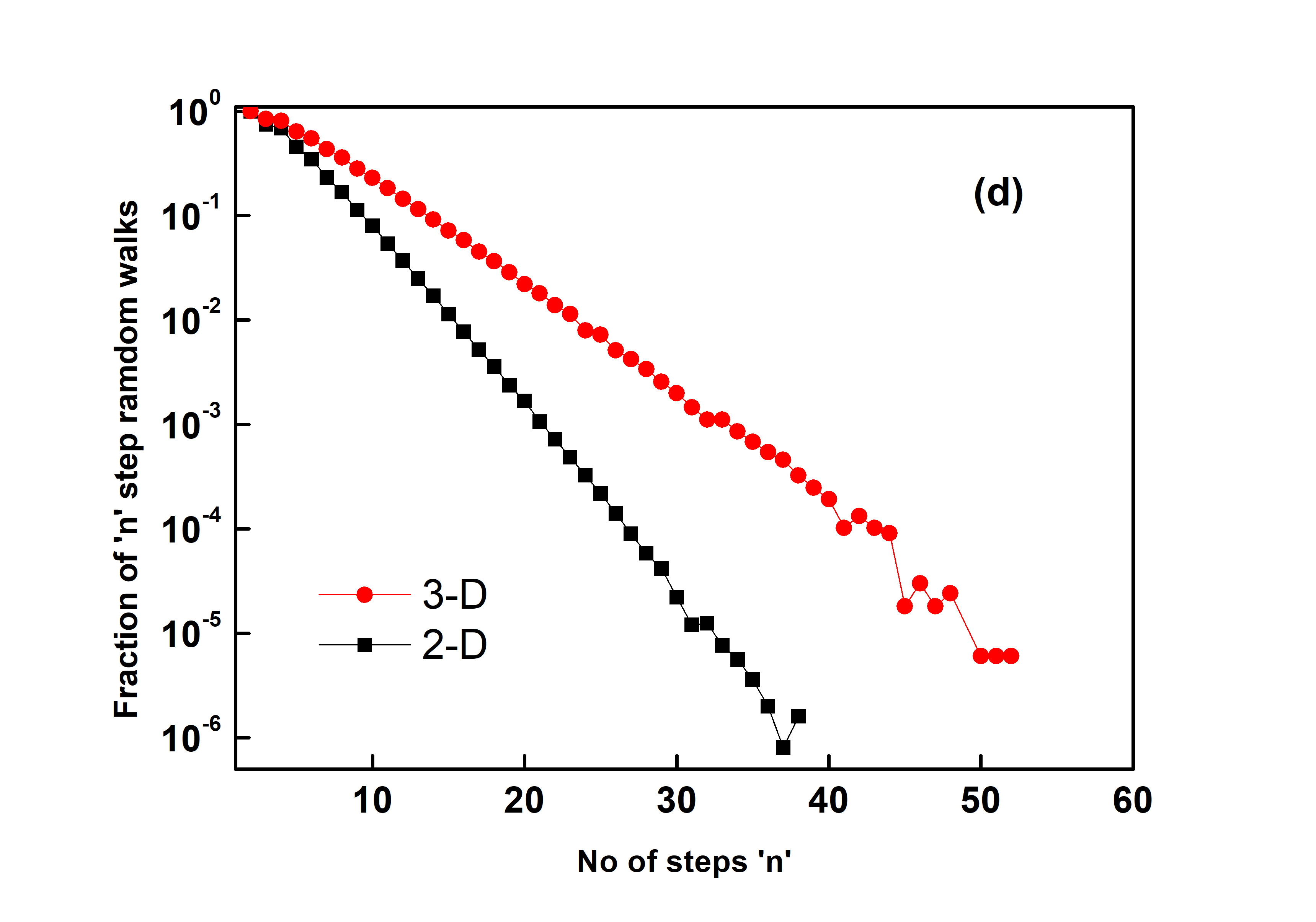
In 2-D and 3-D, we connect each site with only one neighbor. This neighbor is affected by only one neighbor and so on. This can be viewed as a random walk. Thus if we start this walk from a site that does not affect any other site and continue till the walker backtracks or gets connected to a site visited previously, the walk ends there since each site couples to only one site. A few examples of such walks are shown in Fig.4(a),(b), and (c). The fraction of such surviving walks goes down exponentially in 2-D as well as 3-D, though the exponent is smaller in 3-D.(See Fig.4(d)) Now if all the sites covered by this walk go to zero, these sites will be in an absorbing state forever since all the sites which they are affected by being in an absorbing state. These sites form a 1-D lattice of finite size in all practical senses. This leads to fragmentation of lattice and the mechanism in higher dimensions could be the same as in one dimension.

Now the question is what is the origin of the complex exponents? In the case of the 1-D model, we simulate systems of $k+2$ sites such that the first and the $k+2^{th}$ are set as inactive and the rest of the sites are kept active. Thus we have a group of $k$ sites of evolving according to rules of the 1-D model as described in the above section. For uncorrelated disorder, we expect the probability of occurance of group of a given size to decay exponentially. We denote the average time taken by this group to become inactive by $T_{k}$. We note that the fraction of groups of size $k$ surviving till time $t$ seems to be a function of $t/T_{k}$ (See Fig.5) Thus $T_{k}$ is a characteristic time for system size $k$. This average time $T_{k}$ increases exponentially with relation $T_{k}\sim\exp(\gamma k)$ with oscillations imposed over and above the exponential (See Fig6(a)). (In Fig6(b), we plot $T_{k}/\exp(\gamma_{p}k)$ versus $k$ for various values of $p$.) We argue that the combination of exponentially rare regions which survive for exponentially long times leads to a power law and the oscillations over and above this exponential leads to log-periodicity.

The standard explanation of Griffiths phase goes as follows. The probability of finding rare regions is exponentially small $P(x)\propto\exp(-cx)$ but can exhibit exponentially large lifetime $\tau(x)=\tau_{0}(x)=\exp(bx)$. The fraction of active sites can be approximated by $\rho(t)\sim\int$ $xP(x)\exp{(-t/\tau(x))}dx$. Using saddle-point approximation, it can be shown that this leads to algebraic decay of $\rho(t)$, i.e. $\rho(t)\sim t^{-c/b}$ with continuously varying exponent. We do not exactly know the functional form of relaxation times for different sizes. However, in this model, the oscillations get damped, and we propose a functional form as $\tau(x)\sim\tau_{0}(x)\tau_{p}(x)$ where $\tau_{p}(x)=\exp(-d\frac{\cos(\pi x)}{\sqrt{x}})$ because the odd-even oscillations get damped quickly. (Sign of $d$ in the expression of $\tau_{p}(x)$ does not matter because $\cos$ takes either sign.) We numerically compute the above sum $\rho(t)=\sum_{x=1}^{N}x\exp(-cx)\exp(-t\exp(-bx+d\frac{\cos(\pi x)}{\sqrt{x}}))$ for large $N$, i.e $N=10^{7}$. The plot of $\rho(t)t^{\delta^{\prime}}$ vs time clearly shows log periodic oscillations as shown in Fig.7(a). The values of $\delta^{\prime}$ and $\delta^{\prime\prime}$ do not depend on $d$ as shown in Fig.7(b). The obtained values of $\delta^{\prime}$ is close to $c/b$ as expected and it does not depend on $d$ at all. Similarly $\delta^{\prime\prime}$ does not change for any $|d|\neq 0$. However, for smaller values of $|d|$, the amplitude of oscillations is reduced and the onset of oscillations is delayed. Both exponents vary linearly with $\frac{c}{b}$ and are expected to vary linearly with each other. Although $\tau(x)$ is not a perfect analogy of the model presented here, the above simulations show that the lifetime of rare region imposed with the periodic term can generate log periodic oscillations. The exponents $\delta^{\prime}$ and $\delta^{\prime\prime}$ have a linear relationship in exponents computed using this ansatz as well as in our model. This linear variation is shown in Fig.8. The onset of oscillations is delayed when oscillations have longer periodicity in our model. We observe it in our ansatz as well. We have studied a few different functional forms of $\tau_{p}(x)$ and they lead to log-periodic oscillations as well. Thus we believe that odd-even oscillations over and above the exponential in relaxation times are the likely reason for log-periodic oscillations.

Summary: We have studied a contact process with random asymmetric couplings in 1-3 dimensions on Domnay-Kinzel automaton. In one-dimension, we study a system in which each lattice site is coupled to two neighbors either on left or on right. In two and three dimensions each site is coupled to a neighbor chosen randomly. This is a quenched disorder. For low values of $p$ the fraction of active sites $\rho(t)$ decays exponentially or stretched exponentially. But for $p\rightarrow 1$, $\rho(t)$ shows a power law decay with a complex exponent. Thus we observe log-periodic oscillations in time over and above the power law decay. This power law decay of order parameter with complex exponent can be termed as a complex Griffiths phase. Such a transition is not observed when the lattice is not effectively fragmented in disjoint units. We have also given an argument that this is likely an effect of odd-even oscillations in relaxation times as a function of size.

In the complex Griffiths phase, the real part of the exponent decreases continuously while amplitude and wavelength of oscillations increases as $p\rightarrow 1$. This is a system with a parallel update of all sites. It can be of interest to study the impact of changes in updating schemes, dimensionality, and other factors in the complex Griffiths phase.

Acknowledgement PMG thanks DST-SERB (EMR/2016/006685) for funding and Professor P. Sen and Professor M. Burma for discussions.

References

- Henkel et al. (2008) M. Henkel, H. Hinrichsen, S. Lübeck, and M. Pleimling, Non-equilibrium phase transitions, Vol. 1 (Springer, 2008).
- Rupp et al. (2003) P. Rupp, R. Richter, and I. Rehberg, Critical exponents of directed percolation measured in spatiotemporal intermittency, Phys. Rev. E 67, 036209 (2003).
- Takeuchi et al. (2007) K. A. Takeuchi, M. Kuroda, H. Chaté, and M. Sano, Directed percolation criticality in turbulent liquid crystals, Phys. Rev. Lett. 99, 234503 (2007).
- Vojta (2006) T. Vojta, Rare region effects at classical, quantum and nonequilibrium phase transitions, J. Phys. A 39, R143 (2006).
- Webman et al. (1998) I. Webman, D. Ben Avraham, A. Cohen, and S. Havlin, Dynamical phase transitions in a random environment, Philos. Mag. B 77, 1401 (1998).
- Harris (1974) A. B. Harris, Effect of random defects on the critical behaviour of ising models, J. Phys. C 7, 1671 (1974).
- Griffiths (1969) R. B. Griffiths, Nonanalytic behavior above the critical point in a random ising ferromagnet, Phys. Rev. Lett. 23, 17 (1969).
- Vojta (2003) T. Vojta, Disorder-induced rounding of certain quantum phase transitions, Phys. Rev. Lett. 90, 107202 (2003).
- Sornette (1998) D. Sornette, Discrete-scale invariance and complex dimensions, Phys. Rep. 297, 239 (1998).
- Kapitulnik et al. (1983) A. Kapitulnik, A. Aharony, G. Deutscher, and D. Stauffer, Self similarity and correlations in percolation, J. Phys. A 16, L269 (1983).
- Meurice et al. (1995) Y. Meurice, G. Ordaz, and V. G. J. Rodgers, Evidence for complex subleading exponents from the high-temperature expansion of dyson’s hierarchical ising model, Phys. Rev. Lett. 75, 4555 (1995).
- Ódor (2013a) G. Ódor, Slow dynamics of the contact process on complex networks, in EPJ Web of Conferences, Vol. 44 (EDP Sciences, 2013) p. 04005.
- Ódor (2013b) G. Ódor, Spectral analysis and slow spreading dynamics on complex networks, Phys. Rev. E 88, 032109 (2013b).
- Bhoyar and Gade (2020) P. D. Bhoyar and P. M. Gade, Dynamic phase transition in the contact process with spatial disorder: Griffiths phase and complex persistence exponents, Phys. Rev. E 101, 022128 (2020).
- Bernasconi and Schneider (1983) J. Bernasconi and W. Schneider, Diffusion in random one-dimensional systems, J. Stat. Phys. 30, 355 (1983).
- Muñoz et al. (2010) M. A. Muñoz, R. Juhász, C. Castellano, and G. Ódor, Griffiths phases on complex networks, Phys. Rev. Lett. 105, 128701 (2010).
- Cohen et al. (2000) R. Cohen, K. Erez, D. ben Avraham, and S. Havlin, Resilience of the internet to random breakdowns, Phys. Rev. Lett. 85, 4626 (2000).
- Cohen et al. (2001) R. Cohen, K. Erez, D. ben Avraham, and S. Havlin, Breakdown of the internet under intentional attack, Phys. Rev. Lett. 86, 3682 (2001).
- Wang et al. (2017) Y. Wang, J. Cao, A. Alsaedi, and T. Hayat, The spreading dynamics of sexually transmitted diseases with birth and death on heterogeneous networks, J. Stat. Mech.: Theory Exp 2017, 023502 (2017).
- Grassberger (1982) P. Grassberger, On phase transitions in schlögl’s second model, Z. Phys. B 47, 365 (1982).
- Janssen (1981) H.-K. Janssen, On the nonequilibrium phase transition in reaction-diffusion systems with an absorbing stationary state, Z. Phys. B 42, 151 (1981).
- Grassberger (1995) P. Grassberger, Are damage spreading transitions generically in the universality class of directed percolation, Journal of statistical physics 79, 13 (1995).
- Domany and Kinzel (1984) E. Domany and W. Kinzel, Equivalence of cellular automata to ising models and directed percolation, Phys. Rev. Lett. 53, 311 (1984).