Nonlinear electrodynamics at cylindrical “cumulation” fronts
Abstract
Converging cylindrical electromagnetic fields in vacuum have been shown (E.I. Zababakhin, M.N. Nechaev, Soviet Physics JETP, 6, 345 (1958)) to exhibit amplitude “cumulation”. It was found that the amplitude of self-similar waves increases without bounds at finite distances from the axis on the front of the fields reflected from the cylindrical axis. In the present paper we propose to exploit this cylindrical cumulation process as a possible new path towards the generation of ultra-strong electromagnetic fields where nonlinear quantum electrodynamics (QED) effects come into play. We show that these effects, as described in the long wave-length limit within the framework of the Euler Heisenberg Lagrangian, induce a radius-dependent reduction of the propagation speed of the cumulation front. Furthermore we compute the - pair production rate at the cumulation front and show that the total number of pairs that are generated scales as the sixth power of the field amplitude.
Keywords:
Ultraintense electromagnetic fields and Amplitude cumulation and Quantum ElectrodynamicsI Introduction
As mentioned in Ref. peg the “recent developments in the generation of laser pulses with
ultra-high power (presently petawatt and progressing) have opened up a new frontier in plasma research by making
it possible to obtain and to study “mesoscopic” amounts of
relativistic (ionised) matter in compact-size experiments in the laboratory.
This will make it possible to investigate
in a controlled environment the nonlinear dynamics
of collective relativistic systems, to enter the Quantum Electrodynamics plasma regime, and to explore conditions that are of
interest for high energy astrophysics and beyond.”
On the other hand,
in the presence of ultra-intense electromagnetic fields that approach the scale of the so called Schwinger field, i.e. of the electric field that corresponds to an energy gain on a Compton length equal to the electron mass energy, vacuum itself behaves as a nonlinear medium where the electromagnetic waves induce polarisation and magnetisation currents.
As recalled e.g. in Ref. hod in “classical electrodynamics electromagnetic waves do not interact in vacuum. On the contrary, in QED photon-photon scattering can take
place in vacuum via the generation of virtual electron-positron pairs. This interaction gives rise to vacuum polarisation and birefringence,
to the Lamb shift, to a modification of the Coulomb field, and to many other phenomena BLP” (see Refs.piazza; king; rend).
The electromagnetic fields in present laser pulses do not approach the magnitude of the Schwinger field ( where the symbols have their standard meaning), but the nonlinear properties of relativistic plasmas, and in particular the so called relativistic flying mirrors bulan; MTB; BEK; BulR can be used to significantly enhance and focus the electromagnetic energy of presently available laser pulses. As noted in atto, “the measurement and control of sub-cycle field evolution of few-cycle light have opened the door to a radically new approach to exploring and controlling processes of the microcosm.”
An alternative approach is to search for geometrical configurations and pulse shapes that can lead to a local enhancement of the pulse field intensity through the process of amplitude cumulation, i.e. to a local formal divergence of the field intensity through a mechanism of constructive interference. In fact, converging cylindrical electromagnetic fields in vacuum have been shown cumul to exhibit amplitude cumulation. It was found that the amplitude of self-similar waves increases without bounds at finite distances from the axis on the front of the fields reflected from the cylindrical axis. It was remarked that this cumulation process is a different phenomenon with respect to the dependence close to the cylinder axis, being the distance from the axis, that follows simply from the Poynting flux conservation in a cylindrical configuration. The amplitude cumulation is produced by the constructive interference that is induced because the self-similar electromagnetic pulse has a fully coherent spectrum which extends over the whole frequency range and decays for large frequencies as the inverse of the frequency square-root.The effects of the pulse geometry and coherence combine in such a way that after the reflection from the cylindrical axis a wave front is formed that propagates outwards at the speed of light. At this front the field amplitude formally diverges. In Ref. cumul the important fact that this singularity is not limited to the axis but sweeps a wide area was emphasised.
An obvious problem when applying the amplitude cumulation mechanism to the creation of ultra intense electromagnetic fields arises as to how such a self-similar pulse can be prepared and how stable it is to small deviations in its spectral composition and in its phase coherence. In Ref.cumul the point was made that a self-similar solution of the Maxwell’s equations “describes the limiting behaviour of a field close to the axis and close to the time of focusing”. On the other hand, in the context of the implosion of cylindrical liners, this idealised solution has been explicitly criticised in Ref.critic on the point that it does not satisfy the “the boundary condition imposed by magnetic flux conservation for field compression by an ideally conducting cylinder”, i.e. for the configuration for which it was initially constructed.
In the present paper we do not directly address these points but exploit the fact that in a cylindrical electromagnetic wave the Lorentz invariant (also known as the Poincaré invariant of the electromagnetic field) does not vanish, as would be the case for plane electromagnetic waves. This fact, together with the large fields produced at the cumulation front, can make this configuration interesting for the study of QED effects in vacuum within the framework described by the Euler-Heisenberg EH Lagrangian. In fact a converging cylindrical configuration can be seen as a limiting case combining the converging multi-light-beam approach adopted e.g. in Ref.bulanino and, in view of the reflection at the magnetic axis, the counter propagating laser pulse approach (for a recent investigation of this latter approach see Ref. hod). Similarly, these combined effects can be exploited in order to enhance the production of - pairs at the cumulation front.
This article is organised as follows. In Sec.II the reduced Lagrangian densities for - and for -polarised fields in cylindrical geometry are derived from the general electromagnetic vacuum action functional that includes the long wave-length QED corrections to classical electrodynamics. In Sec.III the classical limit is considered and the self-similar solutions are explicitly constructed and found to involve Elliptic integrals of the self-similar variable . It is shown that at the cumulation front both the electromagnetic fields and the Lorentz invariants diverge logarithmically. The spectrum of the self-similar solutions is computed and shown to decay as the inverse square root of the frequency for large frequencies. In Sec.IV the QED corrections are computed explicitly for the -polarised electromagnetic fields and interpreted in terms of a reduction of the wave propagation speed. In Sec.V the production rate of electron-positron pairs in the region near the cumulation front and the total number of pairs created by a self-similar pulse are computed. Finally, in Sec.VI we formulate our conclusions.
II Euler Heisenberg Lagrangian density
In the long wave-length limit the electromagnetic action functional in vacuum that includes the QED corrections EH; BLP to classical electrodynamics can be expressed as
| (1) |
where
| (2) |
is the Lagrangian density of classical electrodynamics in vacuum and is the Heisenberg–Euler Lagrangian density. Here is the electromagnetic field tensor
| (3) |
with the 4-vector of the electromagnetic field and . Here and below we assume summation over repeated indices and adopt natural units setting .
In the weak field approximation (see e.g. HeHe) the Heisenberg–Euler Lagrangian density can be written as
| (4) |
with and and the Poincaré invariants
| (5) |
and is the dual electromagnetic tensor with the Levi-Civita symbol in four dimensions. In the above equations, and in the following sections unless explicitly stated, the electromagnetic fields are normalised on the Schwinger field. In the Lagrangian density (4) the first two terms on the right hand side and the last two correspond respectively to four and to six photon interaction, respectively. In the following, for the sake of simplicity, we will retain only the four photon interaction term.
II.1 Cylindrical waves
Here we address the propagation of converging cylindrical electromagnetic waves with either -type or -type polarisation. We will consider the two polarisations separately, aside for Sec.(III) where the cylindrical wave equations are derived by neglecting the Euler-Heisenberg correction to the classical Lagrangian density and thus obey the superposition principle. This simply amounts to a simplification of the analysis as in this case the invariant that would couple the two polarisations in the Euler-Heisenberg Lagrangian density vanishes identically. In physical terms this amounts to including the effect of photon-photon scattering while disregarding the effect of vacuum induced birefringence. Furthermore we assume translational invariance along , i.e. along the axis direction, and azimuthal invariance along the angle .
The -type waves can be described in a transverse gauge by a vector potential with a single component, , where is the unit vector along the axis. Similarly, the -type waves can be described by a vector potential with a single component, , with the unit vector along the azimuthal direction. Factoring the two invariance directions out of the action functional, we obtain with obvious notation for the two polarisations separately
| (6) |
where
| (7) | ||||
| (8) | ||||
with where is the fine structure constant.
III Classical electrodynamics limit,
Varying the Action functional (6) with respect to the two components of the vector potential and expressing the resulting equations in the limit in terms of the electromagnetic fields, we obtain the field equations
| (9) |
for the -polarisation and
| (10) |
for the -polarisation. The two polarisations are related by the symmetry transformation and which is characteristic of classical electrodynamics in vacuum. Eqs.(9, 10) lead to the cylindrical wave equations
| (11) |
for the -polarisation and to the corresponding one with and interchanged for the -polarisation.
III.1 Reduced fields
In cylindrical geometry it is convenient to introduce the reduced electromagnetic fields
| (12) |
where and are now dimensionless space-time coordinates normalised on a spatial reference scale . Then for the -polarisation we obtain
| (13) |
and for the -polarisation
| (14) |
From Eqs.(13,14) we obtain the reduced form of the Poynting flux and the radial electromagnetic momentum density equations for each polarisation separately
| (15) |
| (16) | ||||
In addition the mixed polarisation equations hold
| (17) | ||||
where . Note that the “source terms” in the r.h.s. of Eqs. (16) and on the second of Eqs. (17) are the terms that determine the magnitude of the Euler-Heisenberg contribution relative to the classical part in the electromagnetic Lagrangian density.
III.2 Self-similar fields
Following Ref.cumul, we look for self-similar solutions of Eqs.(13,14) by assuming that the fields and depend on the single variable . We obtain
| (18) |
We set the time origin such that corresponds to the converging part of the solution and to the diverging one. Consistently, we impose that on the converging part and have the same sign while and have opposite signs, as implied by propagation towards the cylinder axis.
In particular at (i.e. at , with ) from Eqs.(III.2) we obtain
| (19) |
Differentiating Eqs.(III.2) with respect to we obtain for the pairs and the second order ordinary differential equations
| (20) |
| (21) |
Equations (20,21) are singular at where a local analysis gives the two independent solutions in the form
| (22) |
where and are constants with the index referring to respectively and only the leading term of the local expansions is shown.
In the following we require that the converging part of the solution for the electromagnetic fields be regular and thus set , i.e. we impose that the solution have no logarithmic singularity at .
Equations (20,21) are Legendre equations of index and respectively. Following Ref.NIST we write their solutions in the interval in terms of elliptic integrals as
| (23) | ||||
where are Legendre functions (see Ref.NIST) and and are complete elliptic integrals of the first and second kind, respectively. In accordance with the regularity condition at , in Eqs.(23)
we have imposed .
For the solutions (23) display a logarithmic singularity as while .
The solutions of Eqs.(20,21) in the interval that vanish for , i.e. that vanish on the cylinder axis, can be written as
| (24) |
where are Legendre functions NIST and the coefficient has been fixed by requiring that the electromagnetic fields be continuous at .
Note in passing that, when inserted into Eqs.(12) these solutions lead to electric and magnetic fields that are regular at for and that depend on time as .
The expressions for the magnetic field components and are obtained by inserting for and for in Eqs.(23,III.2).
The logarithmic singularity at corresponds to the cumulation process first identified in Ref.cumul. It occurs at a finite distance from the axis, at the front of the reflected fields, and propagates outwards at the speed of light.
The coefficients of the logarithmic singularity at in the electric and magnetic fields are related to each other by the leading order terms in Eqs.(III.2) and are thus either equal or equal and opposite. However, for each of the polarisation, the next order terms for the electric and magnetic field expansion differ: thus in the terms and the contributions
proportional to the logarithm squared cancel out while the linear ones in the logarithm do not.
More explicitly for from Eqs.(23), using the relationships between and and between and mentioned above, and setting and , we find
| (25) |
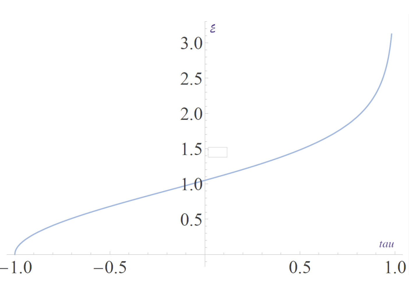
which diverges as for see Fig.(1) Note the opposite sign of the invariants in Eq.(III.2) between the and the polarisations.
Corresponding formulae can be obtained from Eqs.(III.2) for .
The cancellation of the leading order terms in the Lorentz invariants ,
and can be also seen without resorting to the explicit solutions (23,III.2) by rewriting Eqs.(15, 16) in terms of the self-similar fields. We obtain
| (26) | ||||
with for the polarisation and for the -polarisation, which give for both polarisations the following equation for the reduced Poynting flux
| (27) |
Similarly from Eqs.(17) we obtain for the mixed polarisation case
| (28) | ||||
which give
| (29) |
Inserting the local expansion (22) into Eqs.(27,29), in the neighbourhood of we recover .
III.3 Frequency spectrum of the self-similar fields
Let us consider the cylindrical wave equations (11) with
| (30) |
Then
| (31) |
We write (and analogously for ) in the form
| (32) |
where denotes a combination, depending on the initial conditions, of Bessel functions of index . Then Eqs.(30,32) together with the self-similarity condition can be written (in dimensional units) as
| (33) |
i.e.,
| (34) |
Consistency between the r.h.s. and the l.h.s. of Eq.(34) requires that
| (35) |
which corresponds to a slow decay of the frequency spectrum for with all the frequency components being in phase.
We observe that the singularity at can be re-derived by inserting the large behaviour of the Hankel function
of the first kind for into the integrand in Eq.(34) and by evaluating the integral explicitly.
This procedure allows us to compute the modification of the logarithmic singularity if we impose a cut-off in the frequency spectrum while preserving the spectrum coherence. If, for example, we impose a Gaussian cut-off by modifying Eq.(35) and setting
| (36) |
we find that .
IV QED corrections to the propagation of the cumulation front
Varying the Action functional (6) with respect to the two components of the vector potential separately and expressing the resulting equations in terms of the electromagnetic fields, we obtain for the field equations
| (37) |
for the -polarisation and for the -polarisation
| (38) |
In the following we will examine the effect of the Euler-Heisenberg corrections on the self-similar solutions described in Sec.III.2 by adopting a perturbative procedure in , where the additional geometrical factor accounts for the fact that the nonlinear terms grow as in comparison with the linear terms as the cylinder axis is approached. Furthermore, in order not to duplicate the derivation, we will only refer explicitly to the polarised case. Following Eq.(12), we use the reduced fields and which we expand as
| (39) |
where and are given by Eqs.(23, III.2) with . Then to first order in we obtain
| (40) | ||||
where a common factor as been removed. Equations (40) can be recast in the form
| (41) |
to be solved in the domain . Here
| (42) |
In order to limit the number of required algebraic manipulations, in the following it will suffice to present the solutions of Eq.(IV) explicitly only in the interval , i.e. in front of the cumulation singularity.
Using the expressions in in Eqs.(23) we find, see Fig.(2),
| (43) | ||||
which diverges as as .

Similarly to Eqs.(20), the differential operators in Eqs.(IV) are singular at . The homogeneous solutions of Eq.(IV) for the electric field can be expressed as a linear combination of and with
| (44) | ||||
which diverge at as , respectively.
Analogously, the homogeneous solutions of Eq.(IV) for the magnetic field can be expressed as a linear combination of and
| (45) | ||||
The inhomogeneous term is singular at . At the first two terms in Eq.(42) combine to give a contribution proportional to that, according to Eq.(23) and accounting for cancellations, diverges as The third term in Eq.(42) diverges as . The solution of Eq.(IV) that is initialised at can be obtained with the general method of the variation of the constants, in the form
| (46) | ||||
where
| (47) |
is the Wronskian of the two independent homogeneous solutions
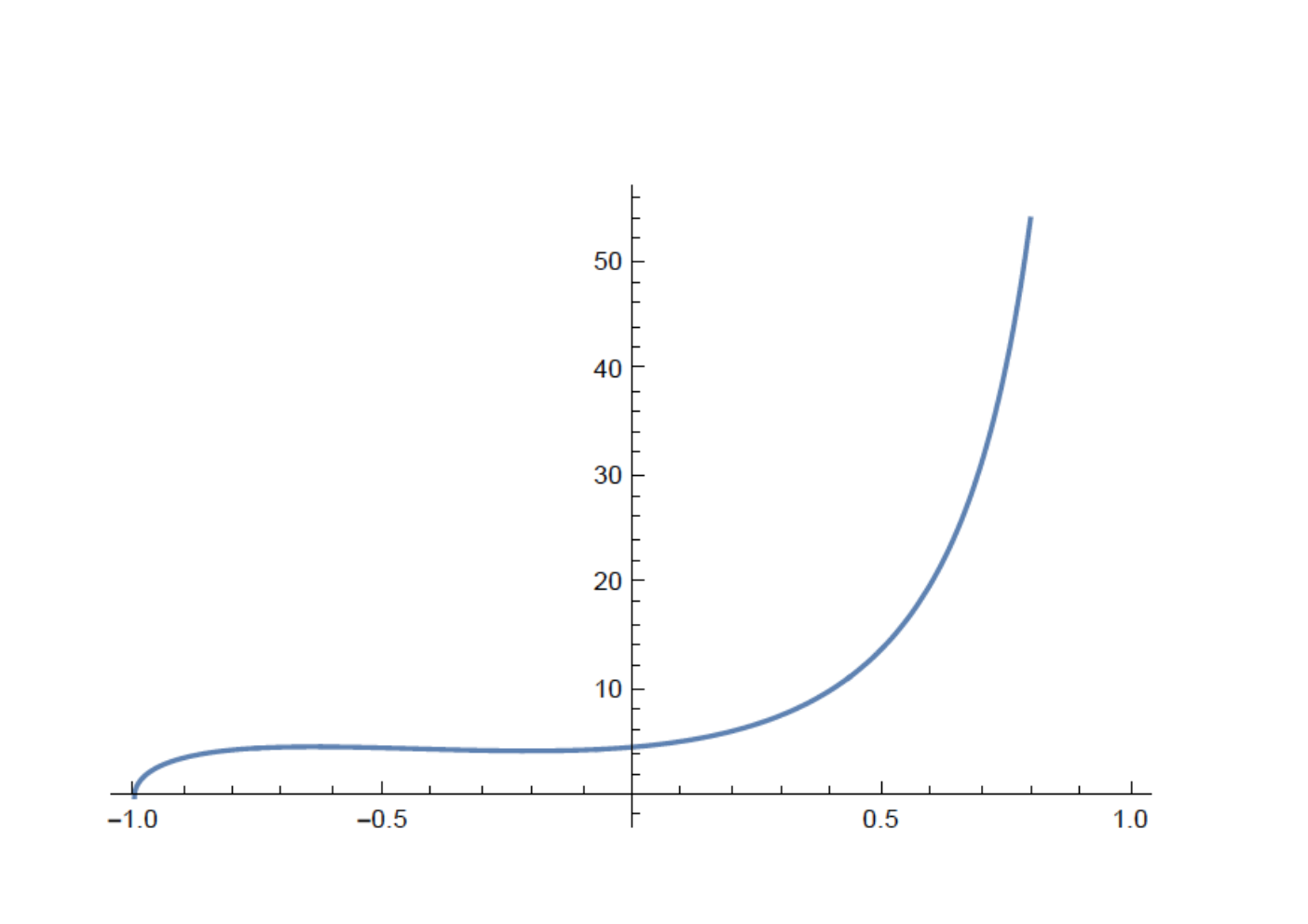

Consistently with a local analysis based on Eqs.(IV,43), Fig.(4) shows that diverges proportionally to as . Although formally the perturbation procedure breaks down at the singularity, the above result can be easily reinterpreted by observing that the nonlinear interaction between the converging and the diverging portions of the electromagnetic radiation makes the radiation propagate at a speed smaller than the speed of light (see e.g. Ref.Gies). This velocity reduction depends on the field intensity. It is thus proportional to the expansion parameter used in Eq.(39) and leads to an -dependent shift, for given , of the position of the cumulation front. A similar shift was noted in Ref hod in the case of self-similar, counter-propagating waves in a Cartesian geometry. The expansion of the logarithmic singularity around the unperturbed cumulation front leads to the divergent correction found above. We note that, following the approach of Ref.hod this result could have been derived more consistently by using a renormalised expansion procedure where a counter term is added to the leading order terms so as to make the first order correction finite, i.e. by setting
| (48) |
and by solving for so as to cancel the term in that leads to the singularity.
V Generation of electron positron pairs
Two features of the self-similar converging and diverging electromagnetic fields in a cylindrical configuration can be exploited for enhancing the production of electron positron pairs. First, as is the case for converging and focussed beams bulanino, the Lorentz invariant does not vanish and, as shown by Eq.(III.2), it is positive for the -polarisation i.e. for the case where the electric field is parallel to the cylinder axis while the magnetic field is azimuthal. In addition, at the cumulation front diverges logarithmically, thus formally exceeding the Schwinger field . On the other hand the width of enhanced field region is relatively narrow so that the pair production region will appear, at fixed , as a thin expanding ring.
For purely -polarised fields the Lorentz invariant vanishes identically and the pair production rate (see Ref. BLP) is given
in dimensional units by
| (49) |
where is the invariant electric field . For the -polarisation the invariant electric field in the interval normalised on the Schwinger field is given by
| (50) |
where the factor arises from the field representation in Eq.(12). A corresponding expression applies to the interval . In Eq.(50) is dimensional while the amplitude has the dimension of the square root of a length, unlike from Eq.(III.2) where it is dimensionless. Inserting Eq.(50) into the volume integral in Eq.(49) in cylindrical coordinates we find
| (51) |
At fixed time , the dominant contribution to the radial integral arises from the neighbourhood of where with . Thus, taking into account the two sides of the logarithmic singularity (and using the continuity of the electromagnetic fields at ) we can rewrite the r.h.s. of Eq.(51) as
| (52) |
where and the precise determination of the upper limit of integration is not needed since the integrand is strongly localised around for most cases of interest. Thus the pair production rate in Eq.(49) for the self-similar cylindrical -polarised configuration can be written per unit length along in the form
| (53) | ||||
where . The integral on the r.h.s. of Eq.(53) decreases extremely rapidly as decreases. The plot of minus the logarithm of as a function of in Fig. 5 shows the rapid decrease of the pair production rate with decreasing field amplitudes.

The total number of electron-positron pairs per unit length along generated at the cumulation front by a self-similar pulse initialised at can be estimated by taking the integral over time in Eq.(53) first and then by performing the integral over . Using the relationship we obtain
| (54) |
Then, taking and using we find
| (55) |
While the exact value of the numerical coefficient can be affected by the approximations made in its calculation, the dependence on can be understood simply from first principles. First we observe that the number of electron-positron pairs per unit length has the dimension of an inverse length while is the inverse of the reduced Compton length . By definition a self-similar configuration cannot provide an intrinsic scale-length to be used in the definition of the volume that is needed to balance Eq.(55) dimensionally. However a spatial scale can be derived from the behaviour of the electromagnetic fields in a cylindrical configuration as given by Eq.(12). In fact the amplitude has the dimension of the square root of a length and can be read as the radial distance from the axis where the electric field amplitude is equal to the Schwinger field. Thus Eq.(55) can be interpreted by saying that the number of pairs produced in a disc of height along equal to is given by a numerical coefficient of order unity times the cube of the ratio .
VI Conclusions
In this article we have analysed two QED effects on a properly arranged, cylindrical, electromagnetic configuration, with a high degree of spectral coherence, that develops an expanding cumulation front where the electromagnetic fields diverge logarithmically. We have shown that QED effects make the reflected cumulation front expand with a velocity smaller than the speed of light, similarly to what is known to occur when two counter-propagating electromagnetic pulses interact nonlinearly. We have computed the effect of the enhancement of the electromagnetic fields at the expanding front on the production rate of electron-positron pairs. We have shown that the total number of pairs produced scales as the sixth power of the electromagnetic field amplitude.
The analysis presented above is not exhaustive in several aspects. One concerns the realisability in the laboratory of the highly coherent fields that lead to the cumulation process and the assessment of the resilience of the cumulation mechanism to errors in the field generation. Moreover it may not be fully consistent to use the Euler Heisenberg Lagrangian, which is derived in the long wavelength limit, to account for the QED effect too close to the cumulation front where the local gradient of the field amplitude diverges as .
Two obvious problems arise from the slow decay of the frequency spectrum as and from the proper boundary conditions to be imposed to a “local” realisation of the self-similar solution in order to obtain a finite duration pulse.We have shown that, if we impose e.g. a frequency Gaussian cut-off with width in the frequency spectrum while preserving the spectrum coherence, the amplitude cumulation turns out to be bounded and that the logarithmic singularity at is changed into .
Regarding the pulse duration, a finite pulse that exhibits amplitude cumulation, although transiently in time, can be obtained by considering a “truncated” self-similar solution. In the derivation in Sec.III.2 the self-similar fields are initiated at that is for all values of and, for each , at the corresponding past time . We may consider instead a truncated self-similar solution, that is a solution that is initiated at but extends only on a finite interval, and thus on a finite interval.
Since all parts of the self-similar solutions propagate at the same speed of light causality requires that this “truncated ” part of the self-similar solution propagates at and if it is sufficiently long, i.e. more than two times the distance from the cylinder axis, for a finite time interval it will not suffer from the fact that portion of the self-similar solutions are missing leading to a transient cumulation front. Clearly this condition must be satisfied in the interval where the constructive interference with the reflected pulse can occur which can substantially reduce the portion of the truncated pulse that can be used for building the transient cumulation front, thus reducing the efficiency of the process.
The formation of the singularity during the cumulation of a strong electromagnetic wave formally assumes that the frequency spectrum of the wave does not decay exponentially when the frequency tends to infinity, as discussed above. The counter-play between the electromagnetic field intensification and the wave steepening at the singularity may result either in stronger electron-positron pair generation by the Schwinger effect, as considered above, or in the creation of a pair plasma because the Breit-Wheeler mechanism becomes dominant (see the review article piazza and references therein) and/or in the modification of the singularity due to dispersion effects.
We note that the frequency spectrum of the electromagnetic wave can be determined not only by the boundary conditions but also by the high order harmonics generated in the nonlinear vacuum. These high order harmonics are a manifestation of nonlinear processes and have attracted a lot of attention in theoretical articles devoted to the study of the QED vacuum DHK-2005; BKR-2015; FN-2007; KKB-2019; SEPB-2020. The harmonic development can modify the singularity formed in the QED vacuum. In combination with the dispersion effects, the counter-play between nonlinearity and dispersion can result in the formation of solitons BSPKBER-2020. This regime is beyond the scope of the present work and will be addressed in a future paper.
We conclude by stating that, notwithstanding these limitations, our analysis indicates that it may be worthwhile to reconsider, e.g. in a three-dimensional configuration, the process of amplitude cumulatiosn described in a cylindrical geometry in Ref.cumul as it may represent a promising new approach to the study of QED effects in the laboratory.
Acknowledgements
S.V.B. acknowledges the support by the project High Field Initiative
(CZ.02.1.01/0.0/0.0/15_003/0000449) from the European Regional Development Fund.
F.P. would like to acknowledge the hospitality of the ELI-Beamlines Project, Na Slovance 2, 182 21 Prague, Czech Republic.
References
- (1) F. Pegoraro, Plasmas in extreme electromagnetic fields, Rend. Fis. Acc. Lincei, 30, 11 (2019).
- (2) F. Pegoraro, S.V. Bulanov, Hodograph solutions of the wave equation of nonlinear electrodynamics in the quantum vacuum, Phys. Rev. D, 100, 036004 (2019).
- (3) V.B. Berestetskii, E.M. Lifshitz, L.P. Pitaevskii, in Quantum Electrodynamics, (Pergamon, New York, 1982).
- (4) A. Di Piazza, C. Müller, K.Z. Hatsagortsyan, C.H. Keitel, Extremely high-intensity laser interactions with fundamental quantum systems, Rev. Mod. Phys., 84, 1177 (2012).
- (5) B. King, T. Heinzl, Measuring vacuum polarization with high-power lasers, High Power Laser Science and Engineering, 4, e5 (2016).
- (6) A. Angioi, A. Di Piazza, On quantum electrodynamic processes in plasmas interacting with strong lasers, Rend. Fis. Acc. Lincei, 30, 17 (2019).
- (7) S.V. Bulanov, T. Esirkepov, T. Tajima, Light Intensification towards the Schwinger Limit, Phys. Rev. Lett., 91, 085001 (2003).
- (8) G. Mourou, T. Tajima, S. V. Bulanov, Optics in the relativistic regime, Rev. Mod. Phys., 78, 309 (2006).
- (9) S.V. Bulanov, T.Zh. Esirkepov, M. Kando, A.S. Pirozhkov, N.N. Rosanov, Relativistic Mirrors in Plasmas–Novel Results and Perspectives, Physics Uspekhi, 56, 429 (2013).
- (10) S.V. Bulanov, Dynamics of relativistic laser-produced plasmas, Rend. Fis. Acc. Lincei, 30, 5 (2019).
- (11) F. Krausz, M. Ivanov, Attosecond physics, Rev. Mod. Phys., 81, 163 (2009).
- (12) E. I. Zababakhin, M. N. Nechaev, Electromagnetic-field shock waves and their cumulation, Soviet Physics JETP, 6, 345 (1958).
- (13) H. E. Wilhelm, Hyperbolic theory of electromagnetic cumulation in cylindrical liner implosions, Phys. Rev. A, 27, 1515 (1983).
- (14) W. Heisenberg, H. Euler, Folgerungen aus der Diracschen Theorie des Positrons, Z. Phys., 98, 714 (1936).
- (15) S. S. Bulanov, V. D. Mur, N. B. Narozhny, J. Nees, V. S. Popov, Multiple Colliding Electromagnetic Pulses: A Way to Lower the Threshold of Pair Production from Vacuum, Phys. Rev. Lett. , 104, 220404 (2010).
- (16) J. S. Heyl, L. Hernquist, Analytic form for the effective Lagrangian of QED and its application to pair production and photon splitting, Phys. Rev. D, 55, 2449 (1997).
- (17) F. W. J. Olver, D. W. Lozier, R. F. Boisvert, C. W. Clark, eds. NIST Handbook of Mathematical Functions. National Institute of Standards and Technology (NIST), (U.S. Department of Commerce, Cambridge University Press, 2010), https://dlmf.nist.gov/19.6.
- (18) W. Dittrich, H. Gies, Springer Tracts Mod. Phys., 166, 1 (2000).
- (19) A. Di Piazza, K.Z. Hatsagortsyan, C. H. Keitel, Harmonic generation from laser-driven vacuum, Phys. Rev. D, 72, 085005 (2005).
- (20) P. Böhl, B. King, H. Ruhl, Vacuum high-harmonic generation in the shock regime, Phys. Rev. A, 92, 032115 (2015).
- (21) A.M. Fedotov, N.B. Narozhny, Generation of harmonics by a focused laser beam in the vacuum, Phys. Lett. A, 362, 1 (2007).
- (22) H. Kadlecova, G. Korn, S. V. Bulanov, Electromagnetic shocks in the quantum vacuum, Phys. Rev. D, 99, 036002 (2019).
- (23) P.V. Sasorov, T.Zh. Esirkepov, F. Pegoraro, S.V. Bulanov, Harmonics in quantum vacuum, in preparation.
- (24) S.V. Bulanov, P.V. Sasorov, F. Pegoraro, H. Kadlecova, S.S. Bulanov, T.Zh. Esirkepov, N.N. Rosanov, G. Korn, Electromagnetic Solitons in Quantum Vacuum, Phys. Rev. D, 101, 016016 (2020).