Two-level quantum Otto heat engine operating with unit efficiency far from the quasi-static regime under a squeezed reservoir

Classical heat engines convert thermal resources into work, which is maximized for reversible operations where the entropy production vanishes. In the quantum realm, both the engine and the reservoirs can be composed of finite-dimensional systems Kieu 2004; Quan et al. 2007; Wang et al. 2009; Linden et al. 2010; Scully et al. 2011; Wang et al. 2012; Rahav et al. 2012; Gelbwaser-Klimovsky et al. 2013; Uzdin et al. 2015; Kosloff and Rezek 2017; Huang et al. 2017; Zhao and Zhang 2017; Brandner et al. 2017; Niedenzu et al. 2018; Dorfman et al. 2018; Camati et al. 2019; Türkpençe and Altintas 2019; Peterson et al. 2019; Bera et al. 2019; Çakmak and Altintas 2020, thus departing from classical scenarios. Differently from the classical case, quantum engines, as well as their environments, can be prepared in physical states without classical analogues, allowing the efficiency to be strongly enhanced Roßnagel et al. 2014; Manzano et al. 2016; Klaers et al. 2017; de Assis et al. 2019. For cyclic heat engines to be useful in the real world, it is necessary that the cycles be performed in finite time or non-null power, which introduces losses due to irreversibility. Attempts to build thermal engines operating with finite-time cycles without losing efficiency have been made. Some of these attempts consist in exploiting quantum resources such as coherence Scully et al. 2003, while others employ techniques based on the shortcut to adiabaticity Guéry-Odelin et al. 2019, which consists of changing the dynamics of the system to minimize the irreversible losses of the fast dynamics Beau et al. 2016. Yet, other approaches propose nonequilibrium reservoirs as the environment for heat engines to operate Xiao and Li 2018; de Assis et al. 2019; Wang et al. 2019; Singh and glu 2020. So far, all those proposals are mainly concerned with investigating the trade-off between efficiency and power either by trying to eliminate the irreversible losses during the finite time operation or trying to get efficiency at maximum power in the quasi-static cycle, which can be higher than Carnot efficiency Roßnagel et al. 2014. Exception to these approaches is the recent theoretical and experimental work in Ref. de Assis et al. 2019, where the authors explored reservoirs with effective negative temperatures and showed that, for a given set of parameters, the faster the processes are performed, the greater the efficiency of the engine.

In this paper we study the efficiency of a quantum Otto heat engine (QOHE) with a two-level system (TLS) as a working substance operating under a cold thermal reservoir and a squeezed hot thermal reservoir. We then explore how advantageous is to extract work both at null and at non-null power regime. By comparing our model with a similar one in which a harmonic oscillator (HO) is used as the working substance in the QOHE Roßnagel et al. 2014, we show that our model presents enhancement in the efficiency at maximum power. Here we also consider a set of QOHE parameters for a possible experimental implementation in the field of nuclear magnetic resonance (NMR).

Our model consists of a TLS as the working substance undergoing unitary operations and interacting with a cold thermal reservoir and with a squeezed hot thermal reservoir to perform a QOHE. A QOHE consists of two isochoric branches, one with the working substance coupled to the cold thermal reservoir and the other coupled to the hot thermal reservoir, and two isentropic branches, in which the working substance is disconnected from the thermal reservoirs and evolves unitarily. Inspired by recent studies on QOHEs in NMR, Refs. Peterson et al. 2019; de Assis et al. 2019, we consider here the following four-stroke QOHE:

(i) Cooling stroke. Initially, the TLS is weakly coupled to the cold thermal reservoir up to thermalization. The thermalized TLS is then described by the Gibbs state $\rho_{1}^{G}=\text{e}^{-\beta_{c}H_{c}}/\text{Tr}\left(\text{e}^{-\beta_{c}H_{c}}\right)$, where $H_{c}$ is the TLS Hamiltonian and $\beta_{c}=1/k_{B}T_{c}$, where $k_{B}$ is the Boltzmann constant and $T_{c}$ is the reservoir temperature. The Hamiltonian has the form $H_{c}=\frac{1}{2}\hbar\omega_{c}\sigma_{x}$, with $\hbar$, $\omega_{c}$, and $\sigma_{x}$ being the reduced Planck constant, the angular frequency, and the x Pauli matrix, respectively. The TLS Hamiltonian remains unchanged during the thermalization process.

(ii) Expansion stroke. In this stage, from time $t=0$ to $t=\tau$, the TLS evolves unitarily from the state $\rho_{1}^{G}$ to $\rho_{2}=U\rho_{1}^{G}U^{\dagger}$, where $U$ is the unitary operator. The unitary evolution is characterized by the driving of the TLS Hamiltonian from $H_{c}=\frac{1}{2}\hbar\omega_{c}\sigma_{x}$ to $H_{h}=\frac{1}{2}\hbar\omega_{h}\sigma_{y}$, with $\omega_{h}$ being an angular frequency greater then $\omega_{c}$ (energy gap expansion) and $\sigma_{y}$ the y Pauli matrix. Here, we are not concerned with the specific form of the unitary operator $U$.

(iii) Heating stroke. Here, the TLS is weakly coupled to the squeezed (non-equilibrium) hot thermal reservoir until reaching the stead state $\rho_{3}^{S}=S\rho_{3}^{G}S^{\dagger}$. The TLS would reach the Gibbs state $\rho_{3}^{G}=\text{e}^{-\beta_{h}H_{h}}/\text{Tr}\left(\text{e}^{-\beta_{h}H_{h}}\right)$ when thermalizing with the hot thermal reservoir without squeezing. However, reservoir squeezing changes the asymptotic state of the TLS according to operator $S=\left(\mu\left|-_{y}\right\rangle\left\langle+_{y}\right|+\nu\left|+_{y}\right\rangle\left\langle-_{y}\right|\right)/\sqrt{\mu^{2}+\nu^{2}}$, where $\mu=\cosh r$ and $\nu=\sinh r$. The state $\left|\pm_{y}\right\rangle$ is the eigenstate of $H_{h}$ with eigenenergy $\pm\frac{1}{2}\hbar\omega_{h}$, and $r$ is the squeezing parameter. The form of $\rho_{3}^{S}$ described here can be easily verified by noting its correspondence with Eq. (10) from Ref. Srikanth and Banerjee 2008. As in the cooling stroke, here the TLS Hamiltonian also remains unchanged.

(iv) Compression stroke. This stage is accomplished by reversing the protocol adopted in the above expansion stroke, such that the TLS Hamiltonian is driven from $H_{h}=\frac{1}{2}\hbar\omega_{h}\sigma_{y}$ to $H_{c}=\frac{1}{2}\hbar\omega_{c}\sigma_{x}$ and the TLS state evolves unitarily from to $\rho_{3}^{S}$ to $\rho_{4}=U^{\dagger}\rho_{3}^{S}U$.

The main quantity we are interested in is the QOHE efficiency $\eta_{TLS}$ . In the field of quantum thermodynamics, the engine efficiency is given by $\eta=-\left\langle W_{ext}\right\rangle/\left\langle Q_{abs}\right\rangle$, where $\left\langle Q_{abs}\right\rangle$ is the average total heat absorbed and $\left\langle W_{ext}\right\rangle$ is the average net work extracted from the engine. Note that $\left\langle Q_{abs}\right\rangle>0$ means energy flow into the engine, while $\left\langle W_{ext}\right\rangle<0$ means energy flow out of the engine. In order to determine the efficiency, we need to introduce the first law of thermodynamics, together with work and heat definitions. The first law of thermodynamics establishes that the change in the internal energy of a given system during a thermodynamic process can be decomposed into heat and work. In the quantum thermodynamics domain, the first law is written as $\left\langle\Delta E\right\rangle=\left\langle Q\right\rangle+\left\langle W\right\rangle$, where $\left\langle\Delta E\right\rangle$ is the average change in internal energy, which is given by $\left\langle E\right\rangle=\text{Tr}\left(\rho H\right)$. The definitions of heat and work averages we are interested in are $\left\langle Q\right\rangle=\int dt\text{Tr}\left[\left(d\rho/dt\right)H\right]$ and $\left\langle W\right\rangle=\int dt\text{Tr}\left[\rho\left(dH/dt\right)\right]$ Alicki 1979; Kosloff 1984, such that $\left\langle W\right\rangle=0$ ($\left\langle\Delta E\right\rangle=\left\langle Q\right\rangle$) in the heating and cooling strokes and $\left\langle Q\right\rangle=0$ ($\left\langle\Delta E\right\rangle=\left\langle W\right\rangle$) in the expansion and compression strokes.

We can now obtain the average heat exchanged with the reservoirs, the average net work, and then the efficiency. Thus, with the information provided in (i)-(iv) strokes, we obtain

and

where $\theta_{c\left(h\right)}=\frac{1}{2}\beta_{c\left(h\right)}\hbar\omega_{c\left(h\right)}$, $\zeta=1/\left(\mu{}^{2}+\nu{}^{2}\right)^{2}$ and $\xi=\left|\langle\pm_{y}|U|\mp_{x}\rangle\right|^{2}=\left|\langle\pm_{x}|U^{\dagger}|\mp_{y}\rangle\right|^{2}$. Note that $\left|\pm_{x}\right\rangle$ is the eigenstate of the Hamiltonian $H_{c}$ with eigenenergy $\pm\frac{1}{2}\hbar\omega_{c}$. The transition probability $\xi$, which we call adiabaticity parameter, characterizes the time regime in which the engine operates: $\xi=0$ corresponds to the quasi-static regime, while $\xi>0$ corresponds to the finite-time regime. Imposing the work extraction condition on the average net work, $\left\langle W_{net}\right\rangle<0$, we achieve the condition

which implies $\zeta<\tanh\theta_{c}/\tanh\theta_{h}$ (since $\xi\geq 0$). This condition results in heat absorption from the squeezed hot thermal reservoir, $\left\langle Q_{h}^{S}\right\rangle>0$, and heat loss to the cold thermal reservoir, $\left\langle Q_{c}\right\rangle<0$. Therefore, the work extraction condition implies that $\left\langle W_{ext}\right\rangle=\left\langle W_{net}\right\rangle$ and $\left\langle Q_{abs}\right\rangle=\left\langle Q_{h}^{S}\right\rangle$, which results in efficiency

where ${\cal F}=\zeta\tanh\theta_{h}/\left(\tanh\theta_{c}-\zeta\tanh\theta_{h}\right)$ and ${\cal G}=\tanh\theta_{c}/\left(\tanh\theta_{c}-\zeta\tanh\theta_{h}\right)$.

In order to optimize the engine, we can maximize the average work extracted by imposing the maximum power condition $d\left\langle W_{ext}\right\rangle/d\Delta\omega=0$, where $\Delta\omega=\omega_{h}-\omega_{c}$. When applying the maximum power condition to Eq. (3) and considering $\theta_{c\left(h\right)}\ll 1$, which means that $\tanh\theta_{c\left(h\right)}\approx\theta_{c\left(h\right)}$, we obtain the optimization ratio

Here we consider $\theta_{c\left(h\right)}\ll 1$ due to the simplicity it brings. Then, by replacing Eq. (6) in Eq. (5), we have the optimized efficiency

It is important to remember that the parameter $\xi$ in Eq. (7) allows us to study the efficiency $\eta_{LTS}^{opt}$ in any time regime.

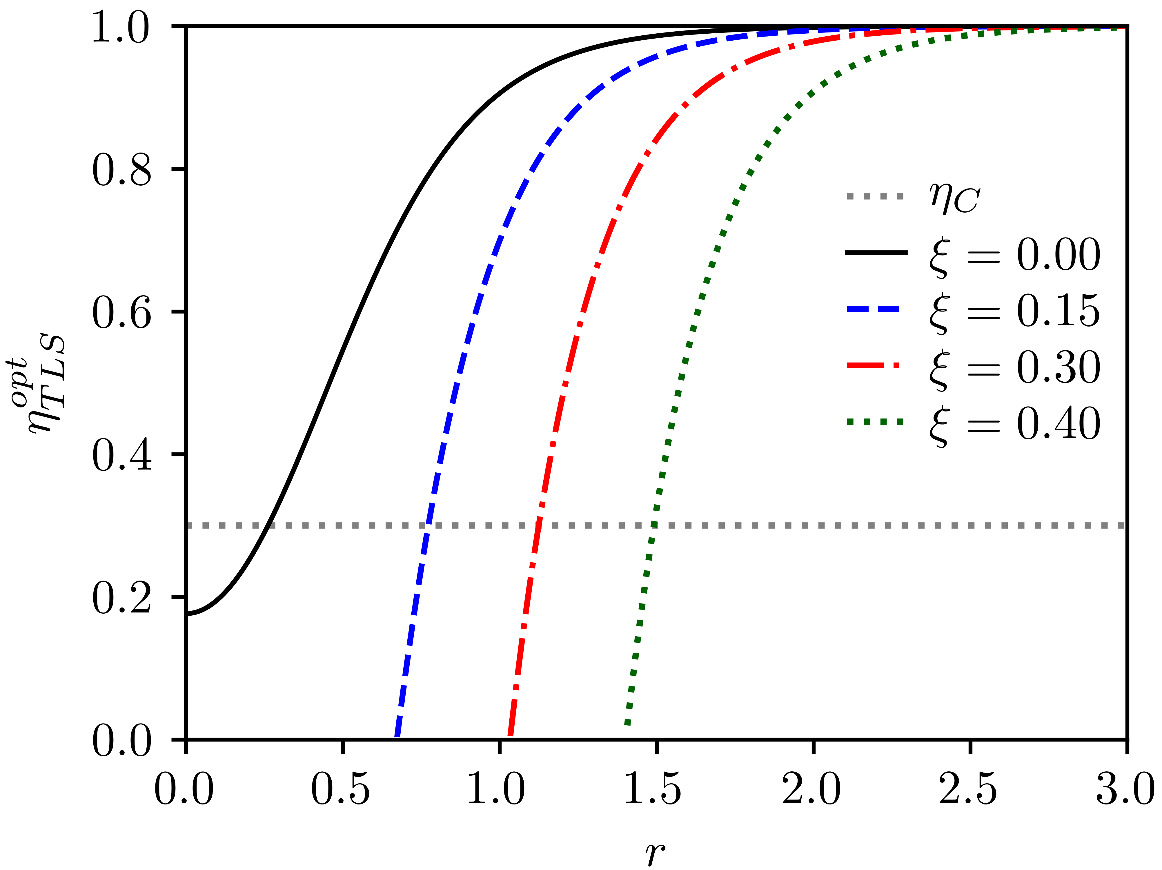
So far, non-null power scenario was not fully explored when using squeezed reservoirs. Thus, for the first time, we show how Carnot efficiency can be surpassed even far from the quasi-static regime with our TLS model. For this purpose, consider a specific case of our engine, the case where $\beta_{h}/\beta_{c}=0.7$, to visualize the behavior of $\eta_{LTS}^{opt}$ (Eq. (5)) by varying both the squeezing $r$ and adiabaticity $\xi$ parameters. For this case, Fig. 1 shows the values of $r$ and $\xi$ in which the net work is extracted from the engine: in the white region there is no extraction of work, since Eq. (4) is not satisfied. The blue region indicates enhancement in the QOHE as compared to the conventional Carnot engine, which is maximum at the quasi-static regime. The narrow red region indicates where the Carnot efficiency is not surpassed. Note that, even in the finite-time regime ($\xi>0$) the efficiency can surpass the Carnot efficiency. Besides, in Fig. 2 we show the efficiency $\eta_{TLS}^{opt}$ versus the squeezing parameter $r$ for several values of the adiabaticity parameter $\xi$. The optimized efficiencies are shown for $\xi=0$ (solid black line), $\xi=0.15$ (dashed blue line), $\xi=0.3$ (dash-dotted red line), and $\xi=0.4$ (dotted green line). The Carnot efficiency $\eta_{C}$ is indicated by the horizontal dotted gray line. We can see in Fig. 2 that $\eta_{LTS}^{opt}$ can overcome $\eta_{C}$ and tends the unity to several different values of $\xi$. The important point to be noted here is that we can now execute the expansion and compression strokes quickly and still obtain high efficiencies, thus bypassing the inconvenient internal friction (dissipation of useful energy) that occurs with the decrease in $\tau$ Plastina et al. 2014; Cakmak et al. 2016; Peterson et al. 2019.

Now we compare our result with that obtained in Ref. Roßnagel et al. 2014. In that work, the authors address only the quasi-static regime of a QOHE based on a HO operating with a squeezed thermal reservoir. The optimized efficiency obtained by them (Eq. (6) of Ref. Roßnagel et al. 2014, takes the form

To our TLS model, replacing $\xi=0$ in Eq. (7), we have

To better appreciate the differences between the TLS and that of the HO models, in Fig. 3 we show both the optimized efficiencies $\eta_{TLS}^{opt}$ (solid blue line) and $\eta_{HO}^{opt}$ (dashed red line) versus the squeezing parameter $r$ for the ratio $\beta_{h}/\beta_{c}=0.7$. We can see that, for the same value of the squeezing parameter, our model provides a larger efficiency. This is a significant enhancement in the efficiency as compared with Ref. Roßnagel et al. 2014.

Next, aiming implementation in NMR Peterson et al. 2019; de Assis et al. 2019, we adopt the following parameters: $\omega_{c}=2\pi\times 2.5$ kHz, $\omega_{h}=10\omega_{c}$, $\beta_{c}=1/\left(10\ \text{peV}\right)$ , and $\beta_{h}=0.7\beta_{c}$. Since these parameters result in $\theta_{c}\approx 0.52$ and $\theta_{h}\approx 3.62$, which means that condition $\theta_{c\left(h\right)}\ll 1$ is not satisfied, it will be necessary to abandon Eq. (7) and extract numerical information directly from Eq. (5). In the context of NMR, the time evolution operator to be considered is $U={\cal T}\text{e}^{-\left(i/\hbar\right)\int_{0}^{\tau}H\left(t\right)dt}$, with ${\cal T}$ being the time ordering operator and $H\left(t\right)=\frac{1}{2}\hbar\left[\omega_{c}\left(1-\frac{t}{\tau}\right)+\omega_{h}\frac{t}{\tau}\right]\left[\cos\left(\frac{\pi t}{2\tau}\right)\sigma_{x}+\sin\left(\frac{\pi t}{2\tau}\right)\sigma_{y}\right]$. Fig. 4 shows the graph of the adiabaticity parameter $\xi$ as a function of time $\tau$ for the given time evolution operator. In Fig. 5 we show the efficiency $\eta_{TLS}$ as a function of the squeezing parameter $r$ for the adiabatic parameters $\xi=0$ (solid black line), $\xi=0.1$ (dashed blue line), $\xi=0.2$ (dotted red line), and $\xi=0.3$ (dash-dotted green line). For comparison, Fig. 5 also shows the Carnot efficiency $\eta_{C}=1-\beta_{h}/\beta_{c}$ (dotted gray line). As we can see, the experimental parameters available, although impose limit to the efficiency attained, allow to obtain efficiencies surpassing Carnot efficiency even for processes occurring far from quasi-static regime.

We have proposed a quantum Otto heat engine based on a two-level system as the working substance that operates under two reservoirs: a cold thermal reservoir and a squeezed hot thermal reservoir. While for typical scenarios Carnot efficiency is the higher limit and can be achieved only for quasi-static processes, in this work we have demonstrated that it is possible to surpass Carnot efficiency even in the finite-time regime (at non null power). Also, we showed that given the same squeezing parameter and the same temperature ratios, the two-level system model exhibits higher efficiency at maximum power as compared to the harmonic oscillator model.

We acknowledge financial support from the Brazilian agencies, CAPES (Financial code 001) CNPq and FAPEG. This work was performed as part of the Brazilian National Institute of Science and Technology (INCT) for Quantum Information Grant No. 465469/2014-0.

References

- Kieu (2004) T. D. Kieu, Phys. Rev. Lett. 93, 140403 (2004).
- Quan et al. (2007) H. T. Quan, Y.-x. Liu, C. P. Sun, and F. Nori, Phys. Rev. E 76, 031105 (2007).
- Wang et al. (2009) H. Wang, S. Liu, and J. He, Phys. Rev. E 79, 041113 (2009).
- Linden et al. (2010) N. Linden, S. Popescu, and P. Skrzypczyk, Phys. Rev. Lett. 105, 130401 (2010).
- Scully et al. (2011) M. O. Scully, K. R. Chapin, K. E. Dorfman, M. B. Kim, and A. Svidzinsky, Proceedings of the National Academy of Sciences 108, 15097 (2011), https://www.pnas.org/content/108/37/15097.full.pdf .
- Wang et al. (2012) J. Wang, Z. Wu, and J. He, Phys. Rev. E 85, 041148 (2012).
- Rahav et al. (2012) S. Rahav, U. Harbola, and S. Mukamel, Phys. Rev. A 86, 043843 (2012).
- Gelbwaser-Klimovsky et al. (2013) D. Gelbwaser-Klimovsky, R. Alicki, and G. Kurizki, Phys. Rev. E 87, 012140 (2013).
- Uzdin et al. (2015) R. Uzdin, A. Levy, and R. Kosloff, Phys. Rev. X 5, 031044 (2015).
- Kosloff and Rezek (2017) R. Kosloff and Y. Rezek, Entropy 19, 136 (2017).
- Huang et al. (2017) X. L. Huang, Y. F. Shang, D. Y. Guo, Q. Yu, and Q. Sun, Quantum Information Processing 16, 174 (2017).
- Zhao and Zhang (2017) L.-M. Zhao and G.-F. Zhang, Quantum Information Processing 16, 216 (2017).
- Brandner et al. (2017) K. Brandner, M. Bauer, and U. Seifert, Phys. Rev. Lett. 119, 170602 (2017).
- Niedenzu et al. (2018) W. Niedenzu, V. Mukherjee, A. Ghosh, A. G. Kofman, and G. Kurizki, Nature Communications 9, 165 (2018).
- Dorfman et al. (2018) K. E. Dorfman, D. Xu, and J. Cao, Phys. Rev. E 97, 042120 (2018).
- Camati et al. (2019) P. A. Camati, J. F. G. Santos, and R. M. Serra, Phys. Rev. A 99, 062103 (2019).
- Türkpençe and Altintas (2019) D. Türkpençe and F. Altintas, Quantum Information Processing 18, 255 (2019).
- Peterson et al. (2019) J. P. S. Peterson, T. B. Batalhão, M. Herrera, A. M. Souza, R. S. Sarthour, I. S. Oliveira, and R. M. Serra, Phys. Rev. Lett. 123, 240601 (2019).
- Bera et al. (2019) M. N. Bera, A. Riera, M. Lewenstein, Z. B. Khanian, and A. Winter, Quantum 3, 121 (2019).
- Çakmak and Altintas (2020) S. Çakmak and F. Altintas, Quantum Information Processing 19, 248 (2020).
- Roßnagel et al. (2014) J. Roßnagel, O. Abah, F. Schmidt-Kaler, K. Singer, and E. Lutz, Phys. Rev. Lett. 112, 030602 (2014).
- Manzano et al. (2016) G. Manzano, F. Galve, R. Zambrini, and J. M. R. Parrondo, Phys. Rev. E 93, 052120 (2016).
- Klaers et al. (2017) J. Klaers, S. Faelt, A. Imamoglu, and E. Togan, Phys. Rev. X 7, 031044 (2017).
- de Assis et al. (2019) R. J. de Assis, T. M. de Mendonça, C. J. Villas-Boas, A. M. de Souza, R. S. Sarthour, I. S. Oliveira, and N. G. de Almeida, Phys. Rev. Lett. 122, 240602 (2019).
- Scully et al. (2003) M. O. Scully, M. S. Zubairy, G. S. Agarwal, and H. Walther, Science 299, 862 (2003), https://science.sciencemag.org/content/299/5608/862.full.pdf .
- Guéry-Odelin et al. (2019) D. Guéry-Odelin, A. Ruschhaupt, A. Kiely, E. Torrontegui, S. Martínez-Garaot, and J. G. Muga, Rev. Mod. Phys. 91, 045001 (2019).
- Beau et al. (2016) M. Beau, J. Jaramillo, and A. Del Campo, Entropy 18 (2016), 10.3390/e18050168.
- Xiao and Li (2018) B. Xiao and R. Li, Physics Letters A 382, 3051 (2018).
- Wang et al. (2019) J. Wang, J. He, and Y. Ma, Phys. Rev. E 100, 052126 (2019).
- Singh and glu (2020) V. Singh and O. E. M. glu, “Performance bounds of non-adiabatic quantum harmonic otto engine and refrigerator under a squeezed thermal reservoir,” (2020), arXiv:2006.08311 .
- Srikanth and Banerjee (2008) R. Srikanth and S. Banerjee, Phys. Rev. A 77, 012318 (2008).
- Alicki (1979) R. Alicki, Journal of Physics A: Mathematical and General 12, L103 (1979).
- Kosloff (1984) R. Kosloff, The Journal of Chemical Physics 80, 1625 (1984), https://doi.org/10.1063/1.446862 .
- Plastina et al. (2014) F. Plastina, A. Alecce, T. J. G. Apollaro, G. Falcone, G. Francica, F. Galve, N. Lo Gullo, and R. Zambrini, Phys. Rev. Lett. 113, 260601 (2014).
- Cakmak et al. (2016) S. Cakmak, F. Altintas, and O. E. Mustecaplioglu, (2016), 10.1140/epjd/e2017-70443-1, arXiv:1605.02522 .