ABSTRACT: Sterile neutrinos are one of the leading dark matter candidates. Their masses may originate from a vacuum expectation value of a scalar field. If the sterile neutrino couplings are very small and their direct coupling to the inflaton is forbidden by the lepton number symmetry, the leading dark matter production mechanism is the freeze–in scenario. We study this possibility in the neutrino mass range up to 1 GeV, taking into account relativistic production rates based on the Bose–Einstein statistics, thermal masses and phase transition effects. The specifics of the production mechanism and the dominant mode depend on the relation between the scalar and sterile neutrino masses as well as on whether or not the scalar is thermalized. We find that the observed dark matter abundance can be produced in all of the cases considered. We also revisit the freeze–in production of a Higgs portal scalar, pointing out the importance of a fusion mode, as well as the thermalization constraints.

1 Introduction

One of the outstanding mysteries of the Universe is the nature of dark matter (DM). An attractive minimal option is provided by sterile neutrinos, whose existence is strongly suggested by the observed neutrino masses. The smallness of the latter can elegantly be explained by the seesaw mechanism [1, 2, 3, 4, 5, 6]. When the active–sterile neutrino mixing is sufficiently small, the lightest sterile neutrino can be very long–lived and play the role of DM. In the simplest scenario proposed by Dodelson and Widrow [7], such neutrinos can be produced via mixing with the active neutrinos in a thermal bath of the Standard Model (SM) particles, although the sterile neutrinos do not thermalize themselves. This minimal option now appears to be in conflict with a number of observations [8, 9, 10, 11, 12, 13, 14, 15, 16, 17] (see e.g. [18] for a review).

Other production mechanisms have been explored in the literature. Primordial lepton asymmetry could generate the active–sterile transitions via the Shi and Fuller mechanism [19, 20]. This option has been studied extensively in the context of the neutrino Minimal Standard Model ( $\nu$ MSM) [21, 22, 23, 24, 25]. Alternatively, the relic population of sterile neutrinos may be generated via decay of a heavier particle like the inflaton [26, 27], the radion [28] or a general scalar singlet [29, 30, 31, 32, 33, 34]. Other possibilities include sterile neutrino production through pion decays [35], heavy pseudo-Dirac neutrinos [36], interactions of light vector bosons [37, 38], via an axion–like field [39] and parametric resonance [40].

An interesting possibility, which we explore in detail, is to generate the observed relic abundance of the sterile neutrino DM through the freeze–in mechanism [41, 42]. This scenario requires a tiny coupling and a negligible initial DM abundance. The correct relic density is then gradually built up via this feeble coupling along the evolution of the Universe. A successful realization of this mechanism involves an extra scalar field, whose decay produces sterile neutrinos [29, 30]. The vacuum expectation value (VEV) of such a field can be responsible for the Majorana neutrino masses [43, 44]. For a small enough coupling, the freeze–in mechanism is at work and the correct DM density can be produced.

In our work, we perform an in–depth analysis of the freeze–in production of sterile neutrinos in the mass range up to 1 GeV, taking into account different possible production regimes, relativistic reaction rates with the Bose–Einstein distribution function, thermal masses and main effects of the phase transitions. Previous studies have mainly focused on the keV mass range [29, 30, 45, 34, 46], in which case the active–sterile mixing angle is required to be below $10^{-5}$ or so. In our case, the requisite mixing must be much smaller calling for a symmetry justification. The required symmetry can be identified with the neutrino parity which acts on the lightest sterile neutrino only.

We find that the neutrino production often takes place in the relativistic regime, in which case the Bose–Einstein distribution should be used for the initial state scalars. This differs from many previous studies which have resorted to the non–relativistic Maxwell-Boltzmann approximation. In order to take quantum statistics into account, we follow the approach of [47],[48] and extend it to asymmetric reactions. The resulting rate enhancement depends strongly on the thermal masses and ranges from ${\cal O}(1)$ to two orders of magnitude in the vicinity of the 2d order phase transition.

We also take into account the most important effects of the phase transitions. First of all, these affect the presence or absence of certain couplings which depend on scalar VEVs. In addition, the mass change at the phase transition can facilitate particle production.

The DM production modes depend on whether or not the scalar is thermalized. It couples to the SM via the Higgs portal [49, 50, 51]. Then, its thermalization depends on the Higgs portal coupling and the maximal temperature. To this end, we revisit the scalar production through the Higgs portal couplings and the consequent thermalization constraints. We find, in particular, that the $2\rightarrow 1$ reaction (fusion) plays an important role in this analysis.

In this work, we are mainly interested in reproducing the correct DM relic abundance. To this end, we solve the Boltzmann equation for the number density rather than the momentum distribution function (unlike e.g. [34]). We reserve the latter for future work.

The paper is organized as follows. In Section 2, we introduce our model, discuss the leading thermal corrections and compile the current constraints on sterile neutrino DM. In Section 3, we generalize the relativistic reaction rates of [47],[48] to asymmetric reactions. Thermalization constraints are discussed in Section 4. Our main results are presented in Sections 5 and 6. We conclude in Section 7.

2 The model

In this work, we focus on a simple set–up: the SM is extended by a $real$ singlet $S$ and some number of right–handed (sterile) neutrinos $\nu_{R_{i}}$ .⁵⁵ 5 Their number can be significantly larger than 3 as motivated by string theory [52]. Here, a sterile neutrino is defined as a fermion that has a Yukawa coupling with the SM neutrinos as well as a Majorana mass term. The lightest of them is assumed to constitute long–lived dark matter.

We assume that the Majorana masses are produced entirely by the singlet scalar VEV. This can be implemented through a lepton–number discrete symmetry forbidding the bare mass:

S\rightarrow-S~~,~~\nu_{i}\rightarrow i\nu_{i}\;.

(1)

The relevant Lagrangian terms are then

-\Delta{\cal L}={1\over 4}\lambda_{s}S^{4}+{1\over 2}\mu_{s}^{2}S^{2}+{1\over 2}\lambda_{hs}|H|^{2}S^{2}+{1\over 2}\lambda_{ij}S\;\nu_{R_{i}}\nu_{R_{j}}+y_{ij}H^{c}\;\bar{l}_{i}\nu_{R_{j}}\;.

(2)

The above symmetry results in 2 useful properties:

•

no inflaton coupling to $\nu_{R_{i}}\nu_{R_{j}}$ is allowed (assuming that the inflaton carries no lepton charge). Otherwise, inflaton decay would normally dominate the neutrino production.
•

diagonalizing the neutrino mass matrix diagonalizes the $S$ coupling to neutrinos (neglecting the Dirac contributions). As a result, there is no flavor change and a heavier $\nu$ cannot produce a lighter $\nu$ via its decay with $S$ –emission. Thus, we can focus on direct freeze–in production of the lightest $\nu$ .

Let us denote the lightest mostly–sterile neutrino $\nu$ and its coupling to $S$ $\lambda$ :

-\Delta{\cal L}={1\over 2}\lambda\;S\;\nu\nu\;.

(3)

Its mass is then $M=\lambda\langle S\rangle$ neglecting the Dirac mass contribution. Throughout this paper we assume that the relevant Yukawa couplings are very small such that the usual Higgs decay does not produce a significant amount of dark matter. The resulting active–sterile mixing angle $\Theta\sim y\langle H\rangle/\lambda\langle S\rangle\ll 10^{-5}$ is also very small.

2.1 The scalar sector

The scalar sector of the model includes the Higgs field $H$ and the real scalar $S$ . The potential invariant under the $S\rightarrow-S$ symmetry is given by

\displaystyle V(h,s)=\frac{\lambda_{h}}{4}h^{4}+\frac{\lambda_{hs}}{4}h^{2}S^{2}+\frac{\lambda_{s}}{4}S^{4}+\frac{1}{2}\;\mu_{h}^{2}\,h^{2}+\frac{1}{2}\mu_{s}^{2}\,S^{2}\,.

(4)

Here we use the unitary gauge $H=(0,h/\sqrt{2})^{T}$ . Both $H$ and $S$ must develop non–zero VEVs $v$ and $u$ , respectively. These are given by


$\displaystyle v^{2}$	$\displaystyle=\frac{2\lambda_{hs}\mu_{s}^{2}-4\lambda_{s}\mu_{h}^{2}}{4\lambda_{h}\lambda_{s}-\lambda_{hs}^{2}}$	(5a)
$\displaystyle u^{2}$	$\displaystyle=\frac{2\lambda_{hs}\mu_{h}^{2}-4\lambda_{h}\mu_{s}^{2}}{4\lambda_{h}\lambda_{s}-\lambda_{hs}^{2}}\;.$	(5b)

The mass matrix at this point is

\displaystyle{\cal M}^{2}=\left(\begin{array}[]{cc}2\lambda_{h}v^{2}&\lambda_{hs}vu\\ \lambda_{hs}vu&2\lambda_{s}u^{2}\end{array}\right)\,.

Since the couplings are real and we require $v^{2}>0,u^{2}>0$ , the mass matrix ${\cal M}^{2}$ is positive definite if and only if

\lambda_{h}>{\lambda_{hs}^{2}\over 4\lambda_{s}}~~,~~\lambda_{s}>0~.

(8)

${\cal M}^{2}$ can be diagonalized by the orthogonal transformation

\displaystyle O^{T}{\cal M}^{2}O=\textrm{diag}(m_{1}^{2},m_{2}^{2})~,

(9)

where

\displaystyle O

\displaystyle=\left(\begin{array}[]{cc}\cos\theta&\sin\theta\\ -\sin\theta&\cos\theta\end{array}\right)\;

and the angle $\theta$ satisfies

\displaystyle\tan 2\theta

\displaystyle=\frac{\lambda_{hs}vu}{\lambda_{s}u^{2}-\lambda_{h}v^{2}}\,.

(12)

The mass squared eigenvalues are given by

\displaystyle m_{1,2}^{2}=\lambda_{h}v^{2}+\lambda_{s}u^{2}\mp\frac{\lambda_{s}u^{2}-\lambda_{h}v^{2}}{\cos 2\theta}\,.

(13)

The above equation implies $\textrm{sign}(m_{2}^{2}-m_{1}^{2})=\textrm{sign}(\cos 2\theta)\,\textrm{sign}(\lambda_{s}u^{2}-\lambda_{h}v^{2})$ . We will primarily be interested in the small mixing case. (E.g., for a light singlet, the meson decay and LEP constraints on the mixing angle are very strong [53].) Thus, it is convenient to employ the small angle approximation $\sin\theta\ll 1$ and neglect the $\theta^{2}$ –terms. In this case, the eigenvalues can be relabelled according to the state composition and satisfy

m_{h}^{2}\simeq 2\lambda_{h}v^{2}~~,~~m_{s}^{2}\simeq 2\lambda_{s}u^{2}\;.

(14)

The mixing angle can then be expressed as

\theta\simeq{\lambda_{hs}\over\sqrt{4\lambda_{h}\lambda_{s}}}~{m_{s}m_{h}\over m_{s}^{2}-m_{h}^{2}}\;.

(15)

This form is convenient since stability considerations bound the first factor by 1. Clearly, for $m_{s}$ close to $m_{h}$ our approximation fails. When $m_{h}$ and $m_{s}$ are substantially different, the mixing angle is bounded by $|\theta|<m_{s}/m_{h}\;,m_{h}/m_{s}$ . In most of our parameter space, the mixing angle is indeed very small.

In what follows, the sign of $\theta$ is unimportant, so will denote by $\theta$ the magnitude of the mixing angle.

2.1.1 Thermal corrections

At high temperature, the scalar potential gets modified by the thermal corrections. The main effect is captured by the thermal masses which amount to the replacements

\mu_{h}^{2}\rightarrow\mu_{h}^{2}+c_{h}T^{2}~~,~~\mu_{s}^{2}\rightarrow\mu_{s}^{2}+c_{s}T^{2}\;,

(16)

where

	$\displaystyle c_{h}\simeq{3\over 16}g^{2}+{1\over 16}g^{\prime 2}+{1\over 4}y_{t}^{2}+{1\over 2}\lambda_{h}\;,$
	$\displaystyle c_{s}={1\over 4}\lambda_{s}+{1\over 6}\lambda_{hs}\;.$		(17)

Here $g,g^{\prime}$ are the SM gauge couplings and $y_{t}$ is the top–quark Yukawa coupling. At high $T$ , the minimum of the potential is at $v=u=0$ . The transition to non-zero VEVs takes place at the critical temperatures: $v=0\rightarrow v\not=0$ at $T_{c}^{v}$ and $u=0\rightarrow u\not=0$ at $T_{c}^{u}$ . The dynamics of the transition is somewhat complicated and proceeds in steps: at the first stage, one of the VEVs stays zero and the other becomes non–zero, while at the second stage both of the fields attain non–zero VEVs. On the other hand, we find that the neutrino DM production depends on the critical temperature rather weakly. Therefore, it suffices for our purposes to approximate the critical temperature by that of the first stage, $T_{c}^{2}=|\mu_{i}^{2}|/c_{i}$ . The critical temperatures can then be expressed in terms of the physical masses and the couplings for $\sin\theta\ll 1$ :

	$\displaystyle T_{c}^{v}={\|\mu_{h}\|\over\sqrt{c_{h}}}\;,$
	$\displaystyle T_{c}^{u}={\|\mu_{s}\|\over\sqrt{c_{s}}}\;,$
	$\displaystyle-\mu_{h}^{2}={\lambda_{hs}\over 4\lambda_{s}}\;m_{s}^{2}+{1\over 2}m_{h}^{2}\;,$
	$\displaystyle-\mu_{s}^{2}={\lambda_{hs}\over 4\lambda_{h}}\;m_{h}^{2}+{1\over 2}m_{s}^{2}\;.$		(18)

It is important to include the thermal masses (16) in the calculation of the reaction rates. This is dictated by their correct high temperature behaviour.

The neutrino thermal masses, on the other hand, can be neglected since these are suppressed by $\lambda^{2}$ .

2.2 Constraints on sterile neutrino dark matter

In Fig. 1, we collect the most stringent limits on the active–sterile mixing $\sin^{2}\Theta$ as a function of the sterile neutrino mass $M$ . We assume the abundance of sterile neutrinos to be equal to the dark matter density measured by Planck [54, 55]. Since our dark matter candidate decays into active neutrinos and other SM states, there are various strong constraints on this scenario. The most relevant $\nu$ decay modes are [56, 57, 58, 18]:

$\displaystyle\Gamma_{\nu_{a}\gamma}$	$\displaystyle=$	$\displaystyle\frac{9\alpha_{EM}G_{f}^{2}M^{5}}{256\pi^{4}}\rm sin^{2}\Theta\,,$	(19)
$\displaystyle\Gamma_{\nu_{a}e^{+}e^{-}}$	$\displaystyle=$	$\displaystyle\theta(M-2m_{e})\frac{G_{f}^{2}M^{5}}{96\pi^{3}}\rm sin^{2}\Theta\frac{(1+4sin^{2}\theta_{w}+8sin^{4}\theta_{w})}{4}\,,$
$\displaystyle\Gamma_{\nu_{a}\pi^{0}}$	$\displaystyle=$	$\displaystyle\theta(M-m_{\pi^{0}})\frac{G_{f}^{2}M^{3}f_{\pi^{0}}^{2}}{32\pi}\rm sin^{2}\Theta\left(1-{m_{\pi^{0}}^{2}\over M^{2}}\right)^{2}\,,$
$\displaystyle\Gamma_{\nu_{a}\nu_{a}\bar{\nu}_{a}}$	$\displaystyle=$	$\displaystyle\frac{G_{f}^{2}M^{5}}{96\pi^{3}}\rm sin^{2}\Theta\,,$

where $\nu_{a}$ indicates an active neutrino. For a heavier $\nu$ , further decay modes become relevant, e.g. those involving muons. Here we are assuming that the mixing with the electron neutrino dominates.

In the dark grey region, the sterile neutrino lifetime is shorter than the age of the Universe. Sterile neutrinos are always produced in a thermal bath via the sterile–active mixing. This leads to the “overproduction” constraint indicated by the dashed purple line, above which the sterile neutrino abundance exceeds that of dark matter.

Refer to caption — Figure 1: Neutrino dark matter constraints on the active–sterile mixing angle $\Theta$ . The shaded areas are excluded by: X-ray data (dark blue), NuSTAR (dark cyan), Fermi-GBM (red), INTEGRAL (green), COMPTEL (magenta), EGRET (orange), Fermi-LAT (red). In the dark grey region, the sterile neutrino lifetime is shorter than the age of the Universe. Above the purple dashed line the sterile neutrino is overabundant (assuming production only via mixing with active neutrinos). The CMB constraints are given by the yellow dashed lines.

The sterile neutrino radiative decay is particularly relevant for X-ray and gamma-ray line searches. For sterile neutrino masses $M\lesssim 50$ keV, searches of decaying dark matter signals have been carried out using a wide range of X-ray telescopes like XMM-Newton [8, 59], Suzaku [60], HEAO-1 [8], INTEGRAL [14, 13], Swift [61] and CHANDRA [62, 63]. We collect most of them in the dark blue shaded area.⁶⁶ 6 This bound takes into account the uncertainty in the dark matter density, as in [64]. Among them, the CHANDRA satellite provides the strongest limits [17]. Most recent bounds from the X-ray microcalorimeter NuSTAR [65], looking at the Galactic Bulge, are displayed in dark cyan. The limits from searches for sterile neutrino decay lines using the Gamma-ray Burst Monitor onboard the Fermi Gamma-Ray Space Telescope (Fermi-GBM) [66] are shown in red. The green region is further constrained by INTEGRAL [13] searching for spectral lines from dark matter with a mass up to 14 MeV, decaying in the Milky Way halo. Gamma-ray lines searches further constrain our sterile neutrino dark matter parameter space at higher masses: we show the bounds from COMPTEL [67, 58] (magenta), EGRET [68, 58] (orange) and Fermi Large Area Telescope (Fermi-LAT) [16] (red).

Finally, measurements of the cosmic microwave background (CMB) allow us to constrain sterile neutrino decays leading to early energy injections [69, 70, 71, 72, 73]. The relevant decay modes are $\nu_{a}e^{+}e^{-}$ and to $\nu_{a}\gamma$ . Using the bounds on the corresponding decay rates from Ref. [74] with appropriate photon flux rescaling, we obtain the CMB bounds shown by the yellow dashed lines.

We see that the resulting constraints on the mixing angle are very strong. For example, for $M$ close to 1 GeV, the bound on $\Theta$ is of order $10^{-18}$ . Such small values appear unnatural. Within our simple model, the angles are input parameters, while in various extensions their small values can be justified by flavor–dependent symmetry. Indeed, in addition to the lepton number $Z_{4}$ , one may impose a $Z_{2}$ symmetry which acts on the lightest Majorana neutrino $\nu_{R_{1}}$ :

\nu_{R_{1}}\rightarrow-\nu_{R_{1}}~~\Rightarrow~~\Theta=0\;.

(20)

This forbids the corresponding Yukawa couplings and sets $\Theta=0$ . Assuming that this $Z_{2}$ is broken at some scale, the effective Yukawa couplings can be generated by higher dimensional operators. As a result, very small mixing angles can be generated. Since in the limit $\Theta\rightarrow 0$ the system becomes more symmetric, small mixing angles are natural according to the t’Hooft criterion [75].

Since the lightest sterile neutrino effectively decouples from the Standard Model, the active neutrino masses are generated by the heavier $\nu_{R_{i}}$ . The usual seesaw result for the active neutrino mass matrix $M_{\nu}$ still applies: $M_{\nu}=(M_{D})^{T}M^{-1}M_{D}$ , where $M_{D}$ is the Dirac mass matrix and $M$ is the diagonal Majorana mass matrix. Since we leave the total number of sterile neutrinos arbitrary, no relevant, model independent, constraints are imposed by the low energy neutrino data [21].

Longevity of the lightest sterile neutrino can be achieved at small masses and/or small mixings. While most research efforts have focused on the first option, here we are considering the second possibility in more detail. We also see that, given the vast $(\Theta,M)$ parameter space, dark matter decay may be observed, e.g. via monochromatic X- or gamma rays.

3 Relativistic rates for asymmetric reactions

Neutrino dark matter can be produced through a number of reactions. These include both scattering and decay which take place in the relativistic regime, i.e. when the temperature exceeds the particle masses. Since there are bosons in the initial state, relativistic Bose–Einstein enhancement can be very significant and the reaction rates must take it into account. The relevant results for symmetric reactions, that is, involving particles with the same mass in the initial state, have been obtained in [47],[48]. In our case, some reactions can be asymmetric, e.g. $H+S\rightarrow X$ , and these results must be generalized to particles of different masses.

In this section, we generalize the relativistic reaction rates based on the Bose–Einstein statistics [47],[48] to processes involving particles with different masses. The $a\rightarrow b$ reaction rate per unit volume is given by the general expression

\Gamma_{a\rightarrow b}=\int\left(\prod_{i\in a}{d^{3}{\bf p}_{i}\over(2\pi)^{3}2E_{i}}f(p_{i})\right)~\left(\prod_{j\in b}{d^{3}{\bf p}_{j}\over(2\pi)^{3}2E_{j}}(1+f(p_{j}))\right)|{\cal M}_{a\rightarrow b}|^{2}~(2\pi)^{4}\delta^{4}(p_{a}-p_{b}).

(21)

Here ${\cal M}_{a\rightarrow b}$ is the QFT transition amplitude, in which we also absorb the initial and final state symmetry factors, and $f(p)$ is the momentum distribution function. For the freeze–in scenario, the density of the final state particles is small so that the enhancement factors $1+f(p_{j})$ can be set to one. On the other hand, it is important to keep the full Bose–Einstein distribution functions $f(p_{i})$ for the initial state and their replacement by the Maxwell–Boltzmann ones can lead to a rate underestimate by orders of magnitude.

We are particularly interested in the $2\rightarrow 2$ reactions. The reaction rate can be expressed in terms of the cross-section,

\Gamma_{22}=(2\pi)^{-6}\int d^{3}{\bf p_{1}}d^{3}{\bf p_{2}}~f(p_{1})f(p_{2})~\sigma(p_{1},p_{2})v_{\rm M\o l}

(22)

with

v_{\rm M\o l}={F\over E_{1}E_{2}}\equiv{\sqrt{(p_{1}\cdot p_{2})^{2}-m_{1}^{2}m_{2}^{2}}\over E_{1}E_{2}}\;,

(23)

f(p)={1\over\exp^{u\cdot p\over T}-1}~~,~~u=(1,0,0,0)^{T}\;.

(24)

The cross section is defined by

\sigma(p_{1},p_{2})={1\over 4F(p_{1},p_{2})}\int|{\cal M}|^{2}(2\pi)^{4}\delta^{4}\left(p_{1}+p_{2}-\sum_{i}k_{i}\right)\prod_{i}{d^{3}{\bf k}_{i}\over(2\pi)^{3}2E_{k_{i}}}\;,

(25)

where ${\cal M}$ is the QFT transition amplitude. Here we absorb the symmetry factors for the initial state directly into $\sigma(p_{1},p_{2})$ .

The calculation is most easily performed in the center–of–mass (CM) frame, so let us convert the integral into that frame. The CM frame for each pair $p_{1},p_{2}$ is the frame where $p_{1}+p_{2}$ has only zero spacial components. Let us consider how the integration measure transforms as we go to the CM frame. The Lorentz invariant measure is

{d^{3}{\bf p_{1}}\over 2E_{1}}{d^{3}{\bf p_{2}}\over 2E_{2}}=d^{4}p_{1}d^{4}p_{2}~\delta(p_{1}^{2}-m_{1}^{2})\delta(p_{2}^{2}-m_{2}^{2})\;.

(26)

Introduce

p={p_{1}+p_{2}\over 2}~,~k={p_{1}-p_{2}\over 2}~,

(27)

such that

d^{4}p_{1}d^{4}p_{2}~\delta(p_{1}^{2}-m_{1}^{2})\delta(p_{2}^{2}-m_{2}^{2})=2^{4}d^{4}p~d^{4}k~\delta((p+k)^{2}-m_{1}^{2})\delta((p-k)^{2}-m_{2}^{2})\;.

(28)

Any time-like vector $p$ can be Lorentz-transformed to the form

p=\Lambda(p)~\left(\begin{matrix}&E&\\ &0&\\ &0&\\ &0&\end{matrix}\right),

(29)

with the explicit parametrization in terms of rapidity $\eta$ and angular coordinates $\theta,\phi$ being

	$\displaystyle p^{0}=E\cosh\eta,$
	$\displaystyle p^{1}=E\sinh\eta\sin\theta\sin\phi,$
	$\displaystyle p^{2}=E\sinh\eta\sin\theta\cos\phi,$
	$\displaystyle p^{3}=E\sinh\eta\cos\theta.$

In other words, in the convention $p=(p^{0},p^{3},p^{2},p^{1})^{T}$ , we have

	$\displaystyle\Lambda(p)=\left(\begin{matrix}&1&0&0&0&\\ &0&1&0&0&\\ &0&0&\cos\phi&-\sin\phi&\\ &0&0&\sin\phi&\cos\phi&\end{matrix}\right)\left(\begin{matrix}&1&0&0&0&\\ &0&\cos\theta&-\sin\theta&0&\\ &0&\sin\theta&\cos\theta&0&\\ &0&0&0&1&\end{matrix}\right)\left(\begin{matrix}&\cosh\eta&\sinh\eta&0&0&\\ &\sinh\eta&\cosh\eta&0&0&\\ &0&0&1&0&\\ &0&0&0&1&\end{matrix}\right),$
	$\displaystyle\Lambda(p)^{-1}=\left(\begin{matrix}&\cosh\eta&-\sinh\eta&0&0&\\ &-\sinh\eta&\cosh\eta&0&0&\\ &0&0&1&0&\\ &0&0&0&1&\end{matrix}\right)\left(\begin{matrix}&1&0&0&0&\\ &0&\cos\theta&\sin\theta&0&\\ &0&-\sin\theta&\cos\theta&0&\\ &0&0&0&1&\end{matrix}\right)\left(\begin{matrix}&1&0&0&0&\\ &0&1&0&0&\\ &0&0&\cos\phi&\sin\phi&\\ &0&0&-\sin\phi&\cos\phi&\end{matrix}\right).$

The $p$ -vector in the form $(E,0,0,0)^{T}$ corresponds to the CM frame and $E>0$ is half the CM energy. The $p$ -integration measure becomes

d^{4}p=\sinh^{2}\eta E^{3}dE~d\eta~d\Omega_{p}\;,

(31)

where $\Omega_{p}$ is the solid angle in $p$ -space. Now apply the same Lorentz transformation $\Lambda(p)$ to the vector $k$ ,

	$\displaystyle k=\Lambda(p)~k^{\prime}$	$\displaystyle\xrightarrow{\text{ drop~the~prime}}$	$\displaystyle k,$
	$\displaystyle d^{4}k=d^{4}k^{\prime}$	$\displaystyle\xrightarrow{\text{ drop~the~prime}}$	$\displaystyle d^{4}k\equiv dk_{0}\|{\bf k}\|^{2}d\|{\bf k}\|d\Omega_{k}\;,$		(32)

where we have used the fact that $\Lambda(p)$ is a constant Lorentz transform with respect to the variable $k$ so that the measure remains invariant. We drop the prime for convenience, remembering that $k$ now is in the CM frame. $\Omega_{k}$ denotes the corresponding solid angle in that frame.

Let us now integrate the delta functions. We can explicitly integrate over $k_{0}$ and $|{\bf k}|$ . In the CM frame, the delta functions become

\delta(E^{2}+2Ek_{0}+k_{0}^{2}-{\bf k}^{2}-m_{1}^{2})~\delta(E^{2}-2Ek_{0}+k_{0}^{2}-{\bf k}^{2}-m_{2}^{2})\;.

(33)

This enforces

	$\displaystyle k_{0}={m_{1}^{2}-m_{2}^{2}\over 4E}\;,$
	$\displaystyle{\bf k}^{2}=E^{2}-{m_{1}^{2}+m_{2}^{2}\over 2}+{(m_{1}^{2}-m_{2}^{2})^{2}\over 16E^{2}}\;.$		(34)

We then have

\displaystyle\int dk_{0}d|{\bf k}||{\bf k}|^{2}~\delta(E^{2}+2Ek_{0}+k_{0}^{2}-{\bf k}^{2}-m_{1}^{2})~\delta(E^{2}-2Ek_{0}+k_{0}^{2}-{\bf k}^{2}-m_{2}^{2})={|{\bf k}|\over 8E}\;,

which allows us to rewrite the integration measure as

\int{d^{3}{\bf p_{1}}\over 2E_{1}}{d^{3}{\bf p_{2}}\over 2E_{2}}...={1\over 2}\int_{m_{1}+m_{2}\over 2}^{\infty}dE~E~\sqrt{(4E^{2}-m_{1}^{2}-m_{2}^{2})^{2}-4m_{1}^{2}m_{2}^{2}}\int_{0}^{\infty}d\eta~\sinh^{2}\eta~\int d\Omega_{p}~d\Omega_{k}...\;,

(35)

where in the integrand one must set $k_{0}$ and $|{\bf k}|$ to their values given by Eq. (34). Note that $E$ is half the CM energy.

Since the cross section in the CM frame is a function of $E$ only, the angular dependence comes entirely from the distribution functions. We have

	$\displaystyle u\cdot p_{1}=(\Lambda^{-1}u)\cdot(p+k)=(E+k_{0})\cosh\eta+\|{\bf k}\|\sinh\eta~\cos\theta_{k}\;,$
	$\displaystyle u\cdot p_{2}=(\Lambda^{-1}u)\cdot(p-k)=(E-k_{0})\cosh\eta-\|{\bf k}\|\sinh\eta~\cos\theta_{k}\;.$		(36)

Here we have used $k^{3}=|{\bf k}|\cos\theta_{k}$ .

Integration over $\Omega_{p}$ gives $4\pi$ and the integral over $\phi_{k}$ is $2\pi$ . Let us now integrate over $\theta_{k}$ . The integral can be reduced to

\displaystyle I_{\theta}=\int_{-1}^{1}dx~{1\over e^{a+bx}-1}{1\over e^{c-bx}-1}

\displaystyle=

\displaystyle{1\over b(e^{a+c}-1)}\ln{\left[{\sinh{a+b\over 2}\over\sinh{a-b\over 2}}~{\sinh{c+b\over 2}\over\sinh{c-b\over 2}}\right]}

(37)

for $a,c>b$ . Here $a={(E+k_{0})\cosh\eta\over T}$ , $c={(E-k_{0})\cosh\eta\over T}$ and $b={|{\bf k}|\sinh\eta\over T}$ . (This result can most easily be obtained by the change of variables to $y=e^{bx}$ .)

We thus get

	$\displaystyle\Gamma_{22}=(2\pi)^{-6}\int{d^{3}{\bf p_{1}}\over 2E_{1}}{d^{3}{\bf p_{2}}\over 2E_{2}}~f(p_{1})f(p_{2})~4F(p_{1},p_{2})\;\sigma(p_{1},p_{2})$
	$\displaystyle={T\over 4\pi^{4}}\int_{m_{1}+m_{2}\over 2}^{\infty}dE~E^{2}\int_{0}^{\infty}d\eta{\sinh\eta\over e^{{2E\over T}\cosh\eta}-1}~\ln\left[{\sinh{(E+k_{0})\cosh\eta+\|{\bf k}\|\sinh\eta\over 2T}\over\sinh{(E+k_{0})\cosh\eta-\|{\bf k}\|\sinh\eta\over 2T}}~{\sinh{(E-k_{0})\cosh\eta+\|{\bf k}\|\sinh\eta\over 2T}\over\sinh{(E-k_{0})\cosh\eta-\|{\bf k}\|\sinh\eta\over 2T}}\right]$
	$\displaystyle\times 4F\sigma^{\rm CM}(E)\;,$		(38)

with $k_{0}$ and $|{\bf k}|$ given by (34). This expression reduces to that of [47],[48] for equal masses, $m_{1}=m_{2}$ .

It is important to note that the masses here must include thermal corrections (16). This is necessary for the correct high temperature behaviour:

\Gamma_{22}\propto T^{4}\ln{T\over m}\rightarrow{\rm const}\;T^{4}

(39)

only when a thermal correction to $m$ has been included. The latter also regularizes the infrared divergence in the massless limit.

4 Thermalization constraints

In this work, we focus on freeze–in production of sterile neutrinos. Freeze–in calculations are reliable only if the produced particles do not thermalize. This requires the coupling between the thermal bath and the frozen–in particles as well as self–interaction of the latter to be sufficiently small. In this section, we delineate parameter space consistent with these conditions. We use relativistic formulas for the reaction rates, taking into account quantum statistics for the initial state.

Let us consider the regime where $H$ and $S$ develop VEVs $v$ and $u$ , respectively. We can parametrize them in the unitary gauge as

	$\displaystyle H\rightarrow{1\over\sqrt{2}}(h+v)\;,$
	$\displaystyle S\rightarrow s+u\;.$		(40)

In terms of the 4–component Majorana neutrino $\nu$ , the relevant to our calculation terms in the Lagrangian are

	$\displaystyle-\Delta{\cal L}_{1}$	$\displaystyle=$	$\displaystyle{1\over 2}\lambda\;s\;\bar{\nu}\nu+{1\over 2}M\;\bar{\nu}\nu\;,$		(41)
	$\displaystyle-\Delta{\cal L}_{2}$	$\displaystyle=$	$\displaystyle{1\over 2}m_{h}^{2}h^{2}+{1\over 2}m_{s}^{2}s^{2}+{v\over 2}\lambda_{hs}hs^{2}+{u\over 2}\lambda_{hs}sh^{2}+u\lambda_{s}s^{3}+{1\over 4}\lambda_{hs}h^{2}s^{2}+{1\over 4}\lambda_{s}s^{4}\;,$

where $M=\lambda u$ and we have neglected the scalar mixing. The Majorana notation has the advantage that the $\nu\nu$ final state includes all combinations of 2–component neutrinos and anti–neutrinos.

4.1 Sterile neutrino thermalization

We show in Sec. 5 that the main production channel for sterile neutrinos is the decay $s\rightarrow\nu\nu$ . Here we assume that $s$ is in thermal equilibrium and $m_{s}\gg M$ . For a sufficiently large $\lambda$ , the decay is efficient and the neutrino number density $n_{\nu}(T)$ approaches its equilibrium value at a given temperature, $n_{\nu}^{\rm eq}(T)$ . In this case, the reverse process $\nu\nu\rightarrow s$ becomes important and the neutrinos tend to equilibrate with the thermal bath of $s$ . Thus, we use the non–thermalization criterion

n_{\nu}(T)<n_{\nu}^{\rm eq}(T)

(42)

for any $T$ down to temperatures around $M/3$ . (At lower $T$ , $n_{\nu}^{\rm eq}(T)$ is exponentially suppressed.)

The number density $n_{\nu}$ is calculated via the Boltzmann equation

\dot{n}_{\nu}+3n_{\nu}H=2\Gamma_{12}(s\rightarrow\nu\nu)\;,

(43)

where $H$ is the Hubble rate,

H=\sqrt{\pi^{2}g_{*}\over 90}\;{T^{2}\over M_{\rm Pl}}\;,

(44)

with $g_{*}$ being the number of active SM degrees of freedom. $\Gamma_{12}(s\rightarrow\nu\nu)$ is the reaction rate per unit volume (see Section 5 for an explicit expression). It is calculated with the Bose–Einstein distribution for $s$ , while neglecting the final state Pauli blocking due to the low density of $\nu$ , as is usual in freeze–in computations. Since the issue of bona fide thermalization is quite complicated in any case, this approximation is adequate for our purposes.

Figure 2: Sterile neutrino non–thermalization bound. The neutrinos are produced via

s\rightarrow\nu\nu

with

s

in thermal equilibrium and

m_{s}\gg M

. In the shaded region,

n_{\nu}\gtrsim n_{\nu}^{\rm eq}

such that the reverse process

\nu\nu\rightarrow s

is important.

The solution to the Boltzmann equation for fixed $\lambda,m_{s}$ and zero initial $n_{\nu}$ is then compared to the equilibrium neutrino density at a given $T$ . If inequality (46) is satisfied for any $T$ above $M/3$ , the freeze–in approximation is adequate. Our numerical results for $m_{s}\gg M$ are presented in Fig. 2. In the shaded region, the neutrino density equals or exceeds its equilibrium value. The kink at roughly 1 GeV appears due to the significant change in $g_{*}$ at the QCD phase transition. We see that only quite small couplings, e.g. below $10^{-8}$ at $m_{s}\sim 1$ GeV, are consistent with the freeze–in approximation. The bound can be approximated by

\lambda<5\times 10^{-9}\;\sqrt{m_{s}\over{\rm GeV}}\;.

(45)

The qualitative behaviour of $\lambda(m_{s})$ can be understood from $\lambda^{2}$ -dependence of the rate and the fact that the main contribution to $n_{\nu}$ comes from temperatures of order $m_{s}$ . We discuss this in more detail in Sec. 5.2.

In the vicinity of the shaded region, the neutrino density is significant such that the final state quantum statistics (Pauli blocking) can have a tangible impact on the reaction rate. This effect would reduce the rate, hence our bound is somewhat more restrictive than the true one and can be viewed as conservative.

Let us note that other possible “thermalization” conditions appear in the literature. For example, one can compare the neutrino production rate to the Universe expansion rate. If the former dominates, one expects the neutrino sector to be quickly populated. In our case, this corresponds to $n_{s}^{-1}\Gamma_{12}(s\rightarrow\nu\nu)\gtrsim 3H$ . While such a condition often leads to similar results, there are notable exceptions. In particular, the above inequality is always satisfied at low enough temperatures regardless of the coupling. This, however, does not mean that the neutrino sector gets populated. Indeed, when $s$ is non–relativistic, $n_{s}^{-1}\Gamma_{12}(s\rightarrow\nu\nu)$ is approximately constant, while $H$ decreases as $T^{2}$ . As a result, all the $s$ –quanta available at the corresponding temperature get converted into $\nu$ pairs. Yet, since for relativistic neutrinos $n_{s}^{\rm eq}(T)\ll n_{\nu}^{\rm eq}(T)$ , the neutrino density increase is negligible and $\nu$ ’s do not thermalize. Another exception is the situation in which the production is intense but short in duration, e.g. around a phase transition. In this case, the accumulated density can still be small.

4.2 Thermalization of $s$

In this work, we assume that the dominant source of $s$ –quanta is the Higgs thermal bath. It is important to understand under what circumstances the processes $h\leftrightarrow ss$ , $hh\leftrightarrow ss$ and $hh\leftrightarrow s$ lead to thermalization of $s$ . As in the previous section, we use the criterion

n_{s}(T)<n_{s}^{\rm eq}(T)

(46)

for any $T\raise 1.29167pt\hbox{$\;>$\kern-7.5pt\raise-4.73611pt\hbox{$\sim\;$}}m_{s}$ to ensure non–thermalization of $s$ .⁷⁷ 7 In practice, we check this condition down to temperatures $T\sim m_{s}/3$ , where $s$ becomes non–relativistic. The number density $n_{s}$ is calculated numerically via the Boltzmann equation

\dot{n}_{s}+3n_{s}H=\sum_{i}a_{i}\Gamma_{i}\;,

(47)

where $\Gamma_{i}$ are the reaction rates $\Gamma_{12}(h\rightarrow ss)$ , $\Gamma_{22}(hh\rightarrow ss)$ , $\Gamma_{21}(hh\rightarrow s)$ and $a_{i}$ take into account the number of $s$ –particles in the final state as well as the number of Higgs d.o.f. The explicit expressions for the rates are given in Sec. 6.2.

Figure 3: Upper bounds on

\lambda_{hs}

from non–thermalization of

s

. In the shaded regions,

n_{s}(T)\geq n_{s}^{\rm eq}(T)

due to the

h\rightarrow ss

hh\rightarrow ss

and

hh\rightarrow s

processes. Here the scalar mixing and the electroweak (EW) transition effects have been neglected. The fusion mode

hh\rightarrow s

is sensitive to

\lambda_{s}

, for which two benchmark values

10^{-5}

and

10^{-10}

have been chosen.

The resulting bounds on $\lambda_{hs}$ are shown in Fig. 3. For a light $s$ , the decay mode $h\rightarrow ss$ dominates, while for a heavy scalar the production is typically dominated by the fusion mode $hh\rightarrow s$ . The latter is sensitive to the $s$ –VEV $u=m_{s}/\sqrt{2\lambda_{s}}$ , so additional input such as the coupling $\lambda_{s}$ is required. This VEV grows very large at small $\lambda_{s}$ which results in a large reaction rate. Note that in the vicinity of the shaded region, the final state Bose–Einstein enhancement factor can be non–negligible, so our procedure overestimates somewhat the upper bound on the coupling.

The bound on $\lambda_{hs}$ at $m_{s}\ll m_{h}$ is independent of $m_{s}$ ,

\lambda_{hs}(h\rightarrow ss)<4\times 10^{-8}\;.

(48)

This is because $\Gamma_{12}(h\rightarrow ss)$ is independent of $m_{s}$ in this regime and the production stops around $T\sim m_{h}/5$ . At larger $m_{s}$ , the scattering reaction $hh\rightarrow ss$ becomes significant. The rate $\Gamma_{22}(hh\rightarrow ss)$ scales as $T^{4}$ in the relativistic regime and the resulting $n_{s}(T)\propto T^{2}$ . The yield is dominated by low temperatures consistent with the relativistic scaling, that is, $T\sim m_{s}$ . We thus obtain

\lambda_{hs}(hh\rightarrow ss)<6\times 10^{-8}\;\sqrt{m_{s}\over{\rm GeV}}\;.

(49)

The fusion channel $hh\rightarrow s$ is more complicated. For $m_{s}\gg 2m_{h}$ , it becomes active at temperatures below $T\sim m_{s}$ , that is, when the Higgses still have enough energy to produce $s$ and the Higgs thermal mass is not too large for the process to be kinematically allowed. The fusion becomes inefficient below $T\sim m_{s}/6$ . In this regime, the reaction rate does not follow any simple scaling law and numerically we obtain

\lambda_{hs}(hh\rightarrow s)<6\times 10^{-9}\;\sqrt{\lambda_{s}m_{s}\over{\rm GeV}}\;.

(50)

The appearance of $\lambda_{s}$ can be understood from the reaction rate scaling as $\lambda_{hs}^{2}/\lambda_{s}$ for a fixed $m_{s}$ .

4.2.1 Self–thermalization due to $\lambda_{s}$

Even if $\lambda_{hs}$ is small, the $s$ –sector can thermalize due to self–interaction $\lambda_{s}s^{4}$ . This happens when the number changing processes $ss\leftrightarrow ssss$ become efficient and the density $n_{s}$ starts being sensitive to $\lambda_{s}$ . The specifics of self–thermalization are computationally involved. In the symmetric phase $u=0$ at large $s$ –densities close to equilibrium, the (necessary) thermalization condition on $\lambda_{s}$ has been derived in [47]. Here we are interested in the broken phase $u\not=0$ at low $s$ –densities and thus have to resort to simple estimates. We assume that the initial $n_{s}$ is created via the Higgs thermal bath and study which values of $\lambda_{s}$ do not affect its evolution.

Figure 4: Estimates of the upper bound on

\lambda_{s}

from non–thermalization of

s

. In the shaded regions, the

ss\rightarrow ssss

process is efficient. The bound depends on

n_{s}

and thus is sensitive to

\lambda_{hs}

and the

s

–production mode. The displayed constraints correspond to two benchmark values of

\lambda_{hs}

10^{-12}

and

10^{-9}

. Here the scalar mixing and the EW transition effects have been neglected.

The $2\rightarrow 4$ reaction rate at low $s$ –density can be written as

\Gamma_{24}=n_{s}^{2}\langle\sigma_{24}v_{\rm rel}\rangle\;,

(51)

where $\sigma_{24}$ is the corresponding QFT cross section and $v_{\rm rel}$ is the relative (Møller) velocity. We are interested mostly in the relativistic regime, in which case $\sigma_{24}(\hat{s})\sim 10^{-4}\lambda_{s}^{4}\ln^{2}(\hat{s}/2m_{s}^{2})/\hat{s}$ , where $\hat{s}\gg 4m_{s}^{2}$ is the Mandelstam variable. This result can be verified with CalcHEP [76]. For fixed $\lambda_{hs}$ and $\lambda_{s}$ , the density $n_{s}(T)\ll n_{s}^{\rm eq}(T)$ is calculated via the Boltzmann equation in the previous subsection.

Although the momentum distribution of $s$ is non–thermal, the characteristic energy of the $s$ –quanta can be approximated by $T$ . This is because $n_{s}(T)$ is dominated by the late time production in the Higgs thermal bath at temperature $T$ . In the relativistic regime, we may take $\hat{s}\sim 4T^{2}$ to calculate the average cross section and $v_{\rm rel}\sim 2$ . The number changing interactions are efficient if $2\Gamma_{24}>3n_{s}H$ , so to ensure non–thermalization we require

{n_{s}\langle\sigma_{24}v_{\rm rel}\rangle\over H}\Biggr|_{T\sim m_{s}}\lesssim 1\;,

(52)

where we have taken into account the fact that this ratio is maximized at the lowest temperature consistent with the relativistic scaling.

Our numerical results are shown in Fig. 4. Equation (52) makes it clear that the bound on $\lambda_{s}$ increases with $m_{s}$ . Other qualitative features can be understood from the discussion in the previous subsection. We see that the upper bounds on $\lambda_{s}$ are significantly above those in [47] (cf. Fig. 2). This is expected since the number density in our case is significantly below its equilibrium value.

Let us emphasise that the above bounds have been obtained under a number of simplifying assumptions. First of all, we have neglected the small scalar mixing, which is not expected to affect the results significantly. We have also assumed that the density of produced particles is low enough such that the final state quantum statistics is unimportant. Finally, we have ignored EW phase transition effects. These can have a non–trivial impact on the bounds. In particular, as we discuss in Sec. 6.2, the $hh\rightarrow s$ mode can be active even at light $m_{s}$ due to the Higgs mass reduction close to the critical temperature. In this sense, the presented constraints can be viewed as conservative.

5 Sterile neutrino production I: thermalized $s$

5.1 Reaction rates

In the thermal bath of $h$ and $s$ , there are a few channels for $\nu$ production, see Fig. 5. The reactions $s\rightarrow\nu\nu$ and $ss\rightarrow\nu\nu$ take place at both high and low temperatures, while $hh\rightarrow\nu\nu$ and $hs\rightarrow\nu\nu$ require the presence of scalar trilinear vertices which only appear below the corresponding critical temperatures.

Figure 5: Neutrino dark matter production in a thermal bath: (a)

hh

and

hs

annihilation; (b)

ss

annihilation; (c)

s

decay. (An analogous Higgs mode

h\rightarrow\nu\nu

not shown.)

The relevant interactions are given by Eq. 41. Note that the field VEVs and the degrees of freedom depend on the temperature. At high temperatures, the VEVs vanish, $u,v=0$ , and the single Higgs d.o.f. is replaced by 4 massive Higgs scalars $h_{i}$ . In this work, we neglect the gauge boson contributions suppressed by an extra power of the gauge coupling (see e.g. [77]). We also neglect the scalar mixing $\theta\ll 1$ apart from the reaction $h\rightarrow\nu\nu$ , which is absent at leading order in $\theta$ .

In what follows, we neglect the SM–like Yukawa coupling of the lightest sterile neutrino. As mentioned before, its tiny value can be justified by the neutrino parity.

Below we summarize our results for the reaction cross sections which are to be inserted into Eq. 38 or its equal–mass analog. The masses that appear in the rates are meant to be the thermally corrected masses.

5.1.1 $hh\rightarrow\nu\nu$

The calculation is easiest performed in the CM frame. The amplitude for the $\nu\nu$ final state is

|{\cal M}|=\left|{u\lambda_{hs}\lambda\over\hat{s}-m_{s}^{2}}\;\bar{u}(p)v(p^{\prime})\right|\;.

(53)

Here the combinatorial factor $2\times 2$ coming from two identical particles in the initial and final states is included; ${\hat{s}}=4E^{2}$ is the Mandelstam variable. The neutrino 4–momenta are denoted by $p$ , $p^{\prime}$ and $u,v$ are 4–spinors.

The spin sum and phase space integration yield

4F\sigma^{\rm CM}(hh\rightarrow\nu\nu)={\lambda^{2}\lambda_{hs}^{2}u^{2}\over 16\pi}\;{(\hat{s}-4M^{2})^{3/2}\over\sqrt{\hat{s}}(\hat{s}-m_{s}^{2})^{2}}\;.

(54)

where in our convention we include $both$ the initial and final state phase space symmetry factors of $1/2$ in the cross section.

5.1.2 $hs\rightarrow\nu\nu$

The corresponding amplitude is

|{\cal M}|=\left|{v\lambda_{hs}\lambda\over\hat{s}-m_{s}^{2}}\;\bar{u}(p)v(p^{\prime})\right|\;.

(55)

The resulting cross section is

4F\sigma^{\rm CM}(hs\rightarrow\nu\nu)={\lambda^{2}\lambda_{hs}^{2}v^{2}\over 8\pi}\;{(\hat{s}-4M^{2})^{3/2}\over\sqrt{\hat{s}}(\hat{s}-m_{s}^{2})^{2}}\;.

(56)

As before, $\hat{s}\equiv 4E^{2}$ , although $h$ and $s$ have different energies in the CM frame.

5.1.3 $ss\rightarrow\nu\nu$

The process $ss\rightarrow\nu\nu$ can proceed both through the $s$ -channel and the $t,u$ -channels at 2d order in $\lambda$ . The amplitude is

\displaystyle|{\cal M}|

\displaystyle=

\displaystyle\Biggl|\;\;{6u\lambda_{s}\lambda\over\hat{s}-m_{s}^{2}}\;\bar{u}(p)v(p^{\prime})+\lambda^{2}\;\bar{u}(p)\;{{\not{p\mkern 7.0mu}\mkern-7.0mu}{}-{\not{p_{1}\mkern 7.0mu}\mkern-7.0mu}{}+M\over\hat{t}-M^{2}}v(p^{\prime})+\lambda^{2}\;\bar{u}(p)\;{{\not{p\mkern 7.0mu}\mkern-7.0mu}{}-{\not{p_{2}\mkern 7.0mu}\mkern-7.0mu}{}+M\over\hat{u}-M^{2}}v(p^{\prime})\Biggr|,\;\;\;\;\;

(57)

where $\hat{t},\hat{u}$ are the Mandelstam variables. The 4–momenta of the initial state particles are denoted by $p_{1}$ and $p_{2}$ .

The resulting cross section is

$\displaystyle\sigma_{ss\to\nu\nu}^{\mathrm{CM}}=$	$\displaystyle\frac{\lambda^{2}}{16\pi\hat{s}}\frac{\sqrt{\hat{s}-4M^{2}}}{\sqrt{\hat{s}-4m_{s}^{2}}}\left[\frac{18\lambda_{s}^{2}u^{2}(\hat{s}-4M^{2})}{(\hat{s}-m_{s}^{2})^{2}}-\frac{24\lambda\lambda_{s}uM}{\hat{s}-m_{s}^{2}}-\frac{\lambda^{2}\left(2\hat{s}M^{2}+16M^{4}-16M^{2}m_{s}^{2}+3m_{s}^{4}\right)}{\hat{s}M^{2}-4M^{2}m_{s}^{2}+m_{s}^{4}}\right.$
	$\displaystyle\left.+\lambda\left\{\frac{\lambda\left(\hat{s}^{2}+16\hat{s}M^{2}-32M^{4}+6m_{s}^{4}-4\hat{s}m_{s}^{2}-16M^{2}m_{s}^{2}\right)}{\left(\hat{s}-2m_{s}^{2}\right)\sqrt{\hat{s}-4m_{s}^{2}}\sqrt{\hat{s}-4M^{2}}}-\frac{12\lambda_{s}uM\left(\hat{s}-8M^{2}+2m_{s}^{2}\right)}{\left(\hat{s}-m_{s}^{2}\right)\sqrt{\hat{s}-4m_{s}^{2}}\sqrt{\hat{s}-4M^{2}}}\right\}\right.$
	$\displaystyle\left.\times\log\left(\frac{\hat{s}-2m_{s}^{2}+\sqrt{\hat{s}-4m_{s}^{2}}\sqrt{\hat{s}-4M^{2}}}{\hat{s}-2m_{s}^{2}-\sqrt{\hat{s}-4m_{s}^{2}}\sqrt{\hat{s}-4M^{2}}}\right)\right],$	(58)

where the symmetry factors of $1/2$ for the initial and final states have been included directly in the cross section. To get $4F\sigma^{\mathrm{CM}}_{ss\to\nu\nu}$ , one uses

F={1\over 2}\sqrt{\hat{s}}\sqrt{\hat{s}-4m_{s}^{2}}\;,

(59)

which holds for $ss\rightarrow X$ processes.

We find good numerical agreement with the corresponding CalcHEP [76] result.

5.1.4 $s\rightarrow\nu\nu$

This process is allowed when $m_{s}>2M$ . The calculation of the decay rate $s\rightarrow\nu\nu$ is straightforward with the result

\Gamma(s\rightarrow\nu\nu)={\lambda^{2}m_{s}\over 16\pi}\left(1-{4M^{2}\over m_{s}^{2}}\right)^{3/2}\;.

(60)

The consequent reaction rate is

\Gamma_{12}(s\rightarrow\nu\nu)={\Gamma(s\rightarrow\nu\nu)\;m_{s}^{3}\over 2\pi^{2}}\int_{1}^{\infty}dx{\sqrt{x^{2}-1}\over e^{{m_{s}\over T}x}-1}\;.

(61)

We note that, in the reaction $hh\rightarrow s\rightarrow\nu\nu$ , the intermediate $s$ can be on–shell at temperatures below a certain threshold. This reaction corresponds to production and decay of real $s$ included in $\Gamma_{12}(s\rightarrow\nu\nu)$ . To avoid double counting [78], we cut out this resonant region in the $\Gamma_{22}$ rate integral, although the result is barely affected.

5.2 Dark matter abundance: $m_{s}>2M$

In this subsection, we solve the Boltzmann equation for the neutrino number density and find parameter regions consistent with the observed DM abundance. Here we assume that $m_{s}>2M$ such that the decay mode $s\rightarrow\nu\nu$ is available. Note that the thermal correction to $M$ is suppressed by $\lambda^{2}$ and can therefore be neglected.

5.2.1 Qualitative behaviour of the Boltzmann equation solution

Consider freeze–in production of $N$ particles in the reaction $i\rightarrow N$ . In the relativistic regime, the reaction rate scales as $T^{l}$ , where $l$ depends on the interaction type. Using entropy conservation $g_{*s}a^{3}T^{3}=$ const with $a$ being the scale factor, one can trade the time variable for $T$ . The resulting Boltzmann equation can be written as

T{dn\over dT}-3n+cT^{l-2}=0\;,

(62)

where

c\equiv{N\;\Gamma(i\rightarrow N)\over HT^{l-2}}

(63)

and we have taken the number of d.o.f. to be constant in the range of interest. Assuming that the initial density is zero at temperature $T_{0}$ , the solution reads

n(T)={c\over 5-l}\;T^{3}\;\Bigl(T^{l-5}-T_{0}^{l-5}\Bigr)\;,

(64)

while for $l=5$ it is $n(T)=cT^{3}\ln{T_{0}\over T}$ . For renormalizable interactions, $l\leq 4$ and the result at late times is insensitive to $T_{0}$ :

n(T)\simeq{c\over 5-l}\;T^{l-2}\;.

(65)

On the contrary, non–renormalizable interactions lead to the “UV freeze–in”, i.e. the density dominated by the early time production at $T_{0}$ ,

n(T)\simeq{c\over l-5}\;T^{3}\;T_{0}^{l-5}\;,

(66)

while for $l=5$ $n(T)=cT^{3}\ln{T_{0}\over T}$ .

In our work, the relevant reactions are of the type $1\rightarrow 2$ , $2\rightarrow 2$ and $2\rightarrow 1$ . Their temperature scaling will be discussed later.

5.2.2 Results

The Boltzmann equation describing evolution of the $\nu$ number density reads

	$\displaystyle\dot{n}_{\nu}+3n_{\nu}H$	$\displaystyle=$	$\displaystyle 2\hat{\Gamma}_{12}(s\rightarrow\nu\nu)+2\hat{\Gamma}_{12}(h\rightarrow\nu\nu)$		(67)
		$\displaystyle+$	$\displaystyle 2\hat{\Gamma}_{22}(ss\rightarrow\nu\nu)+2\hat{\Gamma}_{22}(hh\rightarrow\nu\nu)+2\hat{\Gamma}_{22}(hs\rightarrow\nu\nu)\;.$		(67)

Here

	$\displaystyle\hat{\Gamma}_{12}(s\rightarrow\nu\nu)=\theta(T-T_{c}^{u})\;\Gamma_{12}(s\rightarrow\nu\nu)\Bigl\|_{u=0}+\;\theta(T_{c}^{u}-T)\;\Gamma_{12}(s\rightarrow\nu\nu)\;,$		(68)
	$\displaystyle\hat{\Gamma}_{12}(h\rightarrow\nu\nu)=\theta(T_{c}^{u}-T)\;\theta(T_{c}^{v}-T)\;\Gamma_{12}(h\rightarrow\nu\nu)\;,$		(69)
	$\displaystyle\hat{\Gamma}_{22}(ss\rightarrow\nu\nu)=\theta(T-T_{c}^{u})\;\Gamma_{22}(ss\rightarrow\nu\nu)\Bigl\|_{u=0}+\;\theta(T_{c}^{u}-T)\;\Gamma_{22}(ss\rightarrow\nu\nu)\;,$		(70)
	$\displaystyle\hat{\Gamma}_{22}(hh\rightarrow\nu\nu)=\theta(T_{c}^{u}-T)\;(4-3\theta(T_{c}^{v}-T)\;\Gamma_{22}(hh\rightarrow\nu\nu)\;,$		(71)
	$\displaystyle\hat{\Gamma}_{22}(hs\rightarrow\nu\nu)=\theta(T_{c}^{v}-T)\;\Gamma_{22}(hs\rightarrow\nu\nu)\;.$		(72)

The theta–functions make sure that the processes involving scalar trilinear vertices are switched off above the critical temperatures. Further, they take care of the different number of Higgs d.o.f. before and after electroweak phase transition. The rates $\Gamma_{22}$ and $\Gamma_{12}$ are calculated according to (38) and (61) using the results of the previous subsections with non–zero $v$ and $u$ . The Higgs decay rate $\Gamma_{12}(h\rightarrow\nu\nu)$ is given by $\sin^{2}\theta\;\Gamma_{12}(s\rightarrow\nu\nu)$ .

The Boltzmann equation in the relativistic regime has a simple solution. We find that the most important contribution comes from $\Gamma_{12}$ . Since $\lambda_{hs}$ and $\lambda_{s}$ are small, we may neglect the $s$ –thermal mass at late times, in which case Eq. 61 yields

\Gamma_{12}\propto m_{s}^{2}T^{2}\;,

(73)

while at very high temperatures it scales as $m_{s}^{4}(T)\propto T^{4}$ . In this regime,

n_{\nu}(T)\simeq{\rm const}\;,

(74)

where the constant is proportional to $m_{s}^{2}$ . The dark matter yield is conveniently expressed in terms of $Y$ ,

Y={n_{\nu}\over s_{\rm SM}}~~,~~s_{\rm SM}={2\pi^{2}g_{*s}\over 45}\;T^{3}\;,

(75)

where $g_{*s}$ is the number of d.o.f. contributing to the entropy. It is proportional to the total number of the DM quanta. The observed DM density requires

Y_{\infty}=4.4\times 10^{-10}\;{\left({\rm GeV}\over M\right)}\;.

(76)

The solution (74) is valid in the relativistic regime, that is, down to temperatures of order $m_{s}$ . Thus, the resulting $Y\propto 1/m_{s}$ .

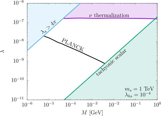
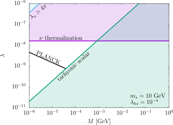
Our numerical results for the total DM relic abundance and the full reaction rates are shown in Fig. 6. We find that the DM yield is dominated by the decay $s\rightarrow\nu\nu$ at temperatures $T\sim m_{s}$ and the required coupling is

\lambda\simeq 1.7\times 10^{-12}\;\sqrt{m_{s}\over M}\;.

(77)

This applies to the regime $m_{s}\gg M$ . In this case, the DM yield $Y$ due to the $s\rightarrow\nu\nu$ decay is independent of $M$ and proportional to $\lambda^{2}$ . Thus, in order to get the right relic abundance, the relation $\lambda\propto 1/\sqrt{M}$ is enforced (while smaller $M$ for the same $\lambda$ lead to under-abundance). We find that these conclusions apply quite generally, beyond the parameter choices of Fig. 6.

Given the correct relic abundance, small and large values of $M$ are excluded by perturbativity and the Higgs mixing or the presence of a tachyonic scalar. Indeed, since $\lambda u=M$ and $m_{s}^{2}=2\lambda_{s}u^{2}$ ,

\lambda_{s}={\lambda^{2}m_{s}^{2}\over 2M^{2}}\;.

(78)

For a fixed relic density and other parameters, $\lambda_{s}\propto 1/M^{3}$ so that at low $M$ it blows up while for large $M$ it violates $4\lambda_{h}\lambda_{s}>\lambda_{hs}^{2}$ .

Since our focus is on freeze–in production of neutrino DM, we exclude significant values of $\lambda$ . These lead to efficient $\nu$ production such that $n_{\nu}$ is close to its equilibrium value. In this case, the reverse process $\nu\nu\rightarrow s$ becomes important and the system tends to equilibrate. Although such a possibility is not excluded by observations, it does not correspond to freeze–in neutrino production.

The approximation $\theta\ll 1$ applies in all of the allowed parameter space: $\theta$ ranges from $10^{-1}$ in the lower right corner to $10^{-5}$ in the upper left corner of the plots. Close to the tachyonic region however, $\theta\sim m_{h}/m_{s}$ or $m_{s}/m_{h}$ such that the relations (14) receive non–negligible corrections. Therefore the tachyonic region border is only approximate.

The stability condition $4\lambda_{s}\lambda_{h}>\lambda_{hs}^{2}$ combined with the right DM yield $Y$ impose a lower bound on $m_{s}$ ,

m_{s}>10^{8}\;\lambda_{hs}^{2/3}M>1~{\rm MeV}\;.

(79)

To get the limit of 1 MeV, we have used $\lambda_{hs}>4\times 10^{-8}$ required for thermalization and the warm DM bound $M>1$ keV (taking the number of SM degrees of freedom at $m_{s}$ to be 10).⁸⁸ 8 The exact lower bound on warm dark matter mass from free streaming [79] depends on its momentum distribution. See, e.g. [80, 81] for recent analyses.

Figure 7: Bose–Einstein vs Maxwell–Boltzmann

s\rightarrow\nu\nu

reaction rates.

The main DM production channel is $s\rightarrow\nu\nu$ . We find that the relativistic effects in this reaction are tangible. Fig. 7 shows that replacing the Bose–Einstein distribution with the Maxwell–Boltzmann one can lead to up to a 65% error in the reaction rate. The Bose–Einstein enhancement is sensitive to the thermal mass: for lower couplings the effect is more pronounced. This is natural since the distribution peaks at low energies while the thermal mass provides a lower bound on how low the energy can be.

5.3 Light $s$ : $m_{s}<2M$

In this case, the main production channel $s\rightarrow\nu\nu$ becomes less significant. The process is kinematically allowed at very high temperatures, when $u=0$ and the Majorana neutrino mass vanishes. It stops after the phase transition to $u\not=0$ . The produced number density is diluted by the subsequent Universe expansion. As a result, the processes like $ss\rightarrow\nu\nu$ and $h\rightarrow\nu\nu$ become equally important or even take over the leading role.

In case of a very light $s$ , there are a number of non–trivial constraints to be observed. In particular, one must make sure that $s$ decays before BBN. Since $s$ cannot decay into neutrinos, the decay proceeds through the mixing with the Higgs. The decay modes and widths are discussed in Appendix B. We impose the constraint $\tau<1$ sec, which ensures that $s$ does not contribute to the relativistic degrees of freedom at BBN and does not destroy light nuclei. Furthermore, for $m_{s}<2m_{\mu}$ , there is a strong constraint on the mixing angle with the Higgs. Rare Kaon decays require $\theta\lesssim 10^{-4}$ [82]. For heavier $s$ , the bound relaxes to $10^{-3}$ or so [83]. Finally, since we are assuming a thermal abundance for $s$ , the Higgs portal coupling must be large enough to ensure thermalization via $h\leftrightarrow ss$ , $\lambda_{hs}>4\times 10^{-8}$ .

Although the available parameter space is quite limited, we find that it is still possible to obtain the right DM relic density. Two examples are shown in Fig. 8. In this case, the strongest constraints are imposed by $\tau_{s}<1$ sec and the absence of tachyons, $4\lambda_{h}\lambda_{s}>\lambda_{hs}^{2}$ . The latter is significant since a light $s$ requires a small $\lambda_{s}$ . In the allowed parameter space, the bound $\theta\lesssim 10^{-4}$ is then satisfied.

As seen in the plots, different reactions dominate at different times. At high temperatures, $s\rightarrow\nu\nu$ dominates but the resulting DM density gets diluted. At later times, $h\rightarrow\nu\nu$ and $ss\rightarrow\nu\nu$ become important. The plateau regions producing the correct DM relic density (Fig. 8, upper row) are associated with $ss\rightarrow\nu\nu$ as the leading (or next-to-leading) production mode. The corresponding rate scales as $T^{4}$ down to temperatures of order $M$ . Thus, the resulting yield satisfies

Y\propto{1\over M}\;.

(80)

Since the required $Y_{\infty}$ also scales as $1/M$ , the PLANCK line corresponds to a plateau in the $(M,\lambda)$ plane. The DM yield associated with the different reactions is shown in the lower row of Fig. 8. The left panel confirms that more than 50% of the yield in the plateau region is indeed provided by $ss\rightarrow\nu\nu$ . We also observe that $s\rightarrow\nu\nu$ makes a significant contribution and tilts the PLANCK line in analogy with Fig. 6.

At somewhat larger masses, the Higgs decay $h\rightarrow\nu\nu$ becomes more important. The amplitude for this process is proportional to $\lambda\,\theta$ which is approximately constant for a fixed $M$ :

\lambda\,\theta\simeq{\lambda_{hs}vM\over m_{h}^{2}}\;.

(81)

Thus, the resulting PLANCK region is almost vertical in the $(M,\lambda)$ plane. The lower right panel of Fig. 8 shows that the dominant DM yield is produced at electroweak temperatures via $h\rightarrow\nu\nu$ . To the left of the PLANCK curve, our DM is under-abundant.

The neutrino thermalization constraint of Fig. 2 is not directly applicable here since the channel $s\rightarrow\nu\nu$ is not available. We find that, in the allowed parameter region, $n_{\nu}$ is below its equilibrium value so the neutrinos can be treated as non–thermal.

6 Sterile neutrino production II: non–thermal $s$

It is possible that $s$ never reaches thermal equilibrium either due to its large mass or due to its small couplings. In general, there is a variety of non–thermal $s$ –production mechanisms in the Early Universe. Its direct coupling to an inflaton would lead to perturbative and/or non–perturbative production, e.g. via parametric resonance [84]. Furthermore, light scalar field fluctuations during inflation generate an $s$ –condensate which then decays into $s$ –quanta. However, these mechanisms are sensitive to further details of the complete UV model, for instance, to the Hubble rate during inflation [85]. In particular, for small Hubble rates such contributions are suppressed. In what follows, we focus on $s$ –production from a Standard Model thermal bath and assume that the other sources are subdominant.

6.1 Heavy $s$

If $s$ is very heavy while the temperature is not high enough, the singlet does not thermalize and can be integrated out. DM production proceeds through Higgs annihilation $hh\rightarrow\nu\nu$ and decay $h\rightarrow\nu\nu$ due to the Higgs–singlet mixing. We find that the decay mode dominates for the parameter values of interest.

It is instructive to consider the channel $hh\rightarrow\nu\nu$ separately. When this mode dominates, one recovers the so–called “UV freeze–in” scenario. In this case, the DM abundance is sensitive to the maximal temperature $T_{0}<T_{c}^{u}$ . The Boltzmann equation at high $T$ reads

T{dn\over dT}-3n+{8\Gamma_{22}(hh\rightarrow\nu\nu)\over H}=0\;,

(82)

where the factor of 8 takes into account 4 Higgs d.o.f. above the EW transition scale. Since $\Gamma_{22}\propto T^{6}$ at high $T$ ,

n(T)\propto T_{0}T^{3}\;.

(83)

As a result, the DM yield $Y=n/s_{\rm SM}\propto T_{0}$ is determined by the UV end of the evolution. This is unlike the usual freeze–in scenario where the IR behaviour is more important.

Although the decay channel $h\rightarrow\nu\nu$ opens up only below the EW breaking scale, numerically it turns out to be more important and the sensitivity of the DM abundance to $T_{0}$ is weak. Our numerical results are presented in Fig. 9 which shows the regions with the right relic abundance. The DM production amplitude is proportional to the combination $\lambda\theta$ which is fixed for a fixed $M$ . This makes the production rate independent of $\lambda$ and the PLANCK region vertical in the $(M,\lambda)$ plane. As before, our DM is under-abundant to the left of the PLANCK line.

The Higgs portal coupling required for the correct DM relic abundance can be approximated by (ignoring the phase transition complications):

\lambda_{hs}\simeq\;{m_{s}^{2}\over M^{3/2}}~{4\times 10^{-14}\over\sqrt{\rm GeV}}

(84)

for $g_{*}\simeq 107$ . We have verified that the neutrino thermalization constraint is insignificant and $n_{\nu}$ is below its equilibrium value.

In the allowed parameter space, the mixing angle ranges from $10^{-2}$ to $10^{-6}$ . As before, the $\theta^{2}$ corrections become significant close to the tachyonic region border.

6.2 Small couplings: freeze–in production of $s$

Here we consider the possibility that the $\lambda_{hs}$ and $\lambda_{s}$ couplings are so small that $s$ never reaches thermal equilibrium (see, e.g. [86] for early work). Assuming that the initial abundance of $s$ is zero or negligibly small, the $s$ quanta are produced by the Higgs thermal bath via the usual freeze–in mechanism. Subsequently, they decay into sterile neutrinos leading to the required DM abundance. Due to the $s-h$ mixing, $s$ decays also produce SM particles, yet this gives only a small correction to the entropy since the density of $s$ is far below its equilibrium value.

There are a few $s$ –production channels: $hh\rightarrow ss$ , $h\rightarrow ss$ and $hh\rightarrow s$ , where the last two reactions are possible only below the corresponding critical temperatures. $hh\rightarrow s$ is a new reaction type, not considered before. Hence, it is instructive to consider it in more detail.

6.2.1 $hh\rightarrow s$ rate

The general expression for the reaction rate reads

\Gamma_{21}=\int\left(\prod_{i\in a}{d^{3}{\bf p}_{i}\over(2\pi)^{3}2E_{i}}f(p_{i})\right)~{d^{3}{\bf p}_{f}\over(2\pi)^{3}2E_{f}}|{\cal M}_{2\rightarrow 1}|^{2}~(2\pi)^{4}\delta^{4}(p_{1}+p_{2}-p_{f}).

(85)

Here $|{\cal M}_{2\rightarrow 1}|^{2}$ includes $1/2$ from the phase space symmetry of the initial state.

Performing the angular integrals as before and using

\int{d^{3}{\bf p_{f}}\over(2\pi)^{3}2E_{f}}\;(2\pi)^{4}\delta(p_{1}+p_{2}-p_{f})={\pi\over 2m_{s}}\;\delta(E-m_{s}/2)\;

(86)

as well as $|{\cal M}_{2\rightarrow 1}|^{2}=1/2\times\lambda_{hs}^{2}u^{2}$ , we find

\Gamma_{21}={\lambda_{hs}^{2}u^{2}m_{s}T\over 32\pi^{3}}\theta(m_{s}-2m_{h})\int_{0}^{\infty}d\eta{\sinh\eta\over e^{m_{s}\cosh\eta\over T}-1}\;\ln{\sinh{m_{s}\cosh\eta+\sqrt{m_{s}^{2}-4m_{h}^{2}}\sinh\eta\over 4T}\over\sinh{m_{s}\cosh\eta-\sqrt{m_{s}^{2}-4m_{h}^{2}}\sinh\eta\over 4T}}\;.

(87)

This expression is valid for a single Higgs d.o.f.

6.2.2 $h\rightarrow ss$ and $hh\rightarrow ss$ rates

These reaction rates have been computed in [48]. For a single Higgs d.o.f., the results read

$\displaystyle\Gamma_{12}$	$\displaystyle=$	$\displaystyle{\lambda_{hs}^{2}v^{2}m_{h}^{2}\over 64\pi^{3}}\sqrt{1-{4m_{s}^{2}\over m_{h}^{2}}}\;\int_{1}^{\infty}dx\;{\sqrt{x^{2}-1}\over e^{{m_{h}\over T}x}-1}\;,$
$\displaystyle\Gamma_{22}$	$\displaystyle=$	$\displaystyle{1\over 2!2!}\;{\lambda_{hs}^{2}T\over 16\pi^{5}}$	(88)
	$\displaystyle\times$	$\displaystyle\int_{m_{h}}^{\infty}dE~E\sqrt{E^{2}-m_{s}^{2}}\int_{0}^{\infty}d\eta{\sinh\eta\over e^{{2E\over T}\cosh\eta}-1}~\ln{\sinh{E\cosh\eta+\sqrt{E^{2}-m_{h}^{2}}\sinh\eta\over 2T}\over\sinh{E\cosh\eta-\sqrt{E^{2}-m_{h}^{2}}\sinh\eta\over 2T}}\;,$	(88)

where $E$ is half the CM energy and we have factored out the symmetry factor $1/2!2!$ stemming from 2 identical particles in the initial and final states.

6.2.3 Results

The number density of the $s$ –quanta is calculated according to

\dot{n}_{s}+3n_{s}H=2\hat{\Gamma}_{12}(h\rightarrow ss)+2\hat{\Gamma}_{22}(hh\rightarrow ss)+\hat{\Gamma}_{21}(hh\rightarrow s)\;,

(89)

where

	$\displaystyle\hat{\Gamma}_{12}(h\rightarrow ss)=\theta(T_{c}^{v}-T)\;\Gamma_{12}(h\rightarrow ss)\;,$		(90)
	$\displaystyle\hat{\Gamma}_{22}(hh\rightarrow ss)=(4-3\theta(T_{c}^{v}-T))\;\Gamma_{22}(hh\rightarrow ss)\;,$		(91)
	$\displaystyle\hat{\Gamma}_{21}(hh\rightarrow s)=(4-3\theta(T_{c}^{v}-T))\;\Gamma_{21}(hh\rightarrow s)\;.$		(92)

Here the $\theta$ –functions account for the EW phase transition and the change in the number of the Higgs d.o.f. We neglect the dependence on $T_{c}^{u}$ since $s$ is not thermalized and $\lambda_{hs}$ is very small.

Since there is no significant back reaction of the produced $s$ quanta on the thermal bath nor substantial entropy production via $s$ –decay, the total DM yield can then be computed as the $s$ –yield times the branching ration for the $s$ decay into dark matter,

Y_{\nu}=2\;Y_{s}\;{\rm BR}(s\rightarrow\nu\nu)\;.

(93)

The $s$ decay width into the SM particles is given in Appendix B.

Figure 10:

\lambda

M

generating the correct relic DM relic density (“PLANCK”) for a non–thermal

s

. Here

s

is produced by the freeze–in mechanism via the Higgs thermal bath. In the excluded regions, the freeze–in calculations become unreliable due to efficient

hh\leftrightarrow s

ss\rightarrow ssss

processes leading to thermalization.

We compute the number density of $s$ via freeze–in calculations. Thus, it is important to observe the non–thermalization constraints. For a given $\lambda$ , an increase in $M$ implies an increase in $u$ , which makes $s$ production via $hh\rightarrow s$ more efficient and can lead to thermalization. A competitive constraint, which becomes stronger for light $s$ , is imposed by vacuum stability, $4\lambda_{s}\lambda_{h}>\lambda_{hs}^{2}$ . Furthermore, in regions with a substantial $\lambda_{s}$ , the process $ss\rightarrow ssss$ becomes efficient and can lead to self–thermalization. We exclude these as well. An additional Kaon physics constraint $\theta<10^{-4}$ applies for a very light $s$ , $m_{s}<200$ MeV. We find, however, that it is satisfied automatically.

Our numerical results are presented in Fig. 10. The behaviour of the PLANCK curve can be understood as follows. The factors that determine the neutrino abundance are $Y_{s}$ and the decay branching fraction for $s\rightarrow\nu\nu$ . Consider first the regime $m_{s}\gg m_{h}$ . In this case, $Y_{s}$ is determined by the fusion process $hh\rightarrow s$ , whose rate is proportional to $u^{2}=M^{2}/\lambda^{2}$ . It terminates at temperatures of order $m_{s}\gg M$ , so the $s$ –yield scales simply as $M^{2}/\lambda^{2}$ with $M$ and $\lambda$ . Now there are two options: $s$ –decay can be dominated either by the sterile neutrino mode or by the SM channels. For $\Gamma(s\rightarrow\nu\nu)\gg\Gamma(s\rightarrow{\rm SM})$ , the branching ratio ${\rm BR}(s\rightarrow\nu\nu)$ can be approximated by 1. Since $Y_{\infty}\propto 1/M$ , the PLANCK line then satisfies $\lambda\propto M^{3/2}$ . In the opposite case $\Gamma(s\rightarrow\nu\nu)\ll\Gamma(s\rightarrow{\rm SM})$ , the branching ratio scales with $\lambda$ and $M$ as ${\Gamma(s\rightarrow\nu\nu)\over\Gamma(s\rightarrow{\rm SM})}\propto\lambda^{2}/\theta^{2}\propto\lambda^{4}/M^{2}$ at $m_{s}\gg M$ . This results in $\lambda\propto M^{-1/2}$ . Thus, we have:

$\displaystyle m_{s}\gg m_{h}:$		(94)
	$\displaystyle\lambda\propto M^{3/2}~~~{\rm for~larger~}\lambda$
	$\displaystyle\lambda\propto M^{-1/2}~~{\rm for~smaller~}\lambda$

This scaling is observed in the left panel of Fig. 10.

For $m_{s}\ll m_{h}$ , the $s$ –abundance is dominated by $h\rightarrow ss$ . If $s$ decays predominantly into neutrinos, the DM yield is independent of $\lambda$ . Otherwise, it is proportional to $\lambda^{4}/M^{2}$ . Thus, we get

$\displaystyle m_{s}\ll m_{h}:$		(95)
	$\displaystyle M={\rm const}~~{\rm for~larger~}\lambda$
	$\displaystyle\lambda\propto M^{1/4}~~~~{\rm for~smaller~}\lambda$

This behaviour is seen in the right panel of the figure. In both panels, DM is under-abundant to the left of (or below) the PLANCK curve.

We see that quite large values of $\lambda$ up to $10^{-3}$ are consistent with all of the constraints. One may worry that the neutrinos would thermalize via $s\leftrightarrow\nu\nu$ at such a large coupling. However, the density of $s$ is much lower than its equilibrium value and this reaction does not increase the number of $s$ –quanta, while $\nu\rightarrow\nu s$ is not allowed kinematically and $\nu\nu\rightarrow ss$ is suppressed. Thus, the system is not expected to thermalize.

For a very light $s$ , the BBN constraint on the lifetime of $s$ becomes significant: at small $\lambda$ , it decays mostly into the photons and electrons which affect the abundance of light elements unless $\tau_{s}<1$ sec.

Finally, we find that the mixing angle is very small in all the cases considered and its effects can be neglected.

6.2.4 On electroweak phase transition effects

The EW phase transition can have an important impact on the DM abundance. The Higgs mass reduction close to the transition opens up the fusion channel

hh\rightarrow s

even if this process is forbidden kinematically at other temperatures. It is operative if $2m_{h}(T\simeq T_{c}^{v})<m_{s}$ , while its efficiency depends on the nature of the transition. (An analogous effect in a different setting was considered in [87].)

In this work, we are interested in small couplings. Then, the electroweak phase transition corresponds either to a second order phase transition or a crossover. In the former case, the Higgs becomes massless at the critical temperature, while at the crossover it remains massive. Perturbative analysis is insufficient to distinguish the two: what appears as a second order transition typically corresponds to a crossover, as established by lattice simulations. The full analysis of the singlet scalar extension is not yet available, although for a heavy singlet or EW triplet, the nature of the transition has been determined in [88, 89, 90]. The second order transition is found to occur in special cases, while a crossover is very common at weak coupling. This is to be contrasted with perturbative calculations (see e.g. [91]). Similar results are expected to apply in the light singlet or triplet case.⁹⁹ 9 We thank Lauri Niemi for sharing some of his results.

Although the Higgs does not turn massless at the crossover, its mass gets significantly reduced. In the SM, this reduction reaches an order of magnitude at the (pseudo-)critical temperature [92] (see also earlier work [93, 94]). Since we are mostly interested in very small Higgs portal couplings, the presence of the singlet is not expected to change the nature of the transition. Thus, we may assume $m_{h}(T_{c}^{v})\sim 10$ GeV as in the SM.

Figure 11: Left: Estimate of the

hh\rightarrow s

reaction rate at the EW crossover with

m_{h}(T_{c})=10

GeV. The

s-h

mixing is set to zero. Right: Bose–Einstein enhancement factor for

hh\rightarrow s

at the 2d order EW phase transition.

To estimate the efficiency of the fusion mode, let us consider a simplified case of zero $s-h$ mixing and employ a simple parametrization¹⁰¹⁰ 10 This parametrization is inspired by the perturbative description of the 2d order phase transition, while it does not quite hold non–perturbatively. Nevertheless, it is acceptable for our estimate since the production is dominated by $T\simeq T_{c}$ where the Higgs mass is almost constant.

	$\displaystyle m_{h}^{2}(T)=c(T^{2}-T_{c}^{2})+m_{h}^{2}(T_{c})~~~{\rm for}~~T>T_{c}~,$
	$\displaystyle m_{h}^{2}(T)=2c(T^{2}_{c}-T^{2})+m_{h}^{2}(T_{c})~~{\rm for}~~T<T_{c}~,$		(96)

where $T_{c}\equiv T_{c}^{v}$ is the EW critical temperature and $c$ is a constant fixed by requiring $m_{h}(0)=125$ GeV. Taking a simple perturbative estimate for $T_{c}$ , one can then calculate the fusion rate. The resulting $hh\rightarrow s$ rate for a representative parameter set is shown in Fig. 11, left panel.

We find that this effect $alone$ can account for all of the observed dark matter. Although short, the fusion is intense enough to produce numerous $s$ –quanta which subsequently decay into sterile neutrinos. As one gets closer to the 2d order transition (at larger $\lambda_{hs}$ ), the Bose–Einstein enhancement becomes more pronounced. This is illustrated in Fig. 11, right panel. When both $m_{h}(T_{c})$ and $m_{s}$ are far smaller than the temperature, the Bose–Einstein enhancement factor can reach orders of magnitude.

The fusion mode can be more efficient than the decay $h\rightarrow ss$ . Indeed, the fusion rate grows as $u^{2}$ which can be very large, while the decay rate remains constant for a fixed $m_{s}$ . Thus, the thermalization constraints in Figs. 3,4 due to the fusion mode extend to $m_{s}<2m_{h}$ as well and can be more stringent then those due the decay, depending on $u$ . However, in view of the uncertainties, we have not included these to be conservative.

We note that our approximation breaks down at $m_{s}\sim m_{h}$ , i.e. when the mixing angle becomes significant. As pointed out in [77], the resonantly enhanced $s-h$ mixing leads to additional scalar production. With present tools, it is however difficult to estimate its efficiency and we leave it for future work. We stress that the fusion mechanism considered here is intrinsically different and operative for small (and zero) mixing as long as $2m_{h}(T)<m_{s}$ .

7 Conclusion

The lightest sterile neutrino is an attractive dark matter candidate. Although it is not stable, its longevity is guaranteed by its small mass and a small sterile–active mixing angle. In this work, we explore the mass range up to 1 GeV. In this case, tiny mixing angles are necessary which one can justify by a flavor–dependent (neutrino parity) symmetry.

We have focused on the scenario where the Majorana masses are entirely due to a VEV of a real scalar. This is enforced by a discrete lepton number symmetry, which is broken spontaneously by the scalar VEV. The scalar is then only allowed to couple to the SM quadratically through the Higgs portal.

Since the neutrinos can be very weakly coupled, the natural (but generally not unique) dark matter production mechanism is the freeze–in. We have analyzed freeze–in production of sterile neutrinos ( $\nu$ ) from the Higgs and singlet scalar ( $s$ ) thermal bath in different regimes. These are summarized in the following table.

	regime	dominant modes
thermal $s$
	$m_{s}>2M$	$s\rightarrow\nu\nu$
	$m_{s}<2M$	$ss\rightarrow\nu\nu$ , $h\rightarrow\nu\nu$ , $s\rightarrow\nu\nu$
non–thermal $s$
	heavy $s$	$h\rightarrow\nu\nu$
	feebly coupled $s$	$s\rightarrow\nu\nu$

In all of these cases, the observed DM relic density can be obtained. For the sterile neutrino mass range (1 keV, 1 GeV), we find that the requisite scalar–neutrino coupling varies between $10^{-10}$ and $10^{-3}$ . Our analysis takes into account the relativistic reaction rates with the Bose–Einstein distribution function, thermal masses and main effects of the phase transitions. All of these factors make an important impact on the final results. As byproducts, we have derived relativistic rates for asymmetric reactions as well as non–thermalization constraints on sterile neutrinos and the Higgs portal scalar.

We find a number of interesting effects which deserve further study. In particular, a light scalar can be copiously produced close to the EW phase transition/crossover through the fusion mode $hh\rightarrow s$ . Subsequent decay of the scalar into sterile neutrinos can account for all of the dark matter. However, the specifics of this mechanism require understanding non–perturbative dynamics close to the critical temperature.

The dark matter candidate studied here is long–lived. Its production mechanism is independent of the sterile–active mixing $\Theta$ , hence there is vast parameter space $(\Theta,M)$ where dark matter decay can lead to an observable signal, e.g. in the form of monochromatic X- or gamma rays. The intensity of the signal is correlated with the dark matter density.

Acknowledgements. OL is indebted to Mark Hindmarsh, Lauri Niemi and Aleksi Vuorinen for invaluable discussions. VDR acknowledges financial support by the SEJI/2018/033 grant, funded by Generalitat Valenciana and partial support by the Spanish grants FPA2017-85216-P and FPA2017-90566-REDC (Red Consolider MultiDark). DK is supported by the National Science Centre, Poland, research grant No. 2015/18/A/ST2/00748. This work was made possible by Institut Pascal at Université Paris-Saclay with the support of the P2I and SPU research departments and the P2IO Laboratory of Excellence (program “Investissements d’avenir” ANR-11-IDEX-0003-01 Paris-Saclay and ANR-10-LABX-0038), as well as the IPhT. TT acknowledges funding from the Natural Sciences and Engineering Research Council of Canada (NSERC). Numerical computation in this work was carried out at the Yukawa Institute Computer Facility.

Appendix A Leading thermal corrections

In this Appendix, we summarize the most important thermal corrections to the effective potential in our model.

The tree-level effective scalar potential, written in terms of the vevs $v,u$ reads

V^{0}=\frac{\lambda_{h}}{4}v^{4}+\frac{\lambda_{hs}}{4}v^{2}u^{2}+\frac{\lambda_{s}}{4}u^{4}+\frac{1}{2}\;\mu_{h}^{2}\,v^{2}+\frac{1}{2}\mu_{s}^{2}\,u^{2}\,.

(97)

The zero-temperature one-loop correction to effective potential is given by the Coleman-Weinberg correction [95], which in the $\overline{MS}$ renormalisation scheme is

V^{1}=\sum_{\alpha}\frac{n_{\alpha}}{64\pi^{2}}m^{4}_{\alpha}(v,u)\left(\log\frac{m^{2}_{\alpha}(v,u)}{Q^{2}}-C_{\alpha}\right)\,.

(98)

Here $\alpha$ runs over all dominant degrees of freedom: $t,~W,~Z,~G^{\pm,0}$ and $\chi_{1,2}$ (the mass eigenstates of the scalar fields $h$ and $s$ ). The number of d.o.f. $n_{\alpha}$ are given by $n_{t}=-12,~n_{W}=6,~n_{Z}=3,~n_{G}=3,~n_{\chi_{1,2}}=1$ (it includes a minus sign for fermions). $m^{2}_{\alpha}(v,u)$ are the field-dependent masses-squared, $C_{\alpha}=3/2~(5/6)$ for scalars (gauge bosons) and $Q$ is the renormalisation scale. In our calculations, we take $Q$ to be the particle masses in the vacuum at zero $T$ . The field-dependent masses are:

$\displaystyle m_{t}^{2}(v,u)$	$\displaystyle=$	$\displaystyle y_{t}^{2}\frac{v^{2}}{2}~,$	(99)
$\displaystyle m_{W}^{2}(v,u)$	$\displaystyle=$	$\displaystyle g^{2}\frac{v^{2}}{4}~,$	(100)
$\displaystyle m_{Z}^{2}(v,u)$	$\displaystyle=$	$\displaystyle(g^{2}+g^{\prime 2})\frac{v^{2}}{4}~,$	(101)
$\displaystyle m_{G^{0}}^{2}(v,u)=m_{G^{\pm}}^{2}(v,u)$	$\displaystyle=$	$\displaystyle v^{2}\lambda_{h}+\frac{\lambda_{hs}u^{2}}{2}+\mu_{h}^{2}~,$	(102)
$\displaystyle m_{\chi_{1,2}}^{2}(v,u)$	$\displaystyle=$	$\displaystyle v^{2}\lambda_{h}+\lambda_{s}u^{2}\pm\sqrt{v^{4}\lambda_{h}^{2}+v^{2}u^{2}(\lambda_{hs}^{2}-2\lambda_{h}\lambda_{s})+\lambda_{s}^{2}u^{4}}.$	(103)

The temperature effects are conveniently split into a one-loop temperature–dependent part $V^{1,T}$ and the ring corrections $V^{T}_{\rm ring}$ [96, 97]. The former is given by the one-loop thermal integral

V^{1,T}(T)=\sum_{\alpha}\frac{n_{\alpha}T^{4}}{2\pi^{2}}\mathcal{I}_{b,f}\left(\frac{m_{\alpha}^{2}(v,u)}{T^{2}}\right)\;,

(104)

where

\mathcal{I}_{b,f}\left(\frac{m_{\alpha}^{2}(v,u)}{T^{2}}\right)=\int_{0}^{\infty}dx~x^{2}\log\left[1\pm e^{-\sqrt{x^{2}+y^{2}}}\right]\,,~y^{2}=m^{2}_{\alpha}(v,u)/T^{2}\;,

(105)

with the plus (minus) sign for fermions (bosons), respectively. The ring contribution is present only for bosons (gauge bosons, scalars and Goldstones):

	$\displaystyle V^{T}_{{}_{\rm ring}}$	$\displaystyle=$	$\displaystyle-\frac{T}{12\pi}\biggl\{{\rm Tr}\left[(m_{gb}^{2}+\Pi_{gb})^{3/2}-(m_{gb}^{2})^{3/2}\right]+{\rm Tr}\left[(m_{\rm\chi}^{2}+\Pi_{\rm\chi})^{3/2}-(m_{\rm\chi}^{2})^{3/2}\right]$		(106)
		$\displaystyle+$	$\displaystyle n_{G}\left[(m_{G}^{2}+\Pi_{G})^{3/2}-(m_{G}^{2})^{3/2}\right]\biggr\}\,,$		(106)

where $m_{\chi}$ is the tree level scalar mass mixing matrix whose eigenstates are $\chi_{1,2}$ . The squared mass mixing matrix for the electroweak gauge bosons is:

\displaystyle m_{gb}^{2}

\displaystyle=

\displaystyle\left(\begin{array}[]{cccc}\frac{g^{2}}{4}v^{2}&0&0&0\\ 0&\frac{g^{2}}{4}v^{2}&0&0\\ 0&0&\frac{g^{2}}{4}v^{2}&-\frac{gg^{\prime}}{4}v^{2}\\ 0&0&-\frac{gg^{\prime}}{4}v^{2}&\frac{g^{\prime 2}}{4}v^{2}\\ \end{array}\right)\,.

The $\Pi_{i}$ are the thermally corrected contributions to the masses [97, 98, 99]:

$\displaystyle\Pi_{gb}$	$\displaystyle=$	$\displaystyle\frac{11}{6}T^{2}{\rm diag}\left(g^{2},\;g^{2},\;g^{2},\;g^{\prime 2}\right)~,$
$\displaystyle\Pi_{\chi}$	$\displaystyle=$	$\displaystyle\frac{1}{4}T^{2}{\rm diag}\left[\left(\frac{3}{4}g^{2}+\frac{1}{4}g^{\prime 2}+2\lambda_{h}+y_{t}^{2}+\frac{4\lambda_{hs}}{3}\right),\lambda_{s}+\frac{1}{3}\lambda_{hs}\right]~,$
$\displaystyle\Pi_{G}$	$\displaystyle=$	$\displaystyle\frac{1}{4}T^{2}\left(\frac{3}{4}g^{2}+\frac{1}{4}g^{\prime 2}+2\lambda_{h}+y_{t}^{2}+\frac{4\lambda_{hs}}{3}\right)\,.$	(112)

The effective potential is then given by the sum of all of the above contributions:

V^{T}_{\rm eff}=V^{0}+V^{1}+V^{1,T}+V^{T}_{{}_{\rm ring}}\,.

(113)

In our analysis, we keep only the most important terms. We assume $V^{1}$ to be negligible at high temperatures and use a $1/T$ expansion of the integrals in Eq. 105 [96]:

	$\displaystyle\mathcal{I}_{b}\left(\frac{m}{T}\right)$	$\displaystyle\approx$	$\displaystyle-\frac{\pi^{4}}{45}+\frac{\pi^{2}}{12}\frac{m^{2}}{T^{2}}\,,$
	$\displaystyle\mathcal{I}_{f}\left(\frac{m}{T}\right)$	$\displaystyle\approx$	$\displaystyle\frac{7\pi^{4}}{360}-\frac{\pi^{2}}{24}\frac{m^{2}}{T^{2}}\,.$		(114)

It further proves convenient to use the expansion of the trace:

\left[(m_{i}^{2}+\Pi_{i})^{3/2}-(m_{i}^{2})^{3/2}\right]\approx\Pi_{i}^{3/2}+\frac{3}{2}\rm Tr\left[m_{i}^{2}\sqrt{\Pi_{i}}\right]\,.

(115)

Ignoring all field–independent terms, which shift the potential by a temperature dependent constant, we find that the ring corrections are of higher order in the couplings ( $\sim g^{3}$ ) and can be neglected. The effective potential takes the form:

V^{T}_{\rm eff}=\frac{\lambda_{h}}{4}v^{4}+\frac{\lambda_{hs}}{4}v^{2}u^{2}+\frac{\lambda_{s}}{4}u^{4}+\frac{1}{2}\left[(c_{h}T^{2}+\mu_{h}^{2})v^{2}+(c_{s}T^{2}+\mu_{s}^{2})u^{2}\right]\,,

(116)

with $c_{h}=\frac{1}{4}\left(\frac{2g^{2}}{4}+\frac{g^{2}+g^{\prime 2}}{4}+y_{t}^{2}+2\lambda_{h}+\frac{\lambda_{hs}}{6}\right)$ and $c_{s}=\frac{1}{4}\left(\lambda_{s}+\frac{2}{3}\lambda_{hs}\right)$ .

Appendix B $s$ decay partial widths

The real scalar $s$ interacts with the SM particles via its mixing with the Higgs. Its decay rates can be obtained from the Higgs ones [100] by including the factor $\sin^{2}\theta$ . For $0.1~{\rm GeV}<m_{s}\lesssim 90$ GeV, we use the Higgs total decay width given in Refs. [101, 102]. For masses $90~{\rm GeV}<m_{s}<1000$ GeV, we use the results of Ref. [103]. Finally, for $m_{s}>1$ TeV, we scale the width up according to $m_{s}^{3}$ .

If $m_{s}<2M$ and $M$ is in the keV range, $s$ will decay only to photons. In the calculation of the partial decay width into photons, we follow [104]:

\Gamma(s\to\gamma\gamma)=\frac{G_{F}\alpha^{2}m_{s}^{3}\sin^{2}\theta}{128\sqrt{2}\pi^{3}}\Bigg|\sum_{f}N^{f}_{c}Q_{f}^{2}A_{f}(\tau_{f})+N^{W}_{c}Q_{W}^{2}A_{W}(\tau_{W})\Bigg|^{2},

(117)

where the sum runs over fermions and $W$ inside the loop. In this expression, $N^{f(W)}_{c}=3(1)$ , $Q_{i}$ is the charge and $G_{F}$ is the Fermi coupling constant. We define the following mass ratio

\tau_{\rm x}=\frac{m_{s}^{2}}{4m_{\rm x}^{2}}\,

(118)

and the loop functions

	$\displaystyle A_{f}(\tau)$	$\displaystyle=2(\tau+(\tau-1)f(\tau))/\tau^{2},$		(119)
	$\displaystyle A_{W}(\tau)$	$\displaystyle=-(2\tau^{2}+3\tau+3(2\tau-1)f(\tau))/\tau^{2},$		(120)

with

f(\tau)=\begin{cases}\text{arcsin}^{2}\sqrt{\tau}\hskip 28.45274pt&\text{for}\,\,\tau\leq 1,\\ -\frac{1}{4}\left(\log\frac{1+\sqrt{1-\tau^{-1}}}{1-\sqrt{1-\tau^{-1}}}-i\pi\right)^{2}&\text{for}\,\,\tau>1.\end{cases}

(121)

Note that $\sin\theta$ depends on $m_{s}$ :

\sin 2\theta=\frac{M}{\lambda}\;\frac{2\lambda_{hs}v}{m_{s}^{2}-m_{h}^{2}}\,.

(122)

Figure 12: The total SM decay width of

s

and

\Gamma(s\rightarrow\nu\nu)

for

\lambda=10^{-5}

\lambda_{hs}=10^{-8}

and

M=1

GeV.

For heavier $m_{s}$ , the scalar will also decay into other SM particles. Besides the SM channels, $s$ has another important decay mode $s\rightarrow\nu\nu$ . The corresponding decay width reads

\Gamma(s\to\nu\nu)=\lambda^{2}\frac{m_{s}}{16\pi}\left(1-4\frac{M^{2}}{m_{s}^{2}}\right)^{3/2}.

(123)

Fig. 12 shows the total SM decay width and $\Gamma(s\to\nu\nu)$ as a function of $m_{s}$ with other parameters fixed at some representative values. While the neutrino width grows with $m_{s}$ , the SM decays get suppressed due to the decrease in the mixing angle $\theta\propto 1/m_{s}^{2}$ . The spike in $\Gamma_{s}$ around $m_{h}\simeq m_{s}$ is due to the sharp increase in $\sin\theta$ . In this region, our approximations are unreliable.

References

[1] P. Minkowski, “ $\mu\to e\gamma$ at a Rate of One Out of $10^{9}$ Muon Decays?,” Phys. Lett. 67B (1977) 421–428.
[2] M. Gell-Mann, P. Ramond, and R. Slansky, “Complex Spinors and Unified Theories,” Conf. Proc. C790927 (1979) 315–321, arXiv:1306.4669 [hep-th].
[3] T. Yanagida, “Horizontal gauge symmetry and masses of neutrinos,” Conf. Proc. C7902131 (1979) 95–99.
[4] R. N. Mohapatra and G. Senjanovic, “Neutrino Mass and Spontaneous Parity Nonconservation,” Phys. Rev. Lett. 44 (1980) 912. [,231(1979)].
[5] J. Schechter and J. W. F. Valle, “Neutrino Masses in SU(2) x U(1) Theories,” Phys. Rev. D22 (1980) 2227.
[6] G. Lazarides, Q. Shafi, and C. Wetterich, “Proton Lifetime and Fermion Masses in an SO(10) Model,” Nucl. Phys. B181 (1981) 287–300.
[7] S. Dodelson and L. M. Widrow, “Sterile-neutrinos as dark matter,” Phys. Rev. Lett. 72 (1994) 17–20, arXiv:hep-ph/9303287 [hep-ph].
[8] A. Boyarsky, A. Neronov, O. Ruchayskiy, and M. Shaposhnikov, “Constraints on sterile neutrino as a dark matter candidate from the diffuse x-ray background,” Mon. Not. Roy. Astron. Soc. 370 (2006) 213–218, arXiv:astro-ph/0512509 [astro-ph].
[9] U. Seljak, A. Makarov, P. McDonald, and H. Trac, “Can sterile neutrinos be the dark matter?,” Phys. Rev. Lett. 97 (2006) 191303, arXiv:astro-ph/0602430 [astro-ph].
[10] A. Boyarsky, J. Nevalainen, and O. Ruchayskiy, “Constraints on the parameters of radiatively decaying dark matter from the dark matter halo of the Milky Way and Ursa Minor,” Astron. Astrophys. 471 (2007) 51–57, arXiv:astro-ph/0610961 [astro-ph].
[11] A. Boyarsky, A. Neronov, O. Ruchayskiy, M. Shaposhnikov, and I. Tkachev, “Where to find a dark matter sterile neutrino?,” Phys. Rev. Lett. 97 (2006) 261302, arXiv:astro-ph/0603660 [astro-ph].
[12] A. Boyarsky, D. Iakubovskyi, O. Ruchayskiy, and V. Savchenko, “Constraints on decaying Dark Matter from XMM-Newton observations of M31,” Mon. Not. Roy. Astron. Soc. 387 (2008) 1361, arXiv:0709.2301 [astro-ph].
[13] A. Boyarsky, D. Malyshev, A. Neronov, and O. Ruchayskiy, “Constraining DM properties with SPI,” Mon. Not. Roy. Astron. Soc. 387 (2008) 1345, arXiv:0710.4922 [astro-ph].
[14] H. Yuksel, J. F. Beacom, and C. R. Watson, “Strong Upper Limits on Sterile Neutrino Warm Dark Matter,” Phys. Rev. Lett. 101 (2008) 121301, arXiv:0706.4084 [astro-ph].
[15] A. Boyarsky, J. Lesgourgues, O. Ruchayskiy, and M. Viel, “Lyman-alpha constraints on warm and on warm-plus-cold dark matter models,” JCAP 0905 (2009) 012, arXiv:0812.0010 [astro-ph].
[16] Fermi-LAT Collaboration, M. Ackermann et al., “Updated search for spectral lines from Galactic dark matter interactions with pass 8 data from the Fermi Large Area Telescope,” Phys. Rev. D91 no. 12, (2015) 122002, arXiv:1506.00013 [astro-ph.HE].
[17] K. Perez, K. C. Y. Ng, J. F. Beacom, C. Hersh, S. Horiuchi, and R. Krivonos, “Almost closing the $\nu$ MSM sterile neutrino dark matter window with NuSTAR,” Phys. Rev. D95 no. 12, (2017) 123002, arXiv:1609.00667 [astro-ph.HE].
[18] M. Drewes et al., “A White Paper on keV Sterile Neutrino Dark Matter,” JCAP 1701 (2017) 025, arXiv:1602.04816 [hep-ph].
[19] X.-D. Shi and G. M. Fuller, “A New dark matter candidate: Nonthermal sterile neutrinos,” Phys. Rev. Lett. 82 (1999) 2832–2835, arXiv:astro-ph/9810076 [astro-ph].
[20] K. Abazajian, G. M. Fuller, and M. Patel, “Sterile neutrino hot, warm, and cold dark matter,” Phys. Rev. D64 (2001) 023501, arXiv:astro-ph/0101524 [astro-ph].
[21] T. Asaka, S. Blanchet, and M. Shaposhnikov, “The nuMSM, dark matter and neutrino masses,” Phys. Lett. B631 (2005) 151–156, arXiv:hep-ph/0503065 [hep-ph].
[22] T. Asaka, M. Laine, and M. Shaposhnikov, “Lightest sterile neutrino abundance within the nuMSM,” JHEP 01 (2007) 091, arXiv:hep-ph/0612182 [hep-ph]. [Erratum: JHEP02,028(2015)].
[23] L. Canetti, M. Drewes, and M. Shaposhnikov, “Sterile Neutrinos as the Origin of Dark and Baryonic Matter,” Phys. Rev. Lett. 110 no. 6, (2013) 061801, arXiv:1204.3902 [hep-ph].
[24] L. Canetti, M. Drewes, T. Frossard, and M. Shaposhnikov, “Dark Matter, Baryogenesis and Neutrino Oscillations from Right Handed Neutrinos,” Phys. Rev. D87 (2013) 093006, arXiv:1208.4607 [hep-ph].
[25] A. Boyarsky, O. Ruchayskiy, and M. Shaposhnikov, “The Role of sterile neutrinos in cosmology and astrophysics,” Ann. Rev. Nucl. Part. Sci. 59 (2009) 191–214, arXiv:0901.0011 [hep-ph].
[26] M. Shaposhnikov and I. Tkachev, “The nuMSM, inflation, and dark matter,” Phys. Lett. B639 (2006) 414–417, arXiv:hep-ph/0604236 [hep-ph].
[27] F. Bezrukov and D. Gorbunov, “Light inflaton Hunter’s Guide,” JHEP 05 (2010) 010, arXiv:0912.0390 [hep-ph].
[28] K. Kadota, “Sterile neutrino dark matter in warped extra dimensions,” Phys. Rev. D77 (2008) 063509, arXiv:0711.1570 [hep-ph].
[29] A. Kusenko, “Sterile neutrinos, dark matter, and the pulsar velocities in models with a Higgs singlet,” Phys. Rev. Lett. 97 (2006) 241301, arXiv:hep-ph/0609081 [hep-ph].
[30] K. Petraki and A. Kusenko, “Dark-matter sterile neutrinos in models with a gauge singlet in the Higgs sector,” Phys. Rev. D77 (2008) 065014, arXiv:0711.4646 [hep-ph].
[31] A. Merle, V. Niro, and D. Schmidt, “New Production Mechanism for keV Sterile Neutrino Dark Matter by Decays of Frozen-In Scalars,” JCAP 1403 (2014) 028, arXiv:1306.3996 [hep-ph].
[32] A. Adulpravitchai and M. A. Schmidt, “A Fresh Look at keV Sterile Neutrino Dark Matter from Frozen-In Scalars,” JHEP 01 (2015) 006, arXiv:1409.4330 [hep-ph].
[33] M. Frigerio and C. E. Yaguna, “Sterile Neutrino Dark Matter and Low Scale Leptogenesis from a Charged Scalar,” Eur. Phys. J. C75 no. 1, (2015) 31, arXiv:1409.0659 [hep-ph].
[34] A. Merle and M. Totzauer, “keV Sterile Neutrino Dark Matter from Singlet Scalar Decays: Basic Concepts and Subtle Features,” JCAP 1506 (2015) 011, arXiv:1502.01011 [hep-ph].
[35] L. Lello and D. Boyanovsky, “Cosmological Implications of Light Sterile Neutrinos produced after the QCD Phase Transition,” Phys. Rev. D91 (2015) 063502, arXiv:1411.2690 [astro-ph.CO].
[36] A. Abada, G. Arcadi, and M. Lucente, “Dark Matter in the minimal Inverse Seesaw mechanism,” JCAP 1410 (2014) 001, arXiv:1406.6556 [hep-ph].
[37] D. Boyanovsky, “Clustering properties of a sterile neutrino dark matter candidate,” Phys. Rev. D78 (2008) 103505, arXiv:0807.0646 [astro-ph].
[38] B. Shuve and I. Yavin, “Dark matter progenitor: Light vector boson decay into sterile neutrinos,” Phys. Rev. D89 no. 11, (2014) 113004, arXiv:1403.2727 [hep-ph].
[39] A. Berlin and D. Hooper, “Axion-Assisted Production of Sterile Neutrino Dark Matter,” Phys. Rev. D95 no. 7, (2017) 075017, arXiv:1610.03849 [hep-ph].
[40] F. Bezrukov, A. Chudaykin, and D. Gorbunov, “Scalar induced resonant sterile neutrino production in the early Universe,” arXiv:1911.08502 [hep-ph].
[41] J. McDonald, “Thermally generated gauge singlet scalars as selfinteracting dark matter,” Phys. Rev. Lett. 88 (2002) 091304, arXiv:hep-ph/0106249 [hep-ph].
[42] L. J. Hall, K. Jedamzik, J. March-Russell, and S. M. West, “Freeze-In Production of FIMP Dark Matter,” JHEP 03 (2010) 080, arXiv:0911.1120 [hep-ph].
[43] Y. Chikashige, G. Gelmini, R. D. Peccei, and M. Roncadelli, “Horizontal Symmetries, Dynamical Symmetry Breaking and Neutrino Masses,” Phys. Lett. 94B (1980) 499–504.
[44] Y. Chikashige, R. N. Mohapatra, and R. D. Peccei, “Are There Real Goldstone Bosons Associated with Broken Lepton Number?,” Phys. Lett. 98B (1981) 265–268.
[45] B. Shakya, “Sterile Neutrino Dark Matter from Freeze-In,” Mod. Phys. Lett. A31 no. 06, (2016) 1630005, arXiv:1512.02751 [hep-ph].
[46] M. Drewes and J. U. Kang, “Sterile neutrino Dark Matter production from scalar decay in a thermal bath,” JHEP 05 (2016) 051, arXiv:1510.05646 [hep-ph].
[47] G. Arcadi, O. Lebedev, S. Pokorski, and T. Toma, “Real Scalar Dark Matter: Relativistic Treatment,” JHEP 08 (2019) 050, arXiv:1906.07659 [hep-ph].
[48] O. Lebedev and T. Toma, “Relativistic Freeze-in,” Phys. Lett. B798 (2019) 134961, arXiv:1908.05491 [hep-ph].
[49] V. Silveira and A. Zee, “SCALAR PHANTOMS,” Phys. Lett. 161B (1985) 136–140.
[50] R. M. Schabinger and J. D. Wells, “A Minimal spontaneously broken hidden sector and its impact on Higgs boson physics at the large hadron collider,” Phys. Rev. D72 (2005) 093007, arXiv:hep-ph/0509209 [hep-ph].
[51] B. Patt and F. Wilczek, “Higgs-field portal into hidden sectors,” arXiv:hep-ph/0605188 [hep-ph].
[52] W. Buchmuller, K. Hamaguchi, O. Lebedev, S. Ramos-Sanchez, and M. Ratz, “Seesaw neutrinos from the heterotic string,” Phys. Rev. Lett. 99 (2007) 021601, arXiv:hep-ph/0703078 [HEP-PH].
[53] A. Falkowski, C. Gross, and O. Lebedev, “A second Higgs from the Higgs portal,” JHEP 05 (2015) 057, arXiv:1502.01361 [hep-ph].
[54] Planck Collaboration, P. A. R. Ade et al., “Planck 2015 results. XIII. Cosmological parameters,” Astron. Astrophys. 594 (2016) A13, arXiv:1502.01589 [astro-ph.CO].
[55] Planck Collaboration, N. Aghanim et al., “Planck 2018 results. VI. Cosmological parameters,” arXiv:1807.06209 [astro-ph.CO].
[56] P. B. Pal and L. Wolfenstein, “Radiative decays of massive neutrinos,” Phys. Rev. D 25 (Feb, 1982) 766–773. https://link.aps.org/doi/10.1103/PhysRevD.25.766.
[57] D. Gorbunov and M. Shaposhnikov, “How to find neutral leptons of the $\nu$ MSM?,” JHEP 10 (2007) 015, arXiv:0705.1729 [hep-ph]. [Erratum: JHEP11,101(2013)].
[58] R. Essig, E. Kuflik, S. D. McDermott, T. Volansky, and K. M. Zurek, “Constraining Light Dark Matter with Diffuse X-Ray and Gamma-Ray Observations,” JHEP 11 (2013) 193, arXiv:1309.4091 [hep-ph].
[59] C. R. Watson, J. F. Beacom, H. Yuksel, and T. P. Walker, “Direct X-ray Constraints on Sterile Neutrino Warm Dark Matter,” Phys. Rev. D74 (2006) 033009, arXiv:astro-ph/0605424 [astro-ph].
[60] M. Loewenstein, A. Kusenko, and P. L. Biermann, “New Limits on Sterile Neutrinos from Suzaku Observations of the Ursa Minor Dwarf Spheroidal Galaxy,” Astrophys. J. 700 (2009) 426–435, arXiv:0812.2710 [astro-ph].
[61] N. Mirabal, “Swift observation of Segue 1: constraints on sterile neutrino parameters in the darkest galaxy,” Mon. Not. Roy. Astron. Soc. 409 (2010) 128, arXiv:1010.4706 [astro-ph.HE].
[62] S. Riemer-Sorensen and S. H. Hansen, “Decaying dark matter in Draco,” Astron. Astrophys. 500 (2009) L37–L40, arXiv:0901.2569 [astro-ph.CO].
[63] S. Horiuchi, P. J. Humphrey, J. Onorbe, K. N. Abazajian, M. Kaplinghat, and S. Garrison-Kimmel, “Sterile neutrino dark matter bounds from galaxies of the Local Group,” Phys. Rev. D89 no. 2, (2014) 025017, arXiv:1311.0282 [astro-ph.CO].
[64] A. Boyarsky, M. Drewes, T. Lasserre, S. Mertens, and O. Ruchayskiy, “Sterile Neutrino Dark Matter,” Prog. Part. Nucl. Phys. 104 (2019) 1–45, arXiv:1807.07938 [hep-ph].
[65] B. M. Roach, K. C. Y. Ng, K. Perez, J. F. Beacom, S. Horiuchi, R. Krivonos, and D. R. Wik, “NuSTAR Tests of Sterile-Neutrino Dark Matter: New Galactic Bulge Observations and Combined Impact,” arXiv:1908.09037 [astro-ph.HE].
[66] K. C. Y. Ng, S. Horiuchi, J. M. Gaskins, M. Smith, and R. Preece, “Improved Limits on Sterile Neutrino Dark Matter using Full-Sky Fermi Gamma-Ray Burst Monitor Data,” Phys. Rev. D92 no. 4, (2015) 043503, arXiv:1504.04027 [astro-ph.CO].
[67] S. C. Kappadath, Measurement of the cosmic diffuse gamma-ray spectrum from 800 keV to 30 MeV. PhD thesis, University of New Hampshire, USA, 1998.
[68] A. W. Strong, I. V. Moskalenko, and O. Reimer, “Diffuse galactic continuum gamma rays. A Model compatible with EGRET data and cosmic-ray measurements,” Astrophys. J. 613 (2004) 962–976, arXiv:astro-ph/0406254 [astro-ph].
[69] J. A. Adams, S. Sarkar, and D. W. Sciama, “CMB anisotropy in the decaying neutrino cosmology,” Mon. Not. Roy. Astron. Soc. 301 (1998) 210–214, arXiv:astro-ph/9805108 [astro-ph].
[70] K. Ichiki, M. Oguri, and K. Takahashi, “WMAP constraints on decaying cold dark matter,” Phys. Rev. Lett. 93 (2004) 071302, arXiv:astro-ph/0403164 [astro-ph].
[71] S. De Lope Amigo, W. M.-Y. Cheung, Z. Huang, and S.-P. Ng, “Cosmological Constraints on Decaying Dark Matter,” JCAP 0906 (2009) 005, arXiv:0812.4016 [hep-ph].
[72] B. Audren, J. Lesgourgues, G. Mangano, P. D. Serpico, and T. Tram, “Strongest model-independent bound on the lifetime of Dark Matter,” JCAP 1412 no. 12, (2014) 028, arXiv:1407.2418 [astro-ph.CO].
[73] V. Poulin, J. Lesgourgues, and P. D. Serpico, “Cosmological constraints on exotic injection of electromagnetic energy,” JCAP 1703 no. 03, (2017) 043, arXiv:1610.10051 [astro-ph.CO].
[74] T. R. Slatyer and C.-L. Wu, “General Constraints on Dark Matter Decay from the Cosmic Microwave Background,” Phys. Rev. D95 no. 2, (2017) 023010, arXiv:1610.06933 [astro-ph.CO].
[75] G. ’t Hooft, “Naturalness, chiral symmetry, and spontaneous chiral symmetry breaking,” NATO Sci. Ser. B 59 (1980) 135–157.
[76] A. Belyaev, N. D. Christensen, and A. Pukhov, “CalcHEP 3.4 for collider physics within and beyond the Standard Model,” Comput. Phys. Commun. 184 (2013) 1729–1769, arXiv:1207.6082 [hep-ph].
[77] S. Heeba, F. Kahlhoefer, and P. Stöcker, “Freeze-in production of decaying dark matter in five steps,” JCAP 1811 no. 11, (2018) 048, arXiv:1809.04849 [hep-ph].
[78] H. Weldon, “Simple Rules for Discontinuities in Finite Temperature Field Theory,” Phys. Rev. D 28 (1983) 2007.
[79] V. Iršič et al., “New Constraints on the free-streaming of warm dark matter from intermediate and small scale Lyman- $\alpha$ forest data,” Phys. Rev. D96 no. 2, (2017) 023522, arXiv:1702.01764 [astro-ph.CO].
[80] A. Kamada and K. Yanagi, “Constraining FIMP from the structure formation of the Universe: analytic mapping from $m_{\mathrm{WDM}}$ ,” JCAP 1911 (2019) 029, arXiv:1907.04558 [hep-ph].
[81] R. Huo, “Matter Power Spectrum of Light Freeze-in Dark Matter: With or without Self-Interaction,” Phys. Lett. B802 (2020) 135251, arXiv:1907.02454 [hep-ph].
[82] S. Andreas, O. Lebedev, S. Ramos-Sanchez, and A. Ringwald, “Constraints on a very light CP-odd Higgs of the NMSSM and other axion-like particles,” JHEP 08 (2010) 003, arXiv:1005.3978 [hep-ph].
[83] K. Schmidt-Hoberg, F. Staub, and M. W. Winkler, “Constraints on light mediators: confronting dark matter searches with B physics,” Phys. Lett. B727 (2013) 506–510, arXiv:1310.6752 [hep-ph].
[84] L. Kofman, A. D. Linde, and A. A. Starobinsky, “Reheating after inflation,” Phys. Rev. Lett. 73 (1994) 3195–3198, arXiv:hep-th/9405187 [hep-th].
[85] K. Kainulainen, S. Nurmi, T. Tenkanen, K. Tuominen, and V. Vaskonen, “Isocurvature Constraints on Portal Couplings,” JCAP 1606 no. 06, (2016) 022, arXiv:1601.07733 [astro-ph.CO].
[86] M. Heikinheimo, T. Tenkanen, K. Tuominen, and V. Vaskonen, “Observational Constraints on Decoupled Hidden Sectors,” Phys. Rev. D94 no. 6, (2016) 063506, arXiv:1604.02401 [astro-ph.CO]. [Erratum: Phys. Rev.D96,no.10,109902(2017)].
[87] M. J. Baker, M. Breitbach, J. Kopp, and L. Mittnacht, “Dynamic Freeze-In: Impact of Thermal Masses and Cosmological Phase Transitions on Dark Matter Production,” JHEP 03 (2018) 114, arXiv:1712.03962 [hep-ph].
[88] T. Brauner, T. V. I. Tenkanen, A. Tranberg, A. Vuorinen, and D. J. Weir, “Dimensional reduction of the Standard Model coupled to a new singlet scalar field,” JHEP 03 (2017) 007, arXiv:1609.06230 [hep-ph].
[89] L. Niemi, H. H. Patel, M. J. Ramsey-Musolf, T. V. I. Tenkanen, and D. J. Weir, “Electroweak phase transition in the real triplet extension of the SM: Dimensional reduction,” Phys. Rev. D100 no. 3, (2019) 035002, arXiv:1802.10500 [hep-ph].
[90] O. Gould, J. Kozaczuk, L. Niemi, M. J. Ramsey-Musolf, T. V. I. Tenkanen, and D. J. Weir, “Nonperturbative analysis of the gravitational waves from a first-order electroweak phase transition,” Phys. Rev. D100 no. 11, (2019) 115024, arXiv:1903.11604 [hep-ph].
[91] G. Kurup and M. Perelstein, “Dynamics of Electroweak Phase Transition In Singlet-Scalar Extension of the Standard Model,” Phys. Rev. D96 no. 1, (2017) 015036, arXiv:1704.03381 [hep-ph].
[92] M. D’Onofrio and K. Rummukainen, “Standard model cross-over on the lattice,” Phys. Rev. D93 no. 2, (2016) 025003, arXiv:1508.07161 [hep-ph].
[93] K. Kajantie, M. Laine, K. Rummukainen, and M. E. Shaposhnikov, “The Electroweak phase transition: A Nonperturbative analysis,” Nucl. Phys. B466 (1996) 189–258, arXiv:hep-lat/9510020 [hep-lat].
[94] K. Kajantie, M. Laine, K. Rummukainen, and M. E. Shaposhnikov, “A Nonperturbative analysis of the finite T phase transition in SU(2) x U(1) electroweak theory,” Nucl. Phys. B493 (1997) 413–438, arXiv:hep-lat/9612006 [hep-lat].
[95] S. R. Coleman and E. J. Weinberg, “Radiative corrections as the origin of spontaneous symmetry breaking,” Phys.Rev.D 7 (1973) 1888–1910.
[96] L. Dolan and R. Jackiw, “Symmetry Behavior at Finite Temperature,” Phys. Rev. D9 (1974) 3320–3341.
[97] M. E. Carrington, “The Effective potential at finite temperature in the Standard Model,” Phys. Rev. D45 (1992) 2933–2944.
[98] A. Ahriche, “What is the criterion for a strong first order electroweak phase transition in singlet models?,” Phys. Rev. D75 (2007) 083522, arXiv:hep-ph/0701192 [hep-ph].
[99] S. Profumo, M. J. Ramsey-Musolf, and G. Shaughnessy, “Singlet Higgs phenomenology and the electroweak phase transition,” JHEP 08 (2007) 010, arXiv:0705.2425 [hep-ph].
[100] A. Djouadi, “Decays of the Higgs bosons,” in Quantum effects in the minimal supersymmetric standard model. Proceedings, International Workshop, MSSM, Barcelona, Spain, September 9-13, 1997, pp. 197–222. 1997. arXiv:hep-ph/9712334 [hep-ph].
[101] A. Fradette and M. Pospelov, “BBN for the LHC: constraints on lifetimes of the Higgs portal scalars,” Phys. Rev. D96 no. 7, (2017) 075033, arXiv:1706.01920 [hep-ph].
[102] M. W. Winkler, “Decay and detection of a light scalar boson mixing with the Higgs boson,” Phys. Rev. D99 no. 1, (2019) 015018, arXiv:1809.01876 [hep-ph].
[103] LHC Higgs Cross Section Working Group Collaboration, S. Dittmaier et al., “Handbook of LHC Higgs Cross Sections: 1. Inclusive Observables,” arXiv:1101.0593 [hep-ph].
[104] M. Spira, A. Djouadi, D. Graudenz, and P. M. Zerwas, “Higgs boson production at the LHC,” Nucl. Phys. B453 (1995) 17–82, arXiv:hep-ph/9504378 [hep-ph].

1 Introduction

2 The model

2.1 The scalar sector

2.1.1 Thermal corrections

2.2 Constraints on sterile neutrino dark matter

3 Relativistic rates for asymmetric reactions

4 Thermalization constraints

4.1 Sterile neutrino thermalization

4.2 Thermalization of ss

4.2.1 Self–thermalization due to λs\lambda_{s}

5 Sterile neutrino production I: thermalized ss

5.1 Reaction rates

5.1.1 h​h→ν​νhh\rightarrow\nu\nu

5.1.2 h​s→ν​νhs\rightarrow\nu\nu

5.1.3 s​s→ν​νss\rightarrow\nu\nu

5.1.4 s→ν​νs\rightarrow\nu\nu

5.2 Dark matter abundance: ms>2​Mm_{s}>2M

5.2.1 Qualitative behaviour of the Boltzmann equation solution

5.2.2 Results

5.3 Light ss: ms<2​Mm_{s}<2M

6 Sterile neutrino production II: non–thermal ss

6.1 Heavy ss

6.2 Small couplings: freeze–in production of ss

6.2.1 h​h→shh\rightarrow s rate

6.2.2 h→s​sh\rightarrow ss and h​h→s​shh\rightarrow ss rates

6.2.3 Results

6.2.4 On electroweak phase transition effects

7 Conclusion

Appendix A Leading thermal corrections

Appendix B ss decay partial widths

References

4.2 Thermalization of $s$

4.2.1 Self–thermalization due to $\lambda_{s}$

5 Sterile neutrino production I: thermalized $s$

5.1.1 $hh\rightarrow\nu\nu$

5.1.2 $hs\rightarrow\nu\nu$

5.1.3 $ss\rightarrow\nu\nu$

5.1.4 $s\rightarrow\nu\nu$

5.2 Dark matter abundance: $m_{s}>2M$

5.3 Light $s$ : $m_{s}<2M$

6 Sterile neutrino production II: non–thermal $s$

6.1 Heavy $s$

6.2 Small couplings: freeze–in production of $s$

6.2.1 $hh\rightarrow s$ rate

6.2.2 $h\rightarrow ss$ and $hh\rightarrow ss$ rates

Appendix B $s$ decay partial widths