Anomalous chiral transports and spin polarization in heavy-ion collisions
Abstract
Relativistic heavy-ion collisions create hot quark-gluon plasma as well as very strong electromagnetic (EM) and fluid vortical fields. The strong EM field and vorticity can induce intriguing macroscopic quantum phenomena such as chiral magnetic, chiral separation, chiral electric separation, and chiral vortical effects as well as the spin polarization of hadrons. These phenomena provide us with experimentally feasible means to study the nontrivial topological sector of quantum chromodynamics, the possible parity violation of strong interaction at high temperature, and the subatomic spintronics of quark-gluon plasma. These studies, both in theory and in experiments, are strongly connected with other subfields of physics such as condensed matter physics, astrophysics, and cold atomic physics, and thus form an emerging interdisciplinary research area. We give an introduction to the aforementioned phenomena induced by the EM field and vorticity and an overview of the current status of their experimental research in heavy-ion collisions. We also briefly discuss spin hydrodynamics as well as chiral and spin kinetic theories.
Keywords:
Heavy-ion collision, Chiral magnetic effect, Spin polarization, Quark-gluon plasmaI Introduction
It is well known that the strong interaction binds quarks and gluons together to form hadrons such as protons and neutrons. The contemporary theory of strong interaction is governed by quantum chromodynamics (QCD), which is an quantum gauge theory. The non-Abelian nature of QCD has important consequences such as color confinement at a low-energy scale and asymptotic freedom at a high-energy scale. Color confinement means that at low-energy scales, the color carriers (i.e., quarks and gluons) are always confined in color singlet hadrons; thus, no isolated quark and gluon can be observed. However, when the energy scale grows (e.g., when the temperature or the baryon density of the hadronic matter is increased), QCD undergoes a deconfinement phase transition, and quarks and gluons are liberated from the hadrons. When the energy scale is very high, the coupling constant of QCD becomes small and the system goes into the perturbative regime of QCD. In this regime, the coupling constant decreases with increasing energy scale, a phenomenon known as asymptotic freedom. Reliable perturbative calculation can apply in this regime.
In reality, the conditions for the deconfinement phase transition are difficult to achieve. Moreover, the confinement energy scale of QCD is approximately MeV, which, in terms of temperature, is approximately K. This high temperature may have once existed in the early universe (e.g., according to modern cosmology, this occurred immediately following the Big Bang) and can currently only be realized experimentally on earth by relativistic heavy-ion collisions. Current operating facilities of heavy-ion collisions include the Relativistic Heavy-Ion Collider (RHIC) at Brookhaven National Laboratory in the United States of America and the Large Hadron Collider (LHC) at the European Organization for Nuclear Research (CERN). RHIC has been operational since 2000 and its current top colliding energy for Au + Au collisions is GeV. LHC has been in operation since 2010 and its current top colliding energy for Pb + Pb collisions is TeV. In these colliders, two counterpropagating beams of ions are accelerated to ultrahigh speed to make them collide. The large kinematic energies of the ions accumulate at the colliding point so that the transient energy density can be sufficiently high to achieve the deconfinement phase transition. The deconfined quark-gluon matter produced from this phase transition is typically known as quark-gluon plasma (QGP). The data collected at RHIC and LHC have indicated strong evidence of the existence of QGP and also revealed numerous extraordinary properties of QGP. Here, we list a few; more discussions can be found in Ref. Wang 2016. The QGP is considered to be the “most perfect fluid” because the ratio of its shear viscosity to its entropy density is the smallest among those of all the known fluids, including the helium superfluid. The QGP can strongly quench the energetic jets (i.e., a particle or a collimated shower of particles of high transverse momenta), a phenomenon known as jet quenching, which indicates that the energetic jets interact strongly with the constituents of QGP. The color force between two heavy quarks may be screened in QGP, similar to the usual Debye screening of the electric charges in electromagnetic (EM) plasmas. This enables heavy quarkonia, such as the , to be easily dissociated in QGP, leading to a suppression in the final measured yields.
In addition to the abovementioned phenomena, in recent years, researchers have realized that relativistic heavy-ion collisions can also generate strong EM fields and fluid vorticity. More importantly, under these strong EM fields and vorticity, numerous intriguing macroscopic quantum phenomena may occur. These phenomena provide us opportunities to study the nontrivial chiral properties of quark-gluon matter, particularly those related to quantum anomaly, as well as the spin dynamics of QGP. Moreover, these phenomena are closely related to other subfields of physics, such as particle physics, condensed matter physics, astrophysics, and cold atomic physics, and thus give rise to a new interdisciplinary research area. Some review articles are already available, including Refs. Kharzeev et al. 2016; Huang 2016a; Hattori and Huang 2017; Koch et al. 2017; Zhao and Wang 2019; Li and Wang 2020; Becattini and Lisa 2020; Huang 2020. In the following section, we introduce the EM field and vorticity that occur in heavy-ion collisions.
II EM field and vorticity
Let us consider a noncentral collision between two nuclei. The collision geometry is depicted in Fig. 1. The direction is along the motion of the projectile, the direction is along the impact parameter (from the target to the projectile), and the direction is along . The - plane is the reaction plane. As the nucleus is positively charged, its motion generates an electric current that generates a magnetic field. At the moment of collision, because of geometric symmetry, a magnetic field perpendicular to the reaction plane is produced at the collision center (). Let us estimate the strength of this magnetic field by using the Biot–Savart formula. For a Au + Au collision at GeV with fm, we have
| (1) |
where is the velocity of the nucleus in the laboratory frame in which is the nucleon mass, is the Lorentz factor, and is the proton number of the Au nucleus.

This is a huge magnetic field, considerably larger than the squared masses of the electron and light quarks ( quarks), and thus may induce significant quantum effects in systems composed of electrons and light quarks. Moreover, this is the strongest known magnetic field in the current universe; it is several orders stronger than the surface magnetic fields of neutron stars, including magnetars ( Gauss) Kaspi and Beloborodov 2017. The result in Eq. (1) is very rough. More advanced simulations can be performed using transport models such as HIJING, AMPT, UrQMD Skokov et al. 2009; Voronyuk et al. 2011; Bzdak and Skokov 2012; Ou and Li 2011; Deng and Huang 2012; Bloczynski et al. 2013; Bloczynski et al. 2015; Deng and Huang 2015; Zhong et al. 2014; Zhong et al. 2015; Huang et al. 2016; Deng et al. 2016; Huang et al. 2017; Zhao et al. 2018; Deng and Ma 2017; Cheng et al. 2019. In such simulations, one can determine the positions and momenta of each charged particle before and after the collision and then use, for example, the Lienard–Wiechert formula to calculate the EM fields. The possible quantum correction to the Lienard–Wiechert formula can be estimated (which was found to be insignificant) Bloczynski et al. 2013; Huang 2016a. Many aspects of the EM field were studied through this approach, such as the event-by-event fluctuations of the strength and orientation of the EM fields Bzdak and Skokov 2012; Deng and Huang 2012; Bloczynski et al. 2013, azimuthal correlation between the EM field and matter geometry Bloczynski et al. 2013; Bloczynski et al. 2015, EM fields in different collision systems Deng and Huang 2015; Deng et al. 2016, and influence of the charge distribution of nucleons Bloczynski et al. 2013; Bloczynski et al. 2015 (please see the reviews Huang 2016a; Hattori and Huang 2017). In Fig. 2, we show the impact parameter dependence of the EM fields computed using the HIJING model for Au + Au and Pb + Pb collisions at RHIC and LHC energies, respectively. It is seen that the strength of the fields is roughly proportional to the collision energy Deng and Huang 2012.

Let us consider once again a noncentral collision of energy and impact parameter . The system possesses an angular momentum
| (2) |
where is the mass number of the nucleus. For RHIC Au + Au collisions at GeV and fm, we obtain . Compared to the total spin of the produced hadrons (e.g., for a typical number of produced hadrons of , the total spin would be ),this is a large angular momentum. After the collision, a part of this angular momentum is transferred to the produced QGP. As the equation of state of the QGP is very soft, this part of the angular momentum does not cause the rigid rotation of the QGP but rather induces local fluid vortices. The strength of a fluid vortex is described by the vorticity. In nonrelativistic hydrodynamics, the vorticity is defined by
| (3) |
where is the flow velocity. From this definition, it is clear that the physical meaning of the vorticity is the local angular velocity of the fluid cell. In relativistic hydrodynamics, according to different physical contexts, different vorticities can be defined. The commonly used ones are the kinematic, temperature, and thermal vorticities. The kinematic vorticity is a natural generalization of the nonrelativistic vorticity:
| (4) |
where is the flow four velocity. In many situations, it is more convenient to use its tensorial representation , which is related to by . The temperature vorticity is defined as
| (5) |
where is the temperature. The special property of the temperature vorticity is that, for an ideal neutral fluid, it satisfies the Carter–Lichnerowicz equation , which yields two interesting consequences Becattini et al. 2015; Deng and Huang 2016. One consequence is the relativistic Helmholtz–Kelvin theorem stating that the flow circulation, defined as , is a co-moving invariant of the fluid, . Another consequence is the conservation of , . The conserved charge defines the relativistic fluid helicity, which measures the degree of linkage of the vortex lines. The thermal vorticity in tensorial form is defined as
| (6) |
where is the inverse temperature. The importance of thermal vorticity relies on the fact that it characterizes the global equilibrium of a rotating fluid and determines the spin polarization of the constituent particles in the fluid at the global thermal equilibrium Becattini 2012; Becattini et al. 2013. We will discuss the spin polarization in detail in Sec. V.

In Fig. 3, we present the numerical results of the nonrelativistic and relativistic kinematic vorticities in Au + Au collisions at GeV based on a HIJING simulation Deng and Huang 2016. The results are averaged over the reaction region and over events (please refer Ref Deng and Huang 2016 for more details). As seen in Fig. 3, the vorticities grow with at (where is the radius of the nucleus) simply because the total angular momentum of the system increases and then decreases at because of the shrinking of the reaction region. Numerical results show that the vorticity can be large (with a peak value of MeV s-1). This is the strongest vorticity we have ever known. For this reason, we sometimes call QGP as the “most vortical fluid” Adamczyk et al. 2017. In Fig. 4, we show numerical results for the time evolution of the thermal vorticity in Au + Au collisions for and GeV obtained using the AMPT model Wei et al. 2019. It is natural that the vorticity decays in time because of the fire-ball expansion. However, surprisingly, the vorticity decreases when increases; this is a relativistic effect that we will discuss later. The numerical simulations for the vorticities can also be found in Refs. Jiang et al. 2016; Deng and Huang 2016; Wei et al. 2019; Becattini et al. 2015; Teryaev and Usubov 2015; Xie et al. 2016; Ivanov and Soldatov 2017; Kolomeitsev et al. 2018; Deng et al. 2020.

III Chiral anomaly and transport phenomena
What are the consequences of strong EM fields and vorticity in heavy-ion collisions? During the past decade, many discussions have addressed this question and considerable interesting effects have been studied. Among the most intriguing effects are the quantum phenomena that are closely related to the spin dynamics of quarks. For massless fermions, these phenomena are also deeply related to the chiral anomaly of QCD and quantum electrodynamics (QED) and can be called anomalous chiral transports (ACTs). For a massive case, the spin polarization of hyperons by vorticity is a remarkable example. Of course, in general, both ACTs and spin polarization could occur with both massless and massive particles, but they manifest mostly with massless and massive particles, respectively. In this section, we focus on ACTs. The noticeable examples of ACTs are the chiral magnetic effect (CME), chiral vortical effects (CVEs), chiral separation effect (CSE), and chiral electric separation effect (CESE). We give a pedagogical discussion of the underlying mechanisms of the ACTs Landsteiner 2016; Huang 2018.


Consider a massless Dirac fermion of charge in a strong constant magnetic field along the direction. This is the usual Landau problem in quantum mechanics. The energy spectrum can be obtained by solving the Dirac equation, and the result is presented as Landau levels,
| (7) |
where labels the Landau levels. The lowest Landau level (LLL), which corresponds to , is special; see Fig. 5 (left). First, the LLL is gapless, whereas all the higher Landau levels are gapped by . Thus, for large , we need to consider only the LLL. Second, the spin of LLL is fully polarized, that is, the LLL is nondegenerate in spin. All the states of the LLL are of spin-up type. In a many-body picture, this means that the LLL fermions are all of spin-up type. Third, the dynamics of the LLL fermion is 1+1 dimensional because the transverse motion is frozen and is independent of . We define the chirality for each LLL fermion according to its momentum direction relative to its spin direction. If is parallel to the spin, we call it a right-handed (RH) fermion; if is opposite to its spin, we call it a left-handed (LH) fermion. In this situation, the numbers of RH and LH fermions are conserved separately (i.e., with , or equivalently , where the vector and axial currents are defined as ).
Now suppose an electric field is imposed in the same direction as the magnetic field; see Fig. 5 (right). Near the level crossing node , the downward moving particles can be easily flipped by the electric field to move upward, and thus some LH fermions are tuned to RH fermions. This is a typical spectral flow phenomenon. Therefore, , the total number of RH and LH fermions, is still conserved, whereas the difference is not. We can calculate the time derivative of in the following manner. Let denote the Fermi momenta of the RH and LH fermions. We have
| (8) |
where is the transverse density of state and is the volume of the system. The electric force gives . Thus,
| (9) |
or equivalently, and . In differential forms, they yield and
| (10) |
This is the well-known chiral or axial anomaly Adler 1969; Bell and Jackiw 1969. We note that although we obtain Eq. (10) by considering the strong magnetic field so that only the LLL is occupied, the result is actually true for an arbitrary magnetic field, as the higher Landau levels are degenerate in chirality and do not contribute to Eq. (10).

With the previous preparation, we now remove the electric field and calculate the RH and LH currents along the magnetic field; see Fig. 6. A current is equal to the carrier density times the velocity of the constituent particles. For massless particles, the velocity is the speed of light such that
| (11) |
where the minus sign is because that LH fermions move opposite to the direction of the magnetic field. We can rewrite Eq. (11) as
| (12) |
and
| (13) |
where we have defined the vector and axial chemical potentials as . The current (12) is the CME current Kharzeev et al. 2008; Fukushima et al. 2008, and the current (13) is the CSE current Son and Zhitnitsky 2004; Metlitski and Zhitnitsky 2005, which appears even when . The CME exhibits very special properties. First, it is a macroscopic quantum effect. Second, its occurrence requires P and CP violations in the medium. Third, the generation of the CME current is time-reversal even, i.e., no associated entropy production occurs. Thus, the CME current is a type of superconducting current. We also must emphasize that the CME conductivity is fixed by the chiral anomaly and is thus free of renormalization.
In classical physics, the Larmor theorem establishes that the motion of a charged particle of mass in a magnetic field is equivalent to the motion in a rotating frame with frequency . This suggests the existence of analogous effects to CME and CSE but induced by rotation or vorticity. Consider a massless particle in a rotating frame. The particle feels a Coriolis force , where is the rotating frequency. We have assumed that is so small that we neglect the centrifugal force, which is . As the Coriolis force is very similar to the Lorentz force (replacing by ), we can consider the “Landau level problem” in the rotating frame. Let us again consider only the LLL and consider a many-body system co-rotating with the frame. Compared to the magnetic case, the only difference here is that the expression for the density is modified: . Now the currents read
| (14) | |||||
| (15) |
These are the vector and axial CVEs Vilenkin 1979; Erdmenger et al. 2009; Banerjee et al. 2011; Son and Surowka 2009. A more rigorous consideration shows that an additional term, namely, exists in , which may be related to the global gravitational anomaly Landsteiner et al. 2011; Glorioso et al. 2019.
In Fig. 2, we see that, in addition to the strong magnetic field, heavy-ion collisions also create a strong electric field because of the fluctuation of the proton distribution. In geometrically asymmetric collisions such as Cu + Au collisions, a strong electric field can also exist that points from the Au to the Cu nucleus with a strength comparable to the magnetic field Hirono et al. 2014a; Deng and Huang 2015; Voronyuk et al. 2014. The electric field can also lead to anomalous transport (i.e., the CESE Huang and Liao 2013; see also the derivation in holographic models Pu et al. 2014; Bu et al. 2018 and discussion in Weyl semimetal Zyuzin 2018). The CESE is not directly related to the chiral anomaly and its appearance requires both P and C violations. The CESE represents an axial current along the direction of the electric field. Its expression for two flavor QCD up to leading-log accuracy is given by Jiang et al. 2015a
| (16) |
where and are the charge and axial matrices in flavor space, and is the strong coupling constant. Of course, in addition to the CESE, the electric field induces the Ohm current , where is the electric conductivity, which, for QGP, is actually very high, meaning that the QGP is a good conducting matter Ding et al. 2016.
Interesting collective modes emerge from the coupled evolution of the axial and vector charges through CME and CSE, vector CVE and axial CVE, or CESE and the usual Ohm’s law. For example, the continuity equations for vector and axial charges can be written in terms of RH and LH charges:
| (17) |
Substituting the CME and CSE expressions and considering small fluctuations in and , we obtain
| (18) | |||||
| (19) |
where is the number susceptibility, and we keep only linear terms in fluctuations. These two equations express two collective, gapless, wave modes, which are called chiral magnetic waves (CMWs) Kharzeev and Yee 2011. Similarly, if we consider the CESE and Ohm’s law, we can find new collective modes, chiral electric waves, and axial or vector density waves Huang and Liao 2013. If we consider the vector and axial CVEs, we can find chiral vortical waves (CVWs) Jiang et al. 2015b described by with being the propagating velocity of the CVWs. Note that, different from the CMWs, the occurrence of CVWs requires background vector density (characterized by ). Finally, we summarize the ACTs (and the usual Ohm’s law) in Table 1.
| Collective mode | chiral electric wave | chiral magnetic wave | chiral vortical wave |
IV ACTs in heavy-ion collisions
ACTs have attracted considerable attention in many subfields of physics, including nuclear physics, particle physics, astrophysics, condensed matter physics, atomic physics, and quantum optics. For heavy-ion collisions, in particular, ACTs provide a valuable means to detect the possible P and CP violations of QCD at high temperatures. It is a well-known experimental fact that the strong interaction is P and CP invariant in vacuum, although QCD itself permits the existence of P and CP violating term. This lacks a natural explanation and is one of the main puzzles in contemporary physics. It has been proposed that in a high-temperature environment produced by heavy-ion collisions, metastable domains leading to P and CP violations could be produced through, for example, sphaleron-induced transition between gauge field vacua of different topological winding numbers Kharzeev et al. 1998; Kharzeev et al. 2002; Kharzeev 2006. In these domains, the interaction between gluons and quarks (through triangle anomaly) can induce chirality imbalance in quarks, which can be characterized by the parameter . Thus, the EM fields or vorticity exerting to these domains cause the CME, CVE, and CESE. Therefore, the detection of ACTs is highly demanded in heavy-ion collisions.
IV.1 Experimental search of CME
Because the magnetic field is roughly perpendicular to the reaction plane, the CME would drive a current that finally causes a charge separation with respect to the reaction plane. However, the production of has strong spatial fluctuation (among the metastable P-violating domains) and event-by-event fluctuation such that the event-averaged CME-induced charge separation vanishes. What can be observed is the fluctuation of the charge separation. This can be done by designing appropriate hadronic observables. One commonly used observable is the correlation introduced by Voloshin Voloshin 2004a:
| (20) |
where denote the charge signs, and are the corresponding azimuthal angles, is the reaction plane angle, and is the event average. It is easy to see that a charge separation with respect to the reaction plane results in positive and (denoted as ) and negative and (denoted as ). In real experiments, one additional reference hadron (of arbitrary charge) is required to determine . Therefore, Eq. (20) is practically a three-particle correlation.
The correlation was first measured by the STAR Collaboration at RHIC for Au + Au collisions at GeV Abelev et al. 2009; Abelev et al. 2010; see Fig. 7. The same quantity was also measured by: 1) ALICE Collaboration at LHC for Pb + Pb collisions at TeV Abelev et al. 2013; Acharya et al. 2018, 2) CMS Collaboration at LHC for Pb + Pb collisions at TeV Khachatryan et al. 2017; Sirunyan et al. 2018, and 3) STAR Collaboration for Au + Au collisions at different beam energies down to GeV Adamczyk et al. 2014. For mid-central collisions, these measurements show positive and negative with features consistent with the expectation of CME. However, non-CME background effects exist in the correlation, noticeably, the transverse momentum conservation (TMC) and local charge conservation (LCC). Before a convincing means of subtracting these backgrounds can be obtained, we cannot claim an observation of the CME. The TMC induces a back-to-back correlation to Pratt et al. 2011; Bzdak et al. 2011, which can be subtracted by making a difference , as the TMC is charge blind. The LCC is more difficult to subtract Schlichting and Pratt 2011; Wang 2010, which gives a finite contribution to , namely, , where is the number of hadrons in a local neutral cell, is the multiplicity, and is the elliptic flow.

The main challenge remaining with the experiments is to disentangle the elliptic-flow-driven background effects and the magnetic-field-driven CME signal. One important experimental progress is the measurement of the correlation in small systems such as p(d) + A collisions. In p(d) + A collisions, although the magnetic field could be large, its orientation is not correlated to the participant plane (or plane). Thus, the magnetic field is not expected to drive a strong correlation measured with respect to the plane. Therefore, the p(d) + A collisions can serve as a baseline for the background contributions. The recent results from CMS Khachatryan et al. 2017; Sirunyan et al. 2018 and STAR Adam et al. 2019a Collaborations showed that the correlation in p(d) + A collisions is comparable to or even larger than that in A + A collisions at the same energy and multiplicity. This suggests that the correlation contains a large portion of background contribution for peripheral A + A collisions; see additional discussions in Refs. Khachatryan et al. 2017; Sirunyan et al. 2018; Adam et al. 2019a; Li and Wang 2020.
Another important experimental progress, namely, the isobar collision was made in 2018 at RHIC. In this experimental program, two sets of collisions are operated, one for Ru + Ru and the other for Zr + Zr Voloshin 2010; Deng et al. 2016; Huang et al. 2017; Huang et al. 2017; Xu et al. 2018a; Li et al. 2018; Sun and Ko 2018; Magdy et al. 2018a; Shi et al. 2019a. It is expected that these two collisions with the same beam energy and same centrality will produce roughly equal elliptic flow but a difference in magnetic fields. If contains a contribution from CME, we should see a difference in between Ru + Ru and Zr + Zr collisions. To quantify the sensitivity of the isobar collisions, let us define the relative difference of the eccentricity (note that is usually proportional to ). Similarly, we can define to quantify the relative difference in the projected magnetic field squared (with being the azimuthal angle of the magnetic field) Bloczynski et al. 2013; Bloczynski et al. 2015 and to quantify the relative difference in the corrected correlation (where is the participant number used to compensate for the dilution effect). Because , , and are small, we can take a linear approximation to link them, that is, . The quantities and can be easily obtained from theoretical simulation. We can then obtain as a function of the background level through this relation. In Fig. 8, we show the numerical results for and for with million events for each collision type Deng et al. 2016. In this situation, the significance level of the discovery of the CME signal reaches for centrality region . In the 2018 experiment, the total number of collision events was billion Adam et al. 2019b and a significance level of the discovery of CME could be reached even for or a significance level for in centrality region 11 1 We thank G. Wang for discussion on this topic.. Currently, the STAR Collaboration is conducting a blind analysis of the isobar data, and we are really looking forward to their results.

Recently, other methods have been proposed for the purpose of disentangling the CME signal and the backgrounds. They include the pair invariant mass dependence of the correlation Zhao et al. 2019; Zhao 2019, a comparative measurement of the correlation with respect to reaction and participant planes Xu et al. 2018b; Zhao 2019, the signed balance functions Tang 2019, and the charge-sensitive in-event correlations Magdy et al. 2018b. A detailed discussion can be found in the cited studies.
IV.2 Experimental search of other ACTs
The chiral magnetic wave can transport both the vector and axial charges and can lead to an electric quadrupole in the QGP with more positive charges on the tips of the fireball and more negative charges in the equator of the fireball Gorbar et al. 2011; Burnier et al. 2011. Therefore, hydrodynamic expansion of the fireball drives a larger for negative charges (for example, ) than the positive charges (for example, ) Burnier et al. 2011; Burnier et al. 2012; Taghavi and Wiedemann 2015; Yee and Yin 2014; Hirono et al. 2014b. The difference is proportional to the net charge asymmetry ; this is because the CSE is proportional to . This charge dependence of was measured by the STAR Collaboration Adamczyk et al. 2015 at RHIC and by ALICE Collaboration Adam et al. 2016 and CMS Collaboration Sirunyan et al. 2019 at LHC. The data show an elliptic-flow difference linear in with a positive slope whose centrality dependence is consistent with the expectation of the CMW. However, we should emphasize that, similar to the measurement of the correlation, non-CMW background effects exist, that contribute to Deng and Huang 2012; Stephanov and Yee 2013; Dunlop et al. 2011; Xu et al. 2012; Ko et al. 2014; Bzdak and Bozek 2013; Hatta et al. 2016; Xu et al. 2020. A conclusive claim about the experimental results for the CMW search can be made only after we can successfully subtract the background effects, which we are unable to do now.
In heavy-ion collisions, the transverse space-averaged vorticity at the mid-rapidity region is roughly perpendicular to the reaction plane. Therefore, similar to the CME case, the vector CVE induces a baryon number separation with respect to the reaction plane. We can use a correlation similar to the correlation for CME to detect the vector-CVE-induced baryon number separation (i.e., , where denote baryons or anti-baryons and is the corresponding azimuthal angle). However, similar to what occurs with the CME search, it would be challenging to subtract the possible background contributions as with the transverse momentum conservation and local baryon number conservation in the correlation. The implication of the CVW in heavy-ion collisions is that it could induce a baryon quadrupole in the QGP in such a manner that more baryons and anti-baryons are distributed on the tips and in the equator of the fireball, respectively. After the collective expansion of the fireball, the baryons (for example, ) would have smaller than the anti-baryons () with the difference being proportional to the net baryon asymmetry ; see Fig. 9 for a theoretical simulation of versus Jiang et al. 2015b. As the produced and are considerably rarer than , the detection of this difference is statistically more challenging than . We expect that phase II of the RHIC beam energy scan program would provide a new possibility for the search of CVE and CVW Bzdak et al. 2019.

The non-central Cu + Au collisions may be used to test the CESE, as they generate a persistent electric field orientating from the Au to Cu nuclei Deng and Huang 2015. As illustrated in Fig. 10, the CESE induces an axial charge separation along the impact parameter direction (e.g., RH and LH chiralities on the near-Cu and near-Au sides, respectively), the CME in turn induces a charge separating pattern as shown in the last step (which is superposed by an Ohm-current-induced in-plane charge separation). A possible observable for this special quadrupolar pattern of charge distribution can be the charge dependence of the event planes, namely, a finite increasing with the centrality, where is the event plane reconstructed from positively/negatively charged hadrons Ma and Huang 2015. Another possible observable is the correlation Ma and Huang 2015, . However, we should note that as the CESE is proportional to , which is small for typical heavy-ion collisions, the test of CESE requires numerous collision events.

V Spin polarization in heavy-ion collisions
A remarkable effect of vorticity is that it could polarize the spin of the constituent particles Liang and Wang 2005a; Voloshin 2004b; Gao et al. 2008; Huang et al. 2011. This is simply due to the quantum mechanical spin–orbit coupling. The motion of the fluid cell with finite vorticity generates an orbital angular momentum that can be transferred to the spin degree of freedom of the particles that constitute the fluid. If the system attains thermal equilibrium, we can use statistical mechanics to estimate the spin polarization. The density operator is , where is the nonrelativistic vorticity, the spin-unpolarized Hamiltonian, the spin operator (with the orbital-angular-momentum part being absorbed in the term), and the partition function. The spin polarization is given by , where is the spin quantum number. For fermions of spin , we have with the Pauli matrices, and thus, . The more rigorous derivation shows that, for spin-1/2 fermions, the spin four-vector is given as Becattini et al. 2013; Fang et al. 2016; Florkowski et al. 2018a; Liu et al. 2020
| (21) |
where with is the Fermi–Dirac distribution function and is the thermal vorticity. For and hyperons, , and we have approximately , as they are heavy. In the rest frame of the particle, , where can be obtained by using Lorentz transformation,
| (22) |
Thus, we obtain the polarization vector in the rest frame of the particle as
| (23) |
In the following, without confusion, we simply use to denote the polarization vector in the rest frame.
Before discussing the experimental measurements and numerical computations, let us explain the relation and distinction between the spin polarization of hyperons and ACTs in heavy-ion collisions. The ACTs are closely related to the chiral anomaly of QCD and/or QED, which is critical in modern physics. Detecting the ACTs also provides strong evidence for chiral symmetry restoration in the hot QGP. However, the underlying mechanism of the spin polarization is not related to the chiral anomaly but to quantum mechanical spin-orbit coupling. Importantly, spin polarization measurements provide a new probe for the QGP, that is, the spin probe, which is complementary to the usual probes using, for example, the charges. The ACTs and spin polarization of hyperons are also closely related to each other. First, they all represent the responses of the hot medium to the external vortical or EM field. In fact, as we will see in the following, the spin polarizations of and are not identical, which probably reflects the response to the magnetic field. Second, as we discussed in Sec. III, using QED as an example, the chiral anomaly is also understood as a type of spin polarization; the spin is fully polarized in the LLL, which is responsible for the chiral anomaly. Therefore, the ACTs and spin polarization of hyperons provide different angles to observe how the spin degree of freedom in the medium responds to the vortical and EM fields. Thus, we discuss them together in this article.
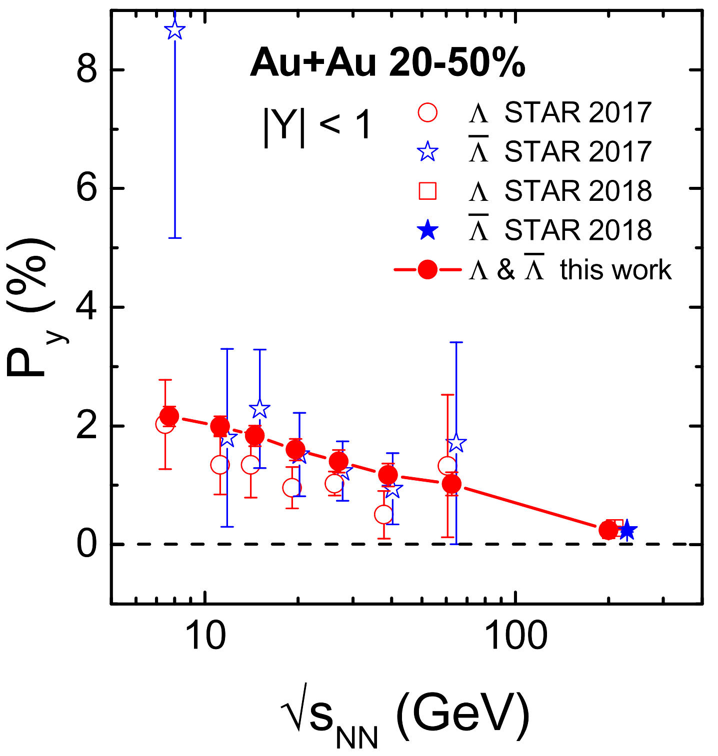
Substituting the theoretically calculated thermal vorticity shown in Fig. 4 into Eqs. (21)-(23), we can obtain the component of the spin polarization. This reflects the global angular momentum of the collision system and is called the global spin polarization; see Fig. 11 for global spin polarization of and (in short, “ polarization”) Wei et al. 2019. In addition, the experimental data from the STAR Collaboration are also shown Adamczyk et al. 2017; Adam et al. 2018. We find that the theoretical results fit the data very well. We note that similar calculations were performed by using either transport or hydrodynamic models, and good matches with the experimental data were seen in all those calculations Karpenko and Becattini 2017; Xie et al. 2017; Li et al. 2017; Sun and Ko 2017; Shi et al. 2019b; Csernai et al. 2019; Wei et al. 2019; Xie et al. 2019; Ivanov et al. 2019. From Fig. 11, we can see two special features of the global polarization. One is that the global polarization (as well as the vorticity) is smaller for larger . This contradicts our intuition because the total angular momentum of the system should be greater for larger . This is a relativistic effect: with increasing collision energy, the created hot matter at mid-rapidity behaves increasingly boost-invariant along the beam direction, thus supporting gradually less vorticity at mid-rapidity Deng and Huang 2016; Jiang et al. 2016. However, for a very-low-energy collision, the system may be nonrelativistic and the initial vorticity, which well reflects the angular momentum retained in the mid-rapidity region, would increase with Deng et al. 2020. The other feature is as follows: despite a big error bar, the experimental data show that spin polarization is less than spin polarization. Some possibilities for this difference have been recently discussed Han and Xu 2018; Guo et al. 2019a; Guo et al. 2019b; Csernai et al. 2019. For example, as the Zeeman coupling between the magnetic field and spin depends on the magnetic moment of the particle, , which has a positive magnetic moment, is more easily polarized than , which has a negative magnetic moment.
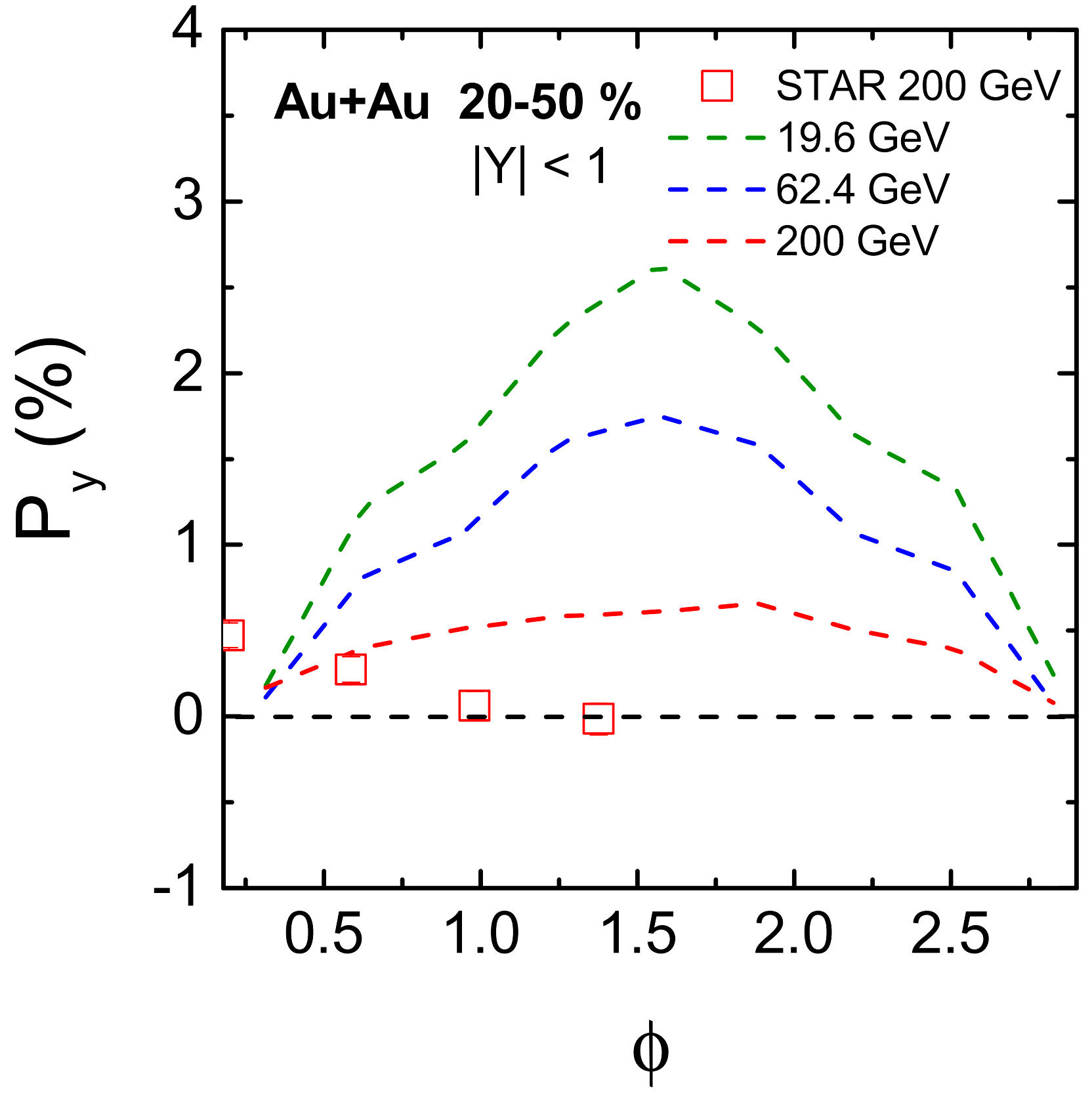
Recently, the STAR Collaboration published their measurements of differential spin polarization, namely, the dependence of polarization on the kinematic variables such as the azimuthal angle and transverse momentum Adam et al. 2018; Adam et al. 2019c. In describing the differential spin polarization, the theoretical calculations thus far have been unsatisfactory. In particular, the calculations based on hydrodynamic and transport models show that (: azimuthal angle) at mid-rapidity increases when grows from to . However, the experimental data show the opposite; see Fig. 12 Wei et al. 2019. Similarly, for noncentral collisions, a nonzero longitudinal polarization is observed in experiments (where this polarization vanishes when integrated over all the angles ), indicating a dependence that is also qualitatively opposite to the theoretical calculations of thermal vorticity Becattini and Karpenko 2018; Xia et al. 2018; Wei et al. 2019; see Fig. 13. Expressed in formula as
| (24) |
the second-order harmonic coefficient (and ) has the opposite sign in current theoretical calculations and in experimental data (i.e., while ). This is a huge puzzle. We call it the “spin sign problem.¡¯¡¯ To resolve the spin sign problem, some important issues should be carefully re-examined. (1) Approximately of the measured and are from decays of other higher-lying hadrons. During these decays, it is possible (e.g., in ) that the spin-polarization direction of the daughter is flipped as compared with the parent particle. Recent studies have shown that these decay contributions, despite suppressing of the primary polarization, are insufficient to resolve the spin sign problem Xia et al. 2019; Becattini et al. 2019. (2) Possible initial local spin polarization or an initial flow profile that can lead to finite local vorticity have not been encoded in hydrodynamic and transport models. It is a crucial future task to perform a numerical test of these possible initial conditions. (3) The formula (21) is derived based on the assumption that both momentum and spin degrees of freedom are at global equilibrium. This is a strong assumption that may not conform with a realistic case in heavy-ion collisions. Apart from global equilibrium, spin polarization is no longer enslaved to thermal vorticity and should be treated as an independent dynamical variable. Developing new theoretical framework that is beyond the global equilibrium assumption is very urgent. These frameworks, in both hydrodynamic and kinetic setups, have considerably progressed recently. We will discuss the hydrodynamic and kinetic frameworks with spin as a dynamical variable in the following sections. (4) Understanding the polarization dynamics is important. Recent studies include Refs. Li and Yee 2018; Zhang et al. 2019; Kapusta et al. 2020; Ayala et al. 2020a; Ayala et al. 2020b. (5) Other issues that may influence the polarization should also be explored (e.g., hadronic mean-fields Csernai et al. 2019, chiral-anomaly-induced effects Sun and Ko 2019; Liu et al. 2019a, other possible spin chemical potentials Florkowski et al. 2019a; Wu et al. 2019; Xie et al. 2020, and the gluonic contribution). Testing complementary observables to measure the vorticity is also helpful (e.g., the - and -spin alignment Liang and Wang 2005b, the CVEs and CVW, and the recently proposed vorticity-dependent hadron yields Taya et al. 2020).
To conclude this section, we explain how the special pattern of the thermal vorticity shown in Fig. 13 emerges. Although in Sec. II we discussed the fact that the global angular momentum of the collision system is the cause of vorticity, it is not the only cause. There are many other sources of vorticity. One important source is the inhomogeneous expansion of the fireball. Because in the non-central collisions, the fireball is almond shaped, the gradient of pressure would more strongly drive the fireball expanse along the reaction plane, and this is why we observe positive elliptic flow . In this type of expansion, we can easily imagine that a vortical structure with four vortices in four quadrants of the - plane () would appear. Of course, the temperature is also inhomogeneous and its gradient also contributes to the thermal vorticity, which together with the gradient of the velocity field gives the pattern shown in Fig. 13.

VI Spin hydrodynamics
Many attempts have been made to solve the spin sign problem. However, thus far, no satisfactory solution has been found. From a theoretical point of view, a key step forward would be to develop new theoretical frameworks to describe the spin polarization beyond the global equilibrium assumption. One promising framework is hydrodynamics, which very effectively describes the bulk evolution of the fireball in heavy-ion collisions, with the dynamical spin degree of freedom encoded. This type of framework is the spin hydrodynamics in which the spin polarization density (or equivalently the spin chemical potential) is treated on the same level as temperature and flow velocity Florkowski et al. 2018b; Montenegro and Torrieri 2019; Florkowski et al. 2019b; Hattori et al. 2019a; Bhadury et al. 2020.
In first-order spin hydrodynamics, the energy-momentum and spin current tensors are given by
| (25) |
in which we have chosen the Landau–Lifshitz frame. Here, is the energy density, is the pressure, are shear and bulk viscous tensors, and are related to the spin degree of freedom and represent the strength of the torque on the temporal and spacial components of the spin current tensor. The constitutive relations are given as Hattori et al. 2019a
| (26) | |||
| (27) | |||
| (28) | |||
| (29) |
where is anti-symmetrization in indices ; is traceless symmetrization in indices ; is the expansion rate; is the spatial projection; is the co-moving time derivative; is the spatial derivative; is called the spin chemical potential in which . Here, , and are the transport coefficients, which must be semi-positive. We call them the shear viscosity, bulk viscosity, boost heat conductivity, and rotational viscosity, respectively Hattori et al. 2019a. A recent attempt at calculating the spin-related transport coefficient is given in Ref. Li and Yee 2019. The hydrodynamic equations are as follows:
| (30) | |||
| (31) |
To make the aforementioned equation close, we also need the equation of state, which links .
In practical use, the aforementioned first-order theory has non-physical modes at the ultraviolet region, which violates the relativistic causality and leads to numerical instability. This problem stems from the constitutive relations Eqs. (26)-(29) that represent simple proportionality between the responses of the fluid (i.e., LHSs) and the corresponding forces (i.e., RHSs). The simplest means of overcoming this drawback of first-order hydrodynamics is to amend Eqs. (26)-(29) to the Israel-Stewart form:
| (32) | |||
| (33) | |||
| (34) | |||
| (35) |
where means taking the components transverse to (e.g., ). In these equations, , and are treated as dynamical variables as well. Therefore, we also need additional initial conditions for them in practical use. They relax to the constitutive relations Eqs. (26)-(29) after a time scale much greater than the relaxation times , and . In this manner, we obtain a set of closed, numerically stable, hydrodynamic equations. The next step is to develop a numerical application to heavy-ion collisions; Hopefully, it can provide us with valuable insights into the spin sign problem.
VII Chiral and spin kinetic theories
In addition to hydrodynamics, kinetic theory is another commonly used method to study many-body systems in and out of equilibrium. Let us start with a short review of classical kinetic theory.
VII.1 Classical kinetic theory
Classically, kinetic theory is built based on a single particle distribution function, which is a scalar function defined in the phase space. The physical meaning of the single particle distribution, which we denote as , is the number of particles with a specific space location and momentum at time . The kinetic equation determines the time evolution of and was first proposed by Boltzmann in the following form:
| (36) |
where is the single particle velocity with particle mass , is the external force, and is the collision term, which is a functional of . The LHS of the aforementioned equation is the evolution of due to streaming in the phase space with the existence of the external force field. In other words, the particle at the phase space point moves with the velocity and the momentum-space velocity at time , which leads to the change in the distribution function . RHS denotes the collision effects among particles that can change the momentum (and possibly also the location) of the particle under study.
Considering the special relativity, we can generalize Eq. (36) into a relativistic kinetic equation De Groot et al. 1980. We adopt the Minkowski metric and the convention , and we define the eight-dimensional phase space coordinates as , where and , with being the energy coordinate. Particles satisfy the following on-shell condition . Defining the distribution function in the eight-dimensional phase space, we write the relativistic kinetic equation in the form
| (37) |
where is the single particle four velocity and is the four external force. The external force is called mechanical if it satisfies the condition , which leads to the condition according to the on-shell condition. Furthermore, we obtain . In the following discussion, we always assume to be mechanical. Substituting the solution of into Eq. (37) and using the chain rule
| (38) |
we reproduce the form of the LHS of Eq. (36) in the nonrelativistic kinetic representation.
The relations between physical quantities and the distribution function are readily obtained. The most elementary quantity is the particle density , which is expressed as . The particle three current is defined as . Combining the particle density and the three current, we obtain the four current as . In relativistic kinetic theory, the covariant four current can be written concisely as follows:
| (39) |
where the delta function ensures that the particles are on-shell. Next, we consider the energy-momentum tensor. Classically, the energy-momentum tensor can be explained as the covariant current of the four momentum and thus reads as
| (40) |
The energy-momentum tensor is symmetric because the four velocity is proportional to the momentum . The entropy density is defined as . Similarly, we define the covariant entropy current as
| (41) |
The entropy current satisfies the second law of thermodynamics (the Boltzmann H-theorem) , where the equality holds in the global equilibrium state.
VII.2 Wigner function in non-relativistic physics
When quantum mechanics is in action, the aforementioned kinetic theory must be modified. Quantum kinetic theory can be built based on the Wigner function method Bonitz 1998. The Wigner function is the quantum correspondence of the classical distribution function first proposed by Wigner in 1932. In quantum mechanics, the properties of a particle are described by the wave function . The dynamics of a non-relativistic particle is governed by the Schrödinger equation:
| (42) |
where is the external potential. After the second quantization, we define the Wigner function as
| (43) |
where , and refers to the ensemble average. Note that the Wigner function is real.
The dynamics of the Wigner function is derived from the Schrödinger equation (42). Define . We obtain
| (44) | |||||
where we have integrated by parts. Next, we suppose that the gradient of the potential is small so that we can make a gradient expansion. At the first order in , we have and thus Eq. (44) reduces to
| (45) |
We thus identify the Wigner function as the single particle distribution function and identify the external force . Thus, Eq. (45) is reduced to the classical kinetic equation (36) without the collision term. To obtain the collision term, we must start with an interacting theory rather than the Schrödinger equation. The Wigner function method is particularly useful in performing the semiclassical approach to the quantum kinetic theory of spinful particles. Therefore, we next discuss quantum kinetic theory as related to spin- particles.
VII.3 Kinetic theory for Spin- fermions
With the aforementioned warmup preparation, we now consider the Dirac fermions. We not only introduce the Wigner function for the spinor field Vasak et al. 1987 but also review the derivation of the kinetic theory available in curved spacetime and the external EM field for Dirac fermions Winter 1985; Calzetta et al. 1988; Fonarev 1994; Liu et al. 2019b; Liu et al. 2020. In quantum field theory in Minkowski spacetime, the spin- particle is described by the Dirac field , which is in general a four-component spinor field. We must establish a local flat frame to introduce the spinor into curved spacetime. This is naturally done by using the vierbein field , which can be considered as a coordinate transformation between the general coordinate of the spacetime manifold and the local flat Minkowski coordinate. We use (un)hatted Greek indices to denote local flat (curved) spacetime coordinates. In addition, denotes the covariant derivative with respect to the diffeomorphism and denotes the curved spacetime metric. The Levi-Civita symbol is with and . The dynamics of the Dirac field obey the Dirac equation
| (46) |
where the Dirac matrices satisfy , with the spin connection and the spin matrix , is the gauge potential, and .
Next, we establish the phase space in curved spacetime to introduce the Wigner function and the kinetic theory. We use the cotangent vector to denote the momentum in curved spacetime with as its conjugate variable. Thus, the momentum space is the cotangent space of the spacetime manifold at a given point. The local inner product of the momentum space and the spacetime manifold constitute the phase space, which is the cotangent bundle Nakahara 2003. constitutes the tangent space at a given point of the spacetime manifold, and the tangent bundle is locally the inner product of the tangent space and the spacetime manifold. We introduce the horizontal lifts of the covariant derivative in the cotangent bundle and the tangent bundle . With the horizontal lift, we can verify that .
The covariant Wigner operator under the U(1) gauge, local Lorentz transformation, and diffeomorphism are defined as Liu et al. 2019b
| (47) |
with and , where also contains the gauge field when acting on a charged spinor: . The Wigner function is defined by replacing the operator with the ensemble average in Eq. (47). The dynamics of the Wigner function with full quantum corrections are derived with the help of the Dirac equation (46), which can be solved by the expansion method with respect to with the power counting scheme and Liu et al. 2019b. Up to , the dynamic equation reads as Liu et al. 2019b
| (48) |
with
| (49) |
where is the Ricci tensor. We find that the spacetime curvature comes at at least. The Wigner function for the Dirac field is a matrix, which is different from the scalar case discussed in the previous subsection. Thus, the relation between the Wigner function and the semiclassical distribution function is less obvious in the spinor case. Equation (48) holds 16 scalar equations if we separate its matrix components, which can be decomposed into hermitian and antihermitian parts further.
Thus, we decompose the Wigner function based on Clifford algebra: , where and all the Clifford coefficients are real. Furthermore, Eq. (48) can be decomposed into dynamic equations for the Clifford coefficients. The Clifford coefficients are not independent. We choose the independent variables as and . The physical meanings of and are the vector current density and the axial current density in the phase space, respectively, where the latter is also related to the canonical spin current density in phase space. Therefore, the vector current, axial current, and canonical spin current are respectively given by , , and with . In the limit , the vector is proportional to the momentum , which is in accordance with Eq. (39). However, the axial vector has different forms in the massless and massive cases because spin is parallel (or anti-parallel) to the momentum for a massless particle and is perpendicular to the momentum for a massive particle. Although spin is not an independent variable in the massless case, it induces a Berry curvature, which leads to nontrivial topological effects and results in the chiral kinetic theory. While in the massive case, spin becomes an independent variable, which induces two new degrees of freedom (i.e., the orientation of the spin vector). The complete set of kinetic equations in the massive case is thus composed of four equations. We call this theory the spin kinetic theory. Let us discuss the chiral and spin kinetic theories separately in the following sections.
VII.3.1 Chiral kinetic theory
For massless fermions, in the classical limit, not only but also is parallel to the momentum, and up to , they read as
| (50) | |||||
where and are two scalar coefficients, is the spin tensor for chiral fermions with being a unit time-like frame vector, and the delta function imposes the mass-shell condition at a classical limit. Comparing the vector and axial currents for massless fermions with Eq. (39), we find that the two scalar functions and represent the semiclassical vector distribution function and axial distribution function, respectively. The second term in Eq. (50) is called the side-jump term, which ensures the total angular momentum to be conserved during collisions of two massless fermions Chen et al. 2014, whereas the last term comes from the interaction between the spin and external EM field.
We define the right- and left-hand distribution functions as . The kinetic equations for and are derived as Liu et al. 2019b
| (51) | |||||
where the mass-shell condition is corrected by the interaction between spin and the external EM field at . The flat spacetime version of the aforementioned chiral kinetic equation has been under intensive investigations recently Son and Yamamoto 2012; Stephanov and Yin 2012; Gao et al. 2012; Son and Yamamoto 2013; Chen et al. 2013; Chen et al. 2014; Chen et al. 2015; Huang 2016b; Hidaka et al. 2017; Mueller and Venugopalan 2017; Carignano et al. 2018; Huang et al. 2018; Huang and Sadofyev 2019; Lin and Shukla 2019; Lin and Yang 2020; Gao et al. 2020, which can be written in the following form (for right-hand particles only) after being integrated out:
| (52) | |||||
where we have chosen , as the particle energy and as the effective velocity. We find that a phase space correction factor exists, where is the Berry curvature. The dispersion relation is also corrected by the Berry curvature at . The three components for the right-hand particles take the form
| (53) | |||||
Similarly, the kinetic equation and current for left-hand particles can be readily derived.
The kinetic theory in curved spacetime can be used to study the rotating frame. We consider the frame as rotating with the angular velocity in the inertial frame, and we choose the frame vector . The kinetic equation reads as Liu et al. 2019b
| (54) |
where and . We find the correspondence between the rotation velocity and magnetic field in (thus in ) is , whereas other places is . The current is
| (55) |
The equilibrium state can be derived from the kinetic equation (51). We suppose the local equilibrium distribution functions depend on a linear combination of the collisional conserved quantities: the particle number, energy and momentum, and angular momentum. Therefore, we have with , where the coefficients ’s, and depend only on ; is time-like; and is supposed to be the Fermi–Dirac distribution function. The global equilibrium condition is derived as Liu et al. 2019b
| (56) |
where is an arbitrary function that arises as a result of the conformal invariance in the massless case. We define the four velocity of the fluid as with being the temperature, and the chemical potential . Substituting the global equilibrium condition into Eqs. (53) and (55) and considering also the current of left-hand particles, we derive the CME and CSE as
| (57) |
where and , and the CVEs
| (58) |
We should note that the results for the CME and CVE currents are independent of the choice of the frame vector .
VII.3.2 Spin kinetic theory
For massive fermions, the particle spin is perpendicular to its momentum up to . The expressions of the vector and the axial vector are as follows:
| (59) | |||||
| (60) |
where and are two scalar functions and is the unit spacelike spin vector that is perpendicular to momentum . We define , which satisfy the following relation:
| (61) |
where is the spin tensor for massive fermions and is the spin projection operator Kaku 1993. Thus, the physical meanings of are the semiclassical distribution functions that describe the spin-up and spin-down states with respect to . The kinetic equations for are derived as Liu et al. 2020
| (62) | |||||
The evolution equation for the spin-direction vector is given by Liu et al. 2020
| (63) | |||||
We emphasize that the third term on the right-hand side is actually order. From the kinetic equations, we can extract the Mathisson–Papapetrou–Dixon equations as
| (64) | |||||
| (65) |
where is the proper time along the trajectory of the particle and . The previous two equations describe the spin dynamics for a single particle in curved spacetime and the external EM field.
We can derive the equilibrium state for massive fermions using the same method as in the massless case. Supposing with and substituting it into Eq. (62), we verify that the following conditions make Eq. (62) hold:
| (66) |
where we use De Groot et al. 1980. Furthermore, we find that the following solutions of and satisfy the spin evolution equation (63) Liu et al. 2020:
| (67) |
where with . Thus, the particle spin is polarized along the thermal vorticity at global equilibrium. The spin polarization per particle in the phase space is defined by . Substituting the global equilibrium conditions (66) and (67), we obtain
| (68) | |||||
which, after integrating over to , yields formula (21) for and with the contribution from the EM field added. (Note that in Eq. (21), the approximation is used as for hyperon, for example, is large.) More details on collisionless spin kinetic theory in flat space are provided in Refs. Gao and Liang 2019; Weickgenannt et al. 2019; Hattori et al. 2019b; Wang et al. 2019. Discussions on the collision terms in CKT and SKT are found in Refs. Carignano et al. 2019; Li and Yee 2019; Chen et al. 2015; Hidaka et al. 2017; Yang et al. 2020; Yamamoto and Yang 2020.
VIII Summary
We discussed some intriguing properties of the strong EM fields and vorticity in heavy-ion collisions. We provided a heuristic introduction to the anomalous chiral transport phenomena and spin polarization in heavy-ion collisions. We briefly reviewed the recent progress in both theory and experiments toward understanding these novel quantum phenomena in heavy-ion collisions. The ACTs could be used to detect the nontrivial topological structure of the QCD gauge sector and the possible P and CP violations of strong interaction in a high-temperature environment. The spin polarization of hadrons provides us a probe to the (local) rotating properties and to the spin dynamics of the quark-gluon matter. This opens a door to a new era of subatomic spintronics.
Some challenges remain. Noticeably, the experimental observables for the ACTs (e.g., the CME) contain strong background contributions, which call for more efforts and new ideas from both the theoretical and experimental sides to be resolved. The experimental data for the azimuthal-angle dependence of spin polarization show a qualitatively opposite trend as compared to the thermal vorticity based on theoretical calculations, which gives rise to a spin sign problem. It is promising that new theoretical frameworks with spin as an independent dynamical variable may provide important insight into the spin sign problem. Presently, two of these frameworks, namely, spin hydrodynamics and spin kinetic theory, are progressing rapidly, and hopefully in the near future, the numerical simulations based on them could be achieved.
Acknowledgments— We thank J. Bloczynski, W. T. Deng, X. G. Deng, L. L. Gao, K. Hattori, M. Hongo, H. Z. Huang, P. Huovinen, H. Li, Y. Jiang, J. Liao, D. E. Kharzeev, G. L. Ma, Y. G. Ma, K. Mameda, M. Matsuo, L. G. Pang, A. V. Sadofyev, H. Taya, G. Wang, Q. Wang, X. N. Wang, D. X. Wei, H. Z. Wu, X. L. Xia, Y. Yin, S. Zhang, and X. Zhang for collaboration on the topics covered in this article. This work is supported by NSFC under Grant Nos. 11535012 and 11675041.
References
- Wang (2016) X.-N. Wang, ed., Quark Gluon Plasma 5 (Singapore: World Scientific Publishing, 2016).
- Kharzeev et al. (2016) D. E. Kharzeev, J. Liao, S. A. Voloshin, and G. Wang, Prog. Part. Nucl. Phys. 88, 1 (2016), arXiv:1511.04050 [hep-ph] .
- Huang (2016a) X.-G. Huang, Rept. Prog. Phys. 79, 076302 (2016a), arXiv:1509.04073 [nucl-th] .
- Hattori and Huang (2017) K. Hattori and X.-G. Huang, Nucl. Sci. Tech. 28, 26 (2017), arXiv:1609.00747 [nucl-th] .
- Koch et al. (2017) V. Koch, S. Schlichting, V. Skokov, P. Sorensen, J. Thomas, S. Voloshin, G. Wang, and H.-U. Yee, Chin. Phys. C41, 072001 (2017), arXiv:1608.00982 [nucl-th] .
- Zhao and Wang (2019) J. Zhao and F. Wang, Prog. Part. Nucl. Phys. 107, 200 (2019), arXiv:1906.11413 [nucl-ex] .
- Li and Wang (2020) W. Li and G. Wang, (2020), arXiv:2002.10397 [nucl-ex] .
- Becattini and Lisa (2020) F. Becattini and M. Lisa, (2020), 10.1146/annurev-nucl-021920-095245, arXiv:2003.03640 [nucl-ex] .
- Huang (2020) X.-G. Huang, (2020), arXiv:2002.07549 [nucl-th] .
- Kaspi and Beloborodov (2017) V. M. Kaspi and A. Beloborodov, Ann. Rev. Astron. Astrophys. 55, 261 (2017), arXiv:1703.00068 [astro-ph.HE] .
- Skokov et al. (2009) V. Skokov, A. Yu. Illarionov, and V. Toneev, Int. J. Mod. Phys. A24, 5925 (2009), arXiv:0907.1396 [nucl-th] .
- Voronyuk et al. (2011) V. Voronyuk, V. D. Toneev, W. Cassing, E. L. Bratkovskaya, V. P. Konchakovski, and S. A. Voloshin, Phys. Rev. C83, 054911 (2011), arXiv:1103.4239 [nucl-th] .
- Bzdak and Skokov (2012) A. Bzdak and V. Skokov, Phys. Lett. B710, 171 (2012), arXiv:1111.1949 [hep-ph] .
- Ou and Li (2011) L. Ou and B.-A. Li, Phys. Rev. C84, 064605 (2011), arXiv:1107.3192 [nucl-th] .
- Deng and Huang (2012) W.-T. Deng and X.-G. Huang, Phys. Rev. C85, 044907 (2012), arXiv:1201.5108 [nucl-th] .
- Bloczynski et al. (2013) J. Bloczynski, X.-G. Huang, X. Zhang, and J. Liao, Phys. Lett. B718, 1529 (2013), arXiv:1209.6594 [nucl-th] .
- Bloczynski et al. (2015) J. Bloczynski, X.-G. Huang, X. Zhang, and J. Liao, Nucl. Phys. A939, 85 (2015), arXiv:1311.5451 [nucl-th] .
- Deng and Huang (2015) W.-T. Deng and X.-G. Huang, Phys. Lett. B742, 296 (2015), arXiv:1411.2733 [nucl-th] .
- Zhong et al. (2014) Y. Zhong, C.-B. Yang, X. Cai, and S.-Q. Feng, Adv. High Energy Phys. 2014, 193039 (2014), arXiv:1408.5694 [hep-ph] .
- Zhong et al. (2015) Y. Zhong, C.-B. Yang, X. Cai, and S.-Q. Feng, Chin. Phys. C39, 104105 (2015), arXiv:1410.6349 [hep-ph] .
- Huang et al. (2016) X.-G. Huang, Y. Yin, and J. Liao, Nucl. Phys. A956, 661 (2016), arXiv:1512.06602 [nucl-th] .
- Deng et al. (2016) W.-T. Deng, X.-G. Huang, G.-L. Ma, and G. Wang, Phys. Rev. C94, 041901 (2016), arXiv:1607.04697 [nucl-th] .
- Huang et al. (2017) X.-G. Huang, W.-T. Deng, G.-L. Ma, and G. Wang, Nucl. Phys. A967, 736 (2017), arXiv:1704.04382 [nucl-th] .
- Zhao et al. (2018) X.-L. Zhao, Y.-G. Ma, and G.-L. Ma, Phys. Rev. C97, 024910 (2018), arXiv:1709.05962 [hep-ph] .
- Deng and Ma (2017) X.-G. Deng and Y.-G. Ma, Nucl. Sci. Tech. 28, 182 (2017).
- Cheng et al. (2019) Y.-L. Cheng, S. Zhang, Y.-G. Ma, J.-H. Chen, and C. Zhong, Phys. Rev. C99, 054906 (2019), arXiv:1909.03160 [nucl-th] .
- Becattini et al. (2015) F. Becattini, G. Inghirami, V. Rolando, A. Beraudo, L. Del Zanna, A. De Pace, M. Nardi, G. Pagliara, and V. Chandra, Eur. Phys. J. C75, 406 (2015), [Erratum: Eur. Phys. J.C78,no.5,354(2018)], arXiv:1501.04468 [nucl-th] .
- Deng and Huang (2016) W.-T. Deng and X.-G. Huang, Phys. Rev. C93, 064907 (2016), arXiv:1603.06117 [nucl-th] .
- Becattini (2012) F. Becattini, Phys. Rev. Lett. 108, 244502 (2012), arXiv:1201.5278 [gr-qc] .
- Becattini et al. (2013) F. Becattini, V. Chandra, L. Del Zanna, and E. Grossi, Annals Phys. 338, 32 (2013), arXiv:1303.3431 [nucl-th] .
- Adamczyk et al. (2017) L. Adamczyk et al. (STAR), Nature 548, 62 (2017), arXiv:1701.06657 [nucl-ex] .
- Wei et al. (2019) D.-X. Wei, W.-T. Deng, and X.-G. Huang, Phys. Rev. C99, 014905 (2019), arXiv:1810.00151 [nucl-th] .
- Jiang et al. (2016) Y. Jiang, Z.-W. Lin, and J. Liao, Phys. Rev. C94, 044910 (2016), [Erratum: Phys. Rev.C95,no.4,049904(2017)], arXiv:1602.06580 [hep-ph] .
- Teryaev and Usubov (2015) O. Teryaev and R. Usubov, Phys. Rev. C92, 014906 (2015).
- Xie et al. (2016) Y. L. Xie, M. Bleicher, H. St?cker, D. J. Wang, and L. P. Csernai, Phys. Rev. C94, 054907 (2016), arXiv:1610.08678 [nucl-th] .
- Ivanov and Soldatov (2017) Yu. B. Ivanov and A. A. Soldatov, Phys. Rev. C95, 054915 (2017), arXiv:1701.01319 [nucl-th] .
- Kolomeitsev et al. (2018) E. E. Kolomeitsev, V. D. Toneev, and V. Voronyuk, Phys. Rev. C97, 064902 (2018), arXiv:1801.07610 [nucl-th] .
- Deng et al. (2020) X.-G. Deng, X.-G. Huang, Y.-G. Ma, and S. Zhang, (2020), arXiv:2001.01371 [nucl-th] .
- Landsteiner (2016) K. Landsteiner, Acta Phys. Polon. B47, 2617 (2016), arXiv:1610.04413 [hep-th] .
- Huang (2018) X.-G. Huang, EPJ Web Conf. 172, 01003 (2018), arXiv:1802.00172 [nucl-th] .
- Adler (1969) S. L. Adler, Phys. Rev. 177, 2426 (1969), [,241(1969)].
- Bell and Jackiw (1969) J. S. Bell and R. Jackiw, Nuovo Cim. A60, 47 (1969).
- Kharzeev et al. (2008) D. E. Kharzeev, L. D. McLerran, and H. J. Warringa, Nucl. Phys. A803, 227 (2008), arXiv:0711.0950 [hep-ph] .
- Fukushima et al. (2008) K. Fukushima, D. E. Kharzeev, and H. J. Warringa, Phys. Rev. D78, 074033 (2008), arXiv:0808.3382 [hep-ph] .
- Son and Zhitnitsky (2004) D. T. Son and A. R. Zhitnitsky, Phys. Rev. D70, 074018 (2004), arXiv:hep-ph/0405216 [hep-ph] .
- Metlitski and Zhitnitsky (2005) M. A. Metlitski and A. R. Zhitnitsky, Phys. Rev. D72, 045011 (2005), arXiv:hep-ph/0505072 [hep-ph] .
- Vilenkin (1979) A. Vilenkin, Phys. Rev. D20, 1807 (1979).
- Erdmenger et al. (2009) J. Erdmenger, M. Haack, M. Kaminski, and A. Yarom, JHEP 01, 055 (2009), arXiv:0809.2488 [hep-th] .
- Banerjee et al. (2011) N. Banerjee, J. Bhattacharya, S. Bhattacharyya, S. Dutta, R. Loganayagam, and P. Surowka, JHEP 01, 094 (2011), arXiv:0809.2596 [hep-th] .
- Son and Surowka (2009) D. T. Son and P. Surowka, Phys. Rev. Lett. 103, 191601 (2009), arXiv:0906.5044 [hep-th] .
- Landsteiner et al. (2011) K. Landsteiner, E. Megias, and F. Pena-Benitez, Phys. Rev. Lett. 107, 021601 (2011), arXiv:1103.5006 [hep-ph] .
- Glorioso et al. (2019) P. Glorioso, H. Liu, and S. Rajagopal, JHEP 01, 043 (2019), arXiv:1710.03768 [hep-th] .
- Hirono et al. (2014a) Y. Hirono, M. Hongo, and T. Hirano, Phys. Rev. C90, 021903 (2014a), arXiv:1211.1114 [nucl-th] .
- Voronyuk et al. (2014) V. Voronyuk, V. D. Toneev, S. A. Voloshin, and W. Cassing, Phys. Rev. C90, 064903 (2014), arXiv:1410.1402 [nucl-th] .
- Huang and Liao (2013) X.-G. Huang and J. Liao, Phys. Rev. Lett. 110, 232302 (2013), arXiv:1303.7192 [nucl-th] .
- Pu et al. (2014) S. Pu, S.-Y. Wu, and D.-L. Yang, Phys. Rev. D89, 085024 (2014), arXiv:1401.6972 [hep-th] .
- Bu et al. (2018) Y. Bu, R.-G. Cai, Q. Yang, and Y.-L. Zhang, JHEP 09, 083 (2018), arXiv:1803.08389 [hep-th] .
- Zyuzin (2018) V. A. Zyuzin, Phys. Rev. B98, 165205 (2018), arXiv:1803.00723 [cond-mat.mes-hall] .
- Jiang et al. (2015a) Y. Jiang, X.-G. Huang, and J. Liao, Phys. Rev. D91, 045001 (2015a), arXiv:1409.6395 [nucl-th] .
- Ding et al. (2016) H.-T. Ding, O. Kaczmarek, and F. Meyer, Phys. Rev. D94, 034504 (2016), arXiv:1604.06712 [hep-lat] .
- Kharzeev and Yee (2011) D. E. Kharzeev and H.-U. Yee, Phys. Rev. D83, 085007 (2011), arXiv:1012.6026 [hep-th] .
- Jiang et al. (2015b) Y. Jiang, X.-G. Huang, and J. Liao, Phys. Rev. D92, 071501 (2015b), arXiv:1504.03201 [hep-ph] .
- Kharzeev et al. (1998) D. Kharzeev, R. D. Pisarski, and M. H. G. Tytgat, Phys. Rev. Lett. 81, 512 (1998), arXiv:hep-ph/9804221 [hep-ph] .
- Kharzeev et al. (2002) D. Kharzeev, A. Krasnitz, and R. Venugopalan, Phys. Lett. B545, 298 (2002), arXiv:hep-ph/0109253 [hep-ph] .
- Kharzeev (2006) D. Kharzeev, Phys. Lett. B633, 260 (2006), arXiv:hep-ph/0406125 [hep-ph] .
- Voloshin (2004a) S. A. Voloshin, Phys. Rev. C70, 057901 (2004a), arXiv:hep-ph/0406311 [hep-ph] .
- Abelev et al. (2009) B. I. Abelev et al. (STAR), Phys. Rev. Lett. 103, 251601 (2009), arXiv:0909.1739 [nucl-ex] .
- Abelev et al. (2010) B. I. Abelev et al. (STAR), Phys. Rev. C81, 054908 (2010), arXiv:0909.1717 [nucl-ex] .
- Abelev et al. (2013) B. Abelev et al. (ALICE), Phys. Rev. Lett. 110, 012301 (2013), arXiv:1207.0900 [nucl-ex] .
- Acharya et al. (2018) S. Acharya et al. (ALICE), Phys. Lett. B777, 151 (2018), arXiv:1709.04723 [nucl-ex] .
- Khachatryan et al. (2017) V. Khachatryan et al. (CMS), Phys. Rev. Lett. 118, 122301 (2017), arXiv:1610.00263 [nucl-ex] .
- Sirunyan et al. (2018) A. M. Sirunyan et al. (CMS), Phys. Rev. C97, 044912 (2018), arXiv:1708.01602 [nucl-ex] .
- Adamczyk et al. (2014) L. Adamczyk et al. (STAR), Phys. Rev. Lett. 113, 052302 (2014), arXiv:1404.1433 [nucl-ex] .
- Pratt et al. (2011) S. Pratt, S. Schlichting, and S. Gavin, Phys. Rev. C84, 024909 (2011), arXiv:1011.6053 [nucl-th] .
- Bzdak et al. (2011) A. Bzdak, V. Koch, and J. Liao, Phys. Rev. C83, 014905 (2011), arXiv:1008.4919 [nucl-th] .
- Schlichting and Pratt (2011) S. Schlichting and S. Pratt, Phys. Rev. C83, 014913 (2011), arXiv:1009.4283 [nucl-th] .
- Wang (2010) F. Wang, Phys. Rev. C81, 064902 (2010), arXiv:0911.1482 [nucl-ex] .
- Adam et al. (2019a) J. Adam et al. (STAR), Phys. Lett. B798, 134975 (2019a), arXiv:1906.03373 [nucl-ex] .
- Voloshin (2010) S. A. Voloshin, Phys. Rev. Lett. 105, 172301 (2010), arXiv:1006.1020 [nucl-th] .
- Xu et al. (2018a) H.-J. Xu, X. Wang, H. Li, J. Zhao, Z.-W. Lin, C. Shen, and F. Wang, Phys. Rev. Lett. 121, 022301 (2018a), arXiv:1710.03086 [nucl-th] .
- Li et al. (2018) H. Li, H.-j. Xu, J. Zhao, Z.-W. Lin, H. Zhang, X. Wang, C. Shen, and F. Wang, Phys. Rev. C98, 054907 (2018), arXiv:1808.06711 [nucl-th] .
- Sun and Ko (2018) Y. Sun and C. M. Ko, Phys. Rev. C98, 014911 (2018), arXiv:1803.06043 [nucl-th] .
- Magdy et al. (2018a) N. Magdy, S. Shi, J. Liao, P. Liu, and R. A. Lacey, Phys. Rev. C98, 061902 (2018a), arXiv:1803.02416 [nucl-ex] .
- Shi et al. (2019a) S. Shi, H. Zhang, D. Hou, and J. Liao, (2019a), arXiv:1910.14010 [nucl-th] .
- Adam et al. (2019b) J. Adam et al. (STAR), (2019b), arXiv:1911.00596 [nucl-ex] .
- Zhao et al. (2019) J. Zhao, H. Li, and F. Wang, Eur. Phys. J. C79, 168 (2019), arXiv:1705.05410 [nucl-ex] .
- Zhao (2019) J. Zhao (STAR), Proceedings, 27th International Conference on Ultrarelativistic Nucleus-Nucleus Collisions (Quark Matter 2018): Venice, Italy, May 14-19, 2018, Nucl. Phys. A982, 535 (2019), arXiv:1807.09925 [nucl-ex] .
- Xu et al. (2018b) H.-j. Xu, J. Zhao, X. Wang, H. Li, Z.-W. Lin, C. Shen, and F. Wang, Chin. Phys. C42, 084103 (2018b), arXiv:1710.07265 [nucl-th] .
- Tang (2019) A. H. Tang, (2019), arXiv:1903.04622 [nucl-ex] .
- Magdy et al. (2018b) N. Magdy, S. Shi, J. Liao, N. Ajitanand, and R. A. Lacey, Phys. Rev. C97, 061901 (2018b), arXiv:1710.01717 [physics.data-an] .
- Gorbar et al. (2011) E. V. Gorbar, V. A. Miransky, and I. A. Shovkovy, Phys. Rev. D83, 085003 (2011), arXiv:1101.4954 [hep-ph] .
- Burnier et al. (2011) Y. Burnier, D. E. Kharzeev, J. Liao, and H.-U. Yee, Phys. Rev. Lett. 107, 052303 (2011), arXiv:1103.1307 [hep-ph] .
- Burnier et al. (2012) Y. Burnier, D. E. Kharzeev, J. Liao, and H. U. Yee, (2012), arXiv:1208.2537 [hep-ph] .
- Taghavi and Wiedemann (2015) S. F. Taghavi and U. A. Wiedemann, Phys. Rev. C91, 024902 (2015), arXiv:1310.0193 [hep-ph] .
- Yee and Yin (2014) H.-U. Yee and Y. Yin, Phys. Rev. C89, 044909 (2014), arXiv:1311.2574 [nucl-th] .
- Hirono et al. (2014b) Y. Hirono, T. Hirano, and D. E. Kharzeev, (2014b), arXiv:1412.0311 [hep-ph] .
- Adamczyk et al. (2015) L. Adamczyk et al. (STAR), Phys. Rev. Lett. 114, 252302 (2015), arXiv:1504.02175 [nucl-ex] .
- Adam et al. (2016) J. Adam et al. (ALICE), Phys. Rev. C93, 044903 (2016), arXiv:1512.05739 [nucl-ex] .
- Sirunyan et al. (2019) A. M. Sirunyan et al. (CMS), Phys. Rev. C100, 064908 (2019), arXiv:1708.08901 [nucl-ex] .
- Stephanov and Yee (2013) M. Stephanov and H.-U. Yee, Phys. Rev. C88, 014908 (2013), arXiv:1304.6410 [nucl-th] .
- Dunlop et al. (2011) J. C. Dunlop, M. A. Lisa, and P. Sorensen, Phys. Rev. C84, 044914 (2011), arXiv:1107.3078 [hep-ph] .
- Xu et al. (2012) J. Xu, L.-W. Chen, C. M. Ko, and Z.-W. Lin, Phys. Rev. C85, 041901 (2012), arXiv:1201.3391 [nucl-th] .
- Ko et al. (2014) C. M. Ko, T. Song, F. Li, V. Greco, and S. Plumari, Nucl. Phys. A928, 234 (2014), arXiv:1211.5511 [nucl-th] .
- Bzdak and Bozek (2013) A. Bzdak and P. Bozek, Phys. Lett. B726, 239 (2013), arXiv:1303.1138 [nucl-th] .
- Hatta et al. (2016) Y. Hatta, A. Monnai, and B.-W. Xiao, Nucl. Phys. A947, 155 (2016), arXiv:1507.04690 [hep-ph] .
- Xu et al. (2020) H.-j. Xu, J. Zhao, Y. Feng, and F. Wang, Phys. Rev. C101, 014913 (2020), arXiv:1910.02896 [nucl-th] .
- Bzdak et al. (2019) A. Bzdak, S. Esumi, V. Koch, J. Liao, M. Stephanov, and N. Xu, (2019), arXiv:1906.00936 [nucl-th] .
- Ma and Huang (2015) G.-L. Ma and X.-G. Huang, Phys. Rev. C91, 054901 (2015), arXiv:1501.03903 [nucl-th] .
- Liang and Wang (2005a) Z.-T. Liang and X.-N. Wang, Phys. Rev. Lett. 94, 102301 (2005a), [Erratum: Phys. Rev. Lett.96,039901(2006)], arXiv:nucl-th/0410079 [nucl-th] .
- Voloshin (2004b) S. A. Voloshin, (2004b), arXiv:nucl-th/0410089 [nucl-th] .
- Gao et al. (2008) J.-H. Gao, S.-W. Chen, W.-t. Deng, Z.-T. Liang, Q. Wang, and X.-N. Wang, Phys. Rev. C77, 044902 (2008), arXiv:0710.2943 [nucl-th] .
- Huang et al. (2011) X.-G. Huang, P. Huovinen, and X.-N. Wang, Phys. Rev. C84, 054910 (2011), arXiv:1108.5649 [nucl-th] .
- Fang et al. (2016) R.-h. Fang, L.-g. Pang, Q. Wang, and X.-n. Wang, Phys. Rev. C94, 024904 (2016), arXiv:1604.04036 [nucl-th] .
- Florkowski et al. (2018a) W. Florkowski, B. Friman, A. Jaiswal, R. Ryblewski, and E. Speranza, Phys. Rev. D97, 116017 (2018a), arXiv:1712.07676 [nucl-th] .
- Liu et al. (2020) Y.-C. Liu, K. Mameda, and X.-G. Huang, (2020), arXiv:2002.03753 [hep-ph] .
- Adam et al. (2018) J. Adam et al. (STAR), Phys. Rev. C98, 014910 (2018), arXiv:1805.04400 [nucl-ex] .
- Karpenko and Becattini (2017) I. Karpenko and F. Becattini, Eur. Phys. J. C77, 213 (2017), arXiv:1610.04717 [nucl-th] .
- Xie et al. (2017) Y. Xie, D. Wang, and L. P. Csernai, Phys. Rev. C95, 031901 (2017), arXiv:1703.03770 [nucl-th] .
- Li et al. (2017) H. Li, L.-G. Pang, Q. Wang, and X.-L. Xia, Phys. Rev. C96, 054908 (2017), arXiv:1704.01507 [nucl-th] .
- Sun and Ko (2017) Y. Sun and C. M. Ko, Phys. Rev. C96, 024906 (2017), arXiv:1706.09467 [nucl-th] .
- Shi et al. (2019b) S. Shi, K. Li, and J. Liao, Phys. Lett. B788, 409 (2019b), arXiv:1712.00878 [nucl-th] .
- Csernai et al. (2019) L. P. Csernai, J. I. Kapusta, and T. Welle, Phys. Rev. C99, 021901 (2019), arXiv:1807.11521 [nucl-th] .
- Xie et al. (2019) Y. Xie, G. Chen, and L. P. Csernai, (2019), arXiv:1912.00209 [hep-ph] .
- Ivanov et al. (2019) Y. B. Ivanov, V. D. Toneev, and A. A. Soldatov (2019) arXiv:1910.01332 [nucl-th] .
- Han and Xu (2018) Z.-Z. Han and J. Xu, Phys. Lett. B786, 255 (2018), arXiv:1707.07262 [nucl-th] .
- Guo et al. (2019a) Y. Guo, S. Shi, S. Feng, and J. Liao, Phys. Lett. B798, 134929 (2019a), arXiv:1905.12613 [nucl-th] .
- Guo et al. (2019b) X. Guo, J. Liao, and E. Wang, (2019b), arXiv:1904.04704 [hep-ph] .
- Adam et al. (2019c) J. Adam et al. (STAR), Phys. Rev. Lett. 123, 132301 (2019c), arXiv:1905.11917 [nucl-ex] .
- Becattini and Karpenko (2018) F. Becattini and I. Karpenko, Phys. Rev. Lett. 120, 012302 (2018), arXiv:1707.07984 [nucl-th] .
- Xia et al. (2018) X.-L. Xia, H. Li, Z.-B. Tang, and Q. Wang, Phys. Rev. C98, 024905 (2018), arXiv:1803.00867 [nucl-th] .
- Xia et al. (2019) X.-L. Xia, H. Li, X.-G. Huang, and H. Z. Huang, Phys. Rev. C100, 014913 (2019), arXiv:1905.03120 [nucl-th] .
- Becattini et al. (2019) F. Becattini, G. Cao, and E. Speranza, Eur. Phys. J. C79, 741 (2019), arXiv:1905.03123 [nucl-th] .
- Li and Yee (2018) S. Li and H.-U. Yee, Phys. Rev. D98, 056018 (2018), arXiv:1805.04057 [hep-th] .
- Zhang et al. (2019) J.-j. Zhang, R.-h. Fang, Q. Wang, and X.-N. Wang, Phys. Rev. C100, 064904 (2019), arXiv:1904.09152 [nucl-th] .
- Kapusta et al. (2020) J. I. Kapusta, E. Rrapaj, and S. Rudaz, Phys. Rev. C101, 024907 (2020), arXiv:1907.10750 [nucl-th] .
- Ayala et al. (2020a) A. Ayala, D. De La Cruz, S. Hernandez-Ortiz, L. A. Hernandez, and J. Salinas, Phys. Lett. B801, 135169 (2020a), arXiv:1909.00274 [hep-ph] .
- Ayala et al. (2020b) A. Ayala, D. de la Cruz, L. A. Hernandez, and J. Salinas, (2020b), arXiv:2003.06545 [hep-ph] .
- Sun and Ko (2019) Y. Sun and C. M. Ko, Phys. Rev. C99, 011903 (2019), arXiv:1810.10359 [nucl-th] .
- Liu et al. (2019a) S. Y. F. Liu, Y. Sun, and C. M. Ko, (2019a), arXiv:1910.06774 [nucl-th] .
- Florkowski et al. (2019a) W. Florkowski, A. Kumar, R. Ryblewski, and A. Mazeliauskas, Phys. Rev. C100, 054907 (2019a), arXiv:1904.00002 [nucl-th] .
- Wu et al. (2019) H.-Z. Wu, L.-G. Pang, X.-G. Huang, and Q. Wang, Phys. Rev. Research. 1, 033058 (2019), arXiv:1906.09385 [nucl-th] .
- Xie et al. (2020) Y. Xie, D. Wang, and L. P. Csernai, Eur. Phys. J. C80, 39 (2020), arXiv:1907.00773 [hep-ph] .
- Liang and Wang (2005b) Z.-T. Liang and X.-N. Wang, Phys. Lett. B629, 20 (2005b), arXiv:nucl-th/0411101 [nucl-th] .
- Taya et al. (2020) H. Taya et al. (ExHIC-P), (2020), arXiv:2002.10082 [nucl-th] .
- Florkowski et al. (2018b) W. Florkowski, B. Friman, A. Jaiswal, and E. Speranza, Phys. Rev. C97, 041901 (2018b), arXiv:1705.00587 [nucl-th] .
- Montenegro and Torrieri (2019) D. Montenegro and G. Torrieri, Phys. Rev. D100, 056011 (2019), arXiv:1807.02796 [hep-th] .
- Florkowski et al. (2019b) W. Florkowski, R. Ryblewski, and A. Kumar, Prog. Part. Nucl. Phys. 108, 103709 (2019b), arXiv:1811.04409 [nucl-th] .
- Hattori et al. (2019a) K. Hattori, M. Hongo, X.-G. Huang, M. Matsuo, and H. Taya, Phys. Lett. B795, 100 (2019a), arXiv:1901.06615 [hep-th] .
- Bhadury et al. (2020) S. Bhadury, W. Florkowski, A. Jaiswal, A. Kumar, and R. Ryblewski, (2020), arXiv:2002.03937 [hep-ph] .
- Li and Yee (2019) S. Li and H.-U. Yee, Phys. Rev. D100, 056022 (2019), arXiv:1905.10463 [hep-ph] .
- De Groot et al. (1980) S. R. De Groot, W. A. Van Leeuwen, and C. G. Van Weert, Relativistic Kinetic Theory. Principles and Applications (Amsterdam, Netherlands: North-holland Publishing, 1980).
- Bonitz (1998) M. Bonitz, Quantum Kinetic Theory (Springer International Publishing, 1998).
- Vasak et al. (1987) D. Vasak, M. Gyulassy, and H. T. Elze, Annals Phys. 173, 462 (1987).
- Winter (1985) J. Winter, Phys. Rev. D32, 1871 (1985).
- Calzetta et al. (1988) E. Calzetta, S. Habib, and B. L. Hu, Phys. Rev. D37, 2901 (1988).
- Fonarev (1994) O. A. Fonarev, J. Math. Phys. 35, 2105 (1994), arXiv:gr-qc/9309005 [gr-qc] .
- Liu et al. (2019b) Y.-C. Liu, L.-L. Gao, K. Mameda, and X.-G. Huang, Phys. Rev. D99, 085014 (2019b), arXiv:1812.10127 [hep-th] .
- Nakahara (2003) M. Nakahara, Geometry, topology and physics (CRC Press, 2003).
- Chen et al. (2014) J.-Y. Chen, D. T. Son, M. A. Stephanov, H.-U. Yee, and Y. Yin, Phys. Rev. Lett. 113, 182302 (2014), arXiv:1404.5963 [hep-th] .
- Son and Yamamoto (2012) D. T. Son and N. Yamamoto, Phys. Rev. Lett. 109, 181602 (2012), arXiv:1203.2697 [cond-mat.mes-hall] .
- Stephanov and Yin (2012) M. A. Stephanov and Y. Yin, Phys. Rev. Lett. 109, 162001 (2012), arXiv:1207.0747 [hep-th] .
- Gao et al. (2012) J.-H. Gao, Z.-T. Liang, S. Pu, Q. Wang, and X.-N. Wang, Phys. Rev. Lett. 109, 232301 (2012), arXiv:1203.0725 [hep-ph] .
- Son and Yamamoto (2013) D. T. Son and N. Yamamoto, Phys. Rev. D87, 085016 (2013), arXiv:1210.8158 [hep-th] .
- Chen et al. (2013) J.-W. Chen, S. Pu, Q. Wang, and X.-N. Wang, Phys. Rev. Lett. 110, 262301 (2013), arXiv:1210.8312 [hep-th] .
- Chen et al. (2015) J.-Y. Chen, D. T. Son, and M. A. Stephanov, Phys. Rev. Lett. 115, 021601 (2015), arXiv:1502.06966 [hep-th] .
- Huang (2016b) X.-G. Huang, Sci. Rep. 6, 20601 (2016b), arXiv:1506.03590 [cond-mat.quant-gas] .
- Hidaka et al. (2017) Y. Hidaka, S. Pu, and D.-L. Yang, Phys. Rev. D95, 091901 (2017), arXiv:1612.04630 [hep-th] .
- Mueller and Venugopalan (2017) N. Mueller and R. Venugopalan, Phys. Rev. D96, 016023 (2017), arXiv:1702.01233 [hep-ph] .
- Carignano et al. (2018) S. Carignano, C. Manuel, and J. M. Torres-Rincon, Phys. Rev. D98, 076005 (2018), arXiv:1806.01684 [hep-ph] .
- Huang et al. (2018) A. Huang, S. Shi, Y. Jiang, J. Liao, and P. Zhuang, Phys. Rev. D98, 036010 (2018), arXiv:1801.03640 [hep-th] .
- Huang and Sadofyev (2019) X.-G. Huang and A. V. Sadofyev, JHEP 03, 084 (2019), arXiv:1805.08779 [hep-th] .
- Lin and Shukla (2019) S. Lin and A. Shukla, JHEP 06, 060 (2019), arXiv:1901.01528 [hep-ph] .
- Lin and Yang (2020) S. Lin and L. Yang, Phys. Rev. D101, 034006 (2020), arXiv:1909.11514 [nucl-th] .
- Gao et al. (2020) H. Gao, Z. Mo, and S. Lin, (2020), arXiv:2002.07959 [hep-ph] .
- Kaku (1993) M. Kaku, Quantum field theory: A Modern introduction (New York, USA: Oxford University Press, 1993).
- Gao and Liang (2019) J.-H. Gao and Z.-T. Liang, Phys. Rev. D100, 056021 (2019), arXiv:1902.06510 [hep-ph] .
- Weickgenannt et al. (2019) N. Weickgenannt, X.-L. Sheng, E. Speranza, Q. Wang, and D. H. Rischke, Phys. Rev. D100, 056018 (2019), arXiv:1902.06513 [hep-ph] .
- Hattori et al. (2019b) K. Hattori, Y. Hidaka, and D.-L. Yang, Phys. Rev. D100, 096011 (2019b), arXiv:1903.01653 [hep-ph] .
- Wang et al. (2019) Z. Wang, X. Guo, S. Shi, and P. Zhuang, Phys. Rev. D100, 014015 (2019), arXiv:1903.03461 [hep-ph] .
- Carignano et al. (2019) S. Carignano, C. Manuel, and J. M. Torres-Rincon, (2019), arXiv:1908.00561 [hep-ph] .
- Yang et al. (2020) D.-L. Yang, K. Hattori, and Y. Hidaka, (2020), arXiv:2002.02612 [hep-ph] .
- Yamamoto and Yang (2020) N. Yamamoto and D.-L. Yang, (2020), arXiv:2002.11348 [astro-ph.HE] .