Weakly-Supervised Action Localization by Generative Attention Modeling
Abstract
Weakly-supervised temporal action localization is a problem of learning an action localization model with only video-level action labeling available. The general framework largely relies on the classification activation, which employs an attention model to identify the action-related frames and then categorizes them into different classes. Such method results in the action-context confusion issue: context frames near action clips tend to be recognized as action frames themselves, since they are closely related to the specific classes. To solve the problem, in this paper we propose to model the class-agnostic frame-wise probability conditioned on the frame attention using conditional Variational Auto-Encoder (VAE). With the observation that the context exhibits notable difference from the action at representation level, a probabilistic model, i.e., conditional VAE, is learned to model the likelihood of each frame given the attention. By maximizing the conditional probability with respect to the attention, the action and non-action frames are well separated. Experiments on THUMOS14 and ActivityNet1.2 demonstrate advantage of our method and effectiveness in handling action-context confusion problem. Code is now available on GitHub11 1 https://github.com/bfshi/DGAM-Weakly-Supervised-Action-Localization.
1 Introduction
Action localization is one of the most challenging tasks in video analytics and understanding simonyan2014two; shou2016temporal; li2018recurrent; qiu2019learning; li2019long. The goal is to predict accurate start and end time stamps of different human actions. Owing to its wide application (e.g., surveillance vishwakarma2013survey, video summarization hua2005generic, highlight detection xiong2019less), action localization has drawn lots of attention in the community. Thanks to the powerful convolutional neural network (CNN) krizhevsky2012imagenet, performance achieved on this task has gone through a phenomenal surge in the past few years shou2016temporal; yeung2016end; dai2017temporal; xu2017r; chao2018rethinking; alwassel2018action; lin2018bsn; long2019gaussian. Nevertheless, these fully-supervised methods require temporal annotations of action intervals during training, which is extremely expensive and time-consuming. Therefore, the task of weakly-supervised action localization (WSAL) has been put forward, where only video-level category labels are available.
To date in the literature, there are two main categories of approaches in WSAL. The first type liu2019completeness; narayan20193c; paul2018w; wang2017untrimmednets generally builds a top-down pipeline, which learns a video-level classifier and then obtains frame attention by checking the produced temporal class activation map (TCAM) zhou2016learning. Note that a frame indicates a small snippet from which appearance or motion feature could be extracted. On the other hand, the second paradigm works in a bottom-up way, i.e., temporal attention is directly predicted from raw data nguyen2018weakly; nguyen2019weakly; shou2018autoloc; yuan2018marginalized. Then attention is optimized in the task of video classification with video-level supervision. Frames with high attention are thus treated as action part, otherwise the background part.
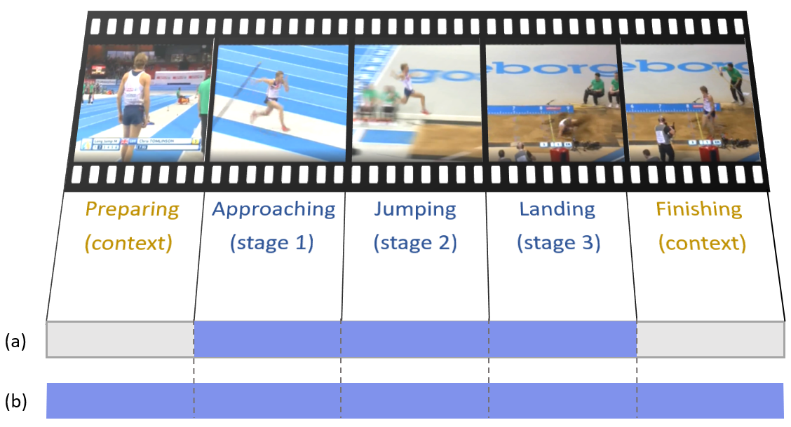
Both kinds of methods largely rely on the video-level classification model, which would lead to the intractable action-context confusion liu2019completeness issue in the absence of frame-wise labels. Take the long jump in Figure 1 as an example, the action has three stages, i.e., approaching, jumping, and landing. In addition, the frames before and after the action, i.e., preparing and finishing, contain the content that is closely related to long jump, but are not parts of the action. We refer to such frames as context, which is a special kind of background. In this example, the context parts include the track field and sandpit, which could in fact significantly encourage the recognition of the action. Without frame-wise annotations, the classifier is normally learned by aggregating the features of all related frames, where context and action are roughly mixed up. The context frames thus tend to be easily recognized as action frames themselves. The action-context confusion problem has not been fully studied though it is common in WSAL. One recent exploration liu2019completeness attempts to solve the problem by assuming a strong prior that context clips should be stationary, i.e., no motions in them. However, such assumption has massive limitations and ignores the inherent difference between context and action.
To separate context and action, the model should be able to capture the underlying discrepancy between them. Intuitively, context frame indeed exhibits obvious difference from action frame at the appearance or motion level. For example, among the five stages in Figure 1, the action stages (approaching, jumping, and landing) clearly demonstrate more intense body postures than the context stages (preparing and finishing). In other words, the extracted feature representations for context and action are also different. Such difference exists regardless of the action category.
Inspired by this observation, we propose a novel generative attention mechanism to model the frame representation conditioned on frame attention. In addition to the above intuition, we build a graphical model to theoretically demonstrate that the localization problem is associated with both the conventional classification and the proposed representation modeling. Our framework thus consists of two parts: the Discriminative and Generative Attention Modeling (DGAM). On one hand, the discriminative attention modeling trains a classification model on temporally pooled features weighted by the frame attention. On the other hand, a generative model, i.e., conditional Variational Auto-Encoder (VAE), is learned to model the class-agnostic frame-wise distribution of representation conditioned on attention values. By maximizing likelihood of the representation, the frame-wise attention is optimized accordingly, leading to well separation of action and context frames. Extensive experiments are conducted on THUMOS14 idrees2017thumos and ActivityNet1.2 caba2015activitynet to show that DGAM outperforms the state-of-the-arts by a significant margin. Comprehensive analysis further validates its effectiveness on separating action and context.
The main contribution of this work is the proposed DGAM framework for addressing the issue of action-context confusion in WSAL by modeling the frame representation conditioned on different attentions. The solution has led to elegant views of how localization is associated with the representation distribution and how to learn better attentions by modeling the representation, which have not been discussed in the literature.
2 Related Works
Video action recognition is a fundamental problem in video analytics. Most video-related tasks leverage the off-the-shelf action recognition models to extract features for further analysis. Early methods normally devise hand-crafted features laptev2005space; wang2013action; oneata2013action for recognition. Recently, thanks to the development of deep learning techniques, lots of approaches focus on automatic feature extraction with end-to-end learning, e.g., two-stream network simonyan2014two, temporal segment network (TSN) wang2016temporal, 3D ConvNet (C3D) tran2015learning, Pseudo 3D (P3D) qiu2017learning, Inflated 3D (I3D) carreira2017quo. In our experiments, I3D is utilized for feature extraction.
Fully-supervised action localization has been extensively studied recently. Many works follow the paradigms that are widely applied in object detection area girshick2014rich; girshick2015fast; ren2015faster; redmon2016you; liu2016ssd due to their commonalities in problem setting. To be more specific, there are mainly two directions, namely two-stage method and one-stage method. Two-stage methods zhao2017temporal; xu2017r; dai2017temporal; chao2018rethinking; shou2016temporal; shou2017cdc; gao2017cascaded; heilbron2017scc; lin2018bsn first generate action proposals and then classify them with further refinement on temporal boundaries. One-stage methods buch2017end; lin2017single; zhang2018s3d instead predict action category and location directly from raw data. In fully-supervised setting, the action-context confusion could be alleviated with frame-wise annotations.
Weakly-supervised action localization is drawing increasing attention due to the time-consuming manual labeling in fully-supervised setting. As introduced in Section 1, WSAL methods can be grouped into two categories, namely top-down and bottom-up methods. In top-down pipeline (e.g. UntrimmedNet wang2017untrimmednets), video-level classification model is learned first, and then frames with high classification activation are selected as action locations. W-TALC paul2018w and 3C-Net narayan20193c also force foreground features from the same class to be similar, otherwise dissimilar. Unlike top-down scheme, the bottom-up methods directly produce the attention for each frame from data, and train a classification model with the features weighted by attention. Based on this paradigm, STPN nguyen2018weakly further adds a regularization term to encourage the sparsity of action. AutoLoc shou2018autoloc proposes the Outer-Inner-Contrastive (OIC) loss by assuming that a complete action clip should look different from its neighbours. MAAN yuan2018marginalized proposes to suppress dominance of the most salient action frames and retrieve less salient ones. Nguyen et al. nguyen2019weakly propose to penalize the discriminative capacity of background, which is also utilized in our classification module. Besides, a video-level clustering loss is applied in nguyen2019weakly to separate foreground and background. Nevertheless, all of the aforementioned methods ignore the challenging action-context confusion issue caused by the absence of frame-wise label. Though Liu et al. liu2019completeness try to separate action and context using hard negative mining, their method is based on the strong assumption that context clips should be stationary, which has many limitations and may hence cause negative influence on the prediction.
Generative model has also experienced a fast development in recent years kingma2013auto; goodfellow2014generative; higgins2017beta. GAN goodfellow2014generative employs a generator to approximate real data distribution by the adversarial training between generator and discriminator. However, the learned approximating distribution is implicitly determined by generator and thus cannot be analytically expressed. VAE kingma2013auto approximates the real distribution by optimizing the variational lower bound on the marginal likelihood of data. Given a latent code, the conditional distribution is explicitly modeled as a Gaussian distribution, hence data distribution can be analytically expressed by sampling latent vectors and calculating the Gaussian. Flow-based model kingma2018glow uses invertible layers as the generative mapping, where data distribution can be calculated given the Jacobian of each layer. However, all layers must have the same dimensions, which is much less flexible. In our work, we exploit Conditional VAE (CVAE) sohn2015learning to model the frame feature distribution conditioned on attention value.
3 Method
Suppose we have a set of training videos and the corresponding video-level labels. For each video, we sample frames (snippets) to extract the RGB or optical flow features with a pre-trained model, where is the feature of frame , and is feature dimension. The video-level label is denoted as , where is the number of classes and corresponds to background. For brevity, we assume that each video only belongs to one class, though the following discussion can also apply to multi-label videos.
Our method follows the bottom-up pipeline for WSAL, which learns the attention directly from data, where is the attention of frame . Before discussing the details of our method, we examine the action localization problem from the beginning.
3.1 Attention-based Framework
In attention-based action localization problem, the target is to predict the frame attention , which is equivalent to solving the maximum a posteriori (MAP) problem:
| (1) |
where is the unknown probability distribution of given and . In the absence of frame-level labels (ground truth of ), it is difficult to approximate and optimize directly. Therefore, we transform the optimization target using Bayes' theorem,
| (2) |
where in the last step, we discard the constant term and assume a uniform prior of , i.e., . Our optimization problem thus becomes
| (3) |
This formulation indicates two different aspects for optimizing . The first term prefers with high discriminative capacity for action classification, which is the main optimization target in previous works. In contrast, the second term forces the representation of frames to be accurately predicted from the attention . Given the feature difference between foreground and background, this objective encourages the model to impose different attentions on different features. In specific, we exploit a generative model to approximate , and force the feature to be accurately reconstructed by the model.
Figure 2 shows the graphical model of the above problem. The model parameters () and the latent variables in generative model () will be discussed later. Based on (3), the framework of our method consists of two components, i.e., the discriminative attention modeling and the generative attention modeling, as illustrated in Figure 3.
3.2 Discriminative Attention Modeling
The discriminative attention module learns the frame attention by optimizing the video-level recognition task. In specific, we utilize attention as weight to perform temporal average pooling over all frames in the video and produce a video-level foreground feature given by
| (4) |
Similarly, we can also utilize as the weight to calculate a background feature :
| (5) |
To optimize , we encourage high discriminative capability of the foreground feature and simultaneously punish any discriminative capability of the background feature nguyen2019weakly. This is equivalent to minimizing the following discriminative loss (i.e. softmax loss):
| (6) |
where is a hyper-parameter, and is our classification module modeled by a fully-connected layer with weight for each class and a following softmax layer. During training, attention module and classification module are jointly optimized. The graphical model of this part is illustrated in Figure 2 with dash-dot lines.
3.3 Generative Attention Modeling
The discriminative attention optimization generally has difficulty in separating context and foreground when frame-wise annotations are unavailable. Based on the observation that context differs from foreground in terms of feature representation, we utilize a Conditional Variational Auto-Encoder (CVAE) to model the representation distribution of different frames. Before explaining the details, we briefly review the Variational Auto-Encoder (VAE).
Given the observed variable , VAE kingma2013auto introduces a latent variable , and aims to generate from , i.e.,
| (7) |
where denotes the parameters of generative model, is the prior (e.g. a standard Gaussian), and is the conditional distribution indicating the generation procedure, which is typically estimated with a neural network that is referred to as decoder. The key idea behind is to sample values of that are likely to produce , which means that we need an approximation to the intractable posterior . denotes the parameters of approximation model, and is also estimated via a neural network , which is referred to as encoder. VAE incorporates encoder and decoder , and learns parameters by maximizing the variational lower bound:
| (8) |
where is the KL divergence of from .
In our DGAM model, we expect to generate the observation based on the attention , i.e., , which can be written as by assuming independence between frames in a video. Similarly, we introduce a latent variable , and attempt to generate each from and , which forms a Conditional VAE problem:
| (9) |
Note that the desired distribution of is modeled as a Gaussian, i.e., , where is the decoder, is a hyper-parameter, and is the unit matrix. Ideally, is sampled from the prior . In DGAM, we set the prior as a Gaussian, i.e., , where is all-ones vector and is a hyper-parameter indicating the discrepancy between priors of different attention value . When , prior is independent of .
During training of CVAE, we also approximate the intractable posterior by a Gaussian , where and are the outputs of the encoder . We then minimize the variational loss :
| (10) |
where is -th sample from . Note that the Monte Carlo estimation of the expectation is employed with samples. is a hyper-parameter for trade-off between reconstruction quality and sampling accuracy.
For the generative attention modeling of , we fix CVAE and minimize the reconstruction loss given by
| (11) |
where is sampled from the prior . In our experiments, is set to , and (11) can be written as
| (12) |
The graphical model of generative attention modeling is illustrated in Figure 2 with solid and dashed lines.
In our framework, the CVAE cannot be directly and solely optimized due to the unavailability of ground truth . Therefore, we propose to train attention module and CVAE in an alternating way, i.e., we first update CVAE with “pseudo label” of given by the attention module, and then train attention module with fixed CVAE. The two stages are repeated for several iterations. Since there exist other loss terms for attention modeling (e.g. ), the pseudo label can be high-quality and hence a good convergence can be reached. Experimental results empirically validate it.
3.4 Optimization
In addition to the above objectives, we exploit a self-guided regularization nguyen2019weakly to further refine the attention. The temporal class activation maps (TCAM) nguyen2018weakly; zhou2016learning are utilized to produce the top-down, class-aware attention maps. In specific, given a video with label , the TCAM are computed by
| (13) | ||||
| (14) |
where indicates the parameters of the classification module for class . and are foreground and background TCAM, respectively. is a Gaussian smooth filter with standard deviation , and represents convolution. The generated and are expected to be consistent with the bottom-up, class-agnostic attention , hence the loss can be formulated as
| (15) |
To sum up, we optimize the whole framework by alternately executing the following two steps:
- 1.
Update attention and classification modules with loss
(16) where denote the hyper-parameters.
- 2.
Update CVAE with loss .
The whole architecture is illustrated in Figure 3.
3.5 Action Prediction
To generate action proposals for a video during inference, we feed the video to DGAM and obtain the attention . By filtering out frames with attention lower than a threshold , we extract consecutive segments with high attention values as the predicted locations. For each segment , we temporally pool the features with attention, and get the classification score for class , which is the output of classification module before softmax. We further follow shou2018autoloc; liu2019completeness to refine by subtracting the score of its surroundings. The final score is calculated by
| (17) |
where is the subtraction parameter.
4 Experiments
4.1 Datasets and Evaluation Metrics
For evaluation, we conduct experiments on two benchmarks, THUMOS14 idrees2017thumos and ActivityNet1.2 caba2015activitynet. During training, only video-level category labels are available.
THUMOS14 contains videos from 20 classes for action localization task. We follow the convention to train on validation set with 200 videos and evaluate on test set with 212 videos. Note that we exclude the wrongly annotated video#270 from test set, following nguyen2019weakly; zhao2017temporal. This dataset is challenging for its finely annotated action instances. Each video contains 15.5 action clips on average. Length of action instance varies widely, from a few seconds to minutes. Video length also ranges from a few seconds to 26 minutes, with an average of around 3 minutes. Compared to other large-scale datasets, e.g., ActivityNet1.2, THUMOS14 has less training data which indicates higher requirement of model’s generalization ability and robustness.
ActivtyNet1.2 contains 100 classes of videos with both video-level labels and temporal annotations. Each video contains 1.5 action instances on average. Following wang2017untrimmednets; shou2018autoloc, we train our model on training set with 4819 videos and evaluate on validation set with 2383 videos.
Evaluation Metrics. We follow the standard evaluation protocol and report mean Average Precision (mAP) at different intersection over union (IoU) thresholds. The results are calculated using the benchmark code provided by ActivityNet official codebase22 2 https://github.com/activitynet/ActivityNet/tree/master/Evaluation. For fair comparison, all results on THUMOS14 are averaged over five runs.
| Att | Cls | mAP@IoU | ||||
|---|---|---|---|---|---|---|
| 0.3 | 0.4 | 0.5 | 0.6 | 0.7 | ||
| O | O | 43.8 | 35.8 | 26.7 | 18.2 | 9.7 |
| O | N | 44.2 | 36.1 | 27.0 | 18.7 | 9.8 |
| N | O | 46.1 | 38.2 | 28.8 | 19.4 | 11.2 |
| N | N | 46.8 | 38.2 | 28.8 | 19.8 | 11.4 |
4.2 Implementation Details
We utilize I3D carreira2017quo network pre-trained on Kinetics kay2017kinetics as the feature extractor33 3 https://github.com/deepmind/kinetics-i3d. In specific, we first extract optical flow from RGB data using TV-L1 algorithm perez2013tv. Then we divide both streams into non-overlapping 16-frame snippets and send them into the pre-trained I3D network to obtain two 1024-dimension feature frames for each snippet. We train separate DGAMs for RGB and flow streams. The proposals from them are combined with Non-Maximum Suppression (NMS) during inference. Following nguyen2018weakly; nguyen2019weakly, we set to 400 for all videos during training. During evaluation, we feed all frames of each video to our network if the frame number is less than , otherwise we sample frames uniformly. is 400 for THUMOS14, and 200 for ActivityNet1.2.
We set in Eq. (6) and in Eq. (10). In Eq. (16), we set to for RGB stream, and for flow stream. is set as . The whole architecture is implemented with PyTorch paszke2017automatic and trained on single NVIDIA Tesla M40 GPU using Adam optimizer kingma2014adam with learning rate of . To stabilize the training of DGAM, we leverage a warm-up strategy in the first 300 epochs when updating and .
| Metric | w/o | w/ | |
|---|---|---|---|
| 0.777 | 0.698 | ||
| 0.858 | 0.707 | ||
| 1.522 | 1.543 | ||
| 0.001 | 0.001 |
| Method | Supervision | Feature | mAP@IoU | ||||||||
|---|---|---|---|---|---|---|---|---|---|---|---|
| 0.1 | 0.2 | 0.3 | 0.4 | 0.5 | 0.6 | 0.7 | 0.8 | 0.9 | |||
| S-CNN shou2016temporal | Full | - | 47.7 | 43.5 | 36.3 | 28.7 | 19.0 | 10.3 | 5.3 | - | - |
| R-C3D xu2017r | Full | - | 54.5 | 51.5 | 44.8 | 35.6 | 28.9 | - | - | - | - |
| SSN zhao2017temporal | Full | - | 66.0 | 59.4 | 51.9 | 41.0 | 29.8 | - | - | - | - |
| Chao et al. chao2018rethinking | Full | - | 59.8 | 57.1 | 53.2 | 48.5 | 42.8 | 33.8 | 20.8 | - | - |
| BSN lin2018bsn | Full | - | - | - | 53.5 | 45.0 | 36.9 | 28.4 | 20.0 | - | - |
| P-GCN zeng2019graph | Full | - | 69.5 | 67.8 | 63.6 | 57.8 | 49.1 | - | - | - | - |
| Hide-and-Seek singh2017hide | Weak | - | 36.4 | 27.8 | 19.5 | 12.7 | 6.8 | - | - | - | - |
| UntrimmedNet wang2017untrimmednets | Weak | - | 44.4 | 37.7 | 28.2 | 21.1 | 13.7 | - | - | - | - |
| Zhong et al. zhong2018step | Weak | - | 45.8 | 39.0 | 31.1 | 22.5 | 15.9 | - | - | - | - |
| AutoLoc shou2018autoloc | Weak | UNT | - | - | 35.8 | 29.0 | 21.2 | 13.4 | 5.8 | - | - |
| CleanNet liuweakly | Weak | UNT | - | - | 37.0 | 30.9 | 23.9 | 13.9 | 7.1 | - | - |
| STPN nguyen2018weakly | Weak | I3D | 52.0 | 44.7 | 35.5 | 25.8 | 16.9 | 9.9 | 4.3 | 1.2 | 0.1 |
| MAAN yuan2018marginalized | Weak | I3D | 59.8 | 50.8 | 41.1 | 30.6 | 20.3 | 12.0 | 6.9 | 2.6 | 0.2 |
| W-TALC paul2018w | Weak | I3D | 55.2 | 49.6 | 40.1 | 31.1 | 22.8 | - | 7.6 | - | - |
| Liu et al. liu2019completeness | Weak | I3D | 57.4 | 50.8 | 41.2 | 32.1 | 23.1 | 15.0 | 7.0 | - | - |
| TSM yutemporal | Weak | I3D | - | - | 39.5 | - | 24.5 | - | 7.1 | - | - |
| 3C-Net narayan20193c | Weak | I3D | 56.8 | 49.8 | 40.9 | 32.3 | 24.6 | - | 7.7 | - | - |
| Nguyen et al. nguyen2019weakly | Weak | I3D | 60.4 | 56.0 | 46.6 | 37.5 | 26.8 | 17.6 | 9.0 | 3.3 | 0.4 |
| DGAM | Weak | I3D | 60.0 | 54.2 | 46.8 | 38.2 | 28.8 | 19.8 | 11.4 | 3.6 | 0.4 |
4.3 Statistical Evaluation on Attention
We first evaluate the learned attention of DGAM and its effectiveness on handling action-context confusion. For comparison, an “old” model is trained by removing the generative attention modeling (GAM) from DGAM, and our DGAM is denoted as the “new” model. Note that only Attention and Classification modules are involved during inference. When evaluating, we assemble specific models by alternately choosing the two modules from “old” or “new” models. Table 1 details the mAP results on THUMOS14. It can be found that the new attention module largely improves the performance, while there is little or no improvement with the new classification module. This observation indicates that DGAM indeed learns better attention values. Even with “old” classifier, the “new” attention can boost the localization significantly.
We further collect several statistics to show the improvement intuitively in Table 2. Experiments are conducted on both “old” (w/o GAM) and “new” (w/ GAM) models. In particular, att (cls) indicates the set of frames with attention values (classification scores) larger than a threshold , and gt is the set of ground truth frames. represents size of a set. ‘’, ‘’ and ‘’ indicate set exclusion, intersection and complement, separately. Though such simple thresholding is not exactly the predicted locations, it somewhat reflects the quality of localization.
In Table 2, or indicates the percentage of frames falsely captured or omitted by attention. It shows that both false activation and omission can be reduced with GAM. Moreover, an improvement in demonstrates that GAM can better filter out the false positives (e.g. context frames) made by classifier. measures how attention can capture the false negatives, i.e., action frames neglected by classifier. Since GAM is devised for excluding the false positives produced by classifier, it is not surprising that GAM contributes little to it.
| mAP@0.5 | ||||
|---|---|---|---|---|
| ✓ | - | - | - | 21.5 |
| ✓ | ✓ | - | - | 24.8 |
| ✓ | ✓ | ✓ | - | 26.7 |
| ✓ | ✓ | ✓ | ✓ | 28.8 |
4.4 Ablation Studies
Next we study how each component in DGAM influences the overall performance. We start with the basic model that directly optimizes the attention based foreground classification loss . The background classification loss , the self-guided regularization loss , and the feature reconstruction loss are further included step by step. Note that adding indicates involving the generative attention modeling, where is also optimized.
Table 4 summarizes the performance by considering one more factor at each stage on THUMOS14. Background classification is a general approach for both video recognition and localization. In our case, it is part of our discriminative attention modeling, which brings a performance gain of 3.3%. Self-guided regularization is the additional optimization of our system, which leads to 1.9% mAP improvement. Our generative attention modeling further contributes a significant increase of 2.1% and the performance of DGAM finally reaches 28.8%.
| Method | Supervision | mAP@IoU | ||||||||||
|---|---|---|---|---|---|---|---|---|---|---|---|---|
| 0.5 | 0.55 | 0.6 | 0.65 | 0.7 | 0.75 | 0.8 | 0.85 | 0.9 | 0.95 | AVG | ||
| SSN zhao2017temporal | Full | 41.3 | 38.8 | 35.9 | 32.9 | 30.4 | 27.0 | 22.2 | 18.2 | 13.2 | 6.1 | 26.6 |
| UntrimmedNet∗ wang2017untrimmednets | Weak | 7.4 | 6.1 | 5.2 | 4.5 | 3.9 | 3.2 | 2.5 | 1.8 | 1.2 | 0.7 | 3.6 |
| AutoLoc∗ shou2018autoloc | Weak | 27.3 | 24.9 | 22.5 | 19.9 | 17.5 | 15.1 | 13.0 | 10.0 | 6.8 | 3.3 | 16.0 |
| W-TALC paul2018w | Weak | 37.0 | 33.5 | 30.4 | 25.7 | 14.6 | 12.7 | 10.0 | 7.0 | 4.2 | 1.5 | 18.0 |
| TSM yutemporal | Weak | 28.3 | 26.0 | 23.6 | 21.2 | 18.9 | 17.0 | 14.0 | 11.1 | 7.5 | 3.5 | 17.1 |
| 3C-Net narayan20193c | Weak | 35.4 | - | - | - | 22.9 | - | - | - | 8.5 | - | 21.1 |
| CleanNet liuweakly | Weak | 37.1 | 33.4 | 29.9 | 26.7 | 23.4 | 20.3 | 17.2 | 13.9 | 9.2 | 5.0 | 21.6 |
| Liu et al. liu2019completeness | Weak | 36.8 | - | - | - | - | 22.0 | - | - | - | 5.6 | 22.4 |
| DGAM | Weak | 41.0 | 37.5 | 33.5 | 30.1 | 26.9 | 23.5 | 19.8 | 15.5 | 10.8 | 5.3 | 24.4 |
| (dim) | 4 | 5 | 6 | 7 | 8 | 9 |
|---|---|---|---|---|---|---|
| mAP@0.5 | 26.5 | 27.5 | 28.0 | 28.8 | 28.3 | 27.7 |
| 0.01 | 0.03 | 0.07 | 0.1 | 0.3 | 0.7 | |
|---|---|---|---|---|---|---|
| mAP@0.5 | 28.2 | 28.1 | 28.4 | 28.8 | 28.0 | 28.4 |
4.5 Evaluation on Parameters
To further understand the proposed model, we conduct evaluations to analyze the impact of different parameter settings in DGAM. mAP@ on THUMOS14 is reported.
Discrepancy between latent prior of different . In generative attention modeling, different attentions correspond to different feature distributions . The discrepancy between these distributions can be implicitly modeled by the discrepancy between latent codes sampled from different priors, which are modeled as different Gaussian distributions . Here controls the discrepancy. We evaluate every 0.25 from 0 to 1.5, and the results are shown in Figure 4. In general, the performance is relatively stable with small fluctuation, demonstrating the robustness of DGAM.
Dimension of latent space. The dimension of latent space in CVAE is crucial for quality of reconstruction and complexity of modeled distribution. High dimension can facilitate the approximation of feature distribution, hence leading to more accurate attention learning. However, more training data is also required. We evaluate different dimensions of , . As shown in Table 6, mAP improves rapidly with increasing dimension, which indicates better generative attention modeling. The result reaches the peak at dimension . After that, the performance starts dropping, partially because of the sparsity of limited data in high-dimensional latent space.
Reconstruction-sampling trade-off in CVAE. The hyper-parameter in Eq. (10) balances reconstruction quality (the first term) and sampling accuracy (the second term). With larger , we expect the approximated posterior to be closer to the prior, which improves the precision when sampling latent vectors from prior, while the reconstruction quality (i.e. the quality of learned distribution) will decrease. We test different from 0 to 1. As shown in Table 7, the performance fluctuates in a small range from 28% to 28.8%, indicating that our method is insensitive to .
4.6 Comparisons with State-of-the-Art
Table 3 compares our DGAM with existing approaches in both weakly-supervised and fully-supervised action localization on THUMOS14. Our method outperforms other weakly-supervised methods, especially at high IoU threshold, which means DGAM could produce finer and more precise predictions. Compared with state of the art, DGAM improves mAP at IoU=0.5 by 2%. Note that Nguyen et al. nguyen2019weakly achieves better performance at IoU=0.1 and 0.2 than our model, partially because our generative attention modeling may discard out-of-distribution hard candidates (outliers), which become common when IoU is low. Furthermore, our results are comparable with several fully-supervised methods, indicating the effectiveness of the proposed DGAM.
On ActivityNet1.2, we summarize the performance comparisons in Table 5. Our method significantly outperforms the state-of-the-arts. Particularly, DGAM surpasses the best competitor by 2% on mAP@AVG. Our method also demonstrates comparable results to fully-supervised methods.
5 Conclusion
We have presented a novel Discriminative and Generative Attention Modeling (DGAM) method to solve the action-context confusion issue in weakly-supervised action localization. Particularly, we study the problem of modeling frame-wise attention based on the distribution of frame features. With the observation that context feature obviously differs from action feature, we devise a conditional variation auto-encoder (CVAE) to construct different feature distributions conditioned on different attentions. The learned CVAE in turn refines the desired frame-wise attention according to their features. Experiments conducted on two benchmarks, i.e., THUMOS14 and ActivityNet1.2, validate our method and analysis. More remarkably, we achieve the new state-of-the-art results on both datasets.
Acknowledgements This work is supported by Beijing Municipal Commission of Science and Technology under Grant Z181100008918005, National Natural Science Foundation of China (NSFC) under Grant 61772037. Baifeng Shi thanks Prof. Tingting Jiang and Daochang Liu for enlightening discussions.
References
- (1) Humam Alwassel, Fabian Caba Heilbron, and Bernard Ghanem. Action search: Spotting actions in videos and its application to temporal action localization. In Proceedings of the European Conference on Computer Vision (ECCV), pages 251–266, 2018.
- (2) Shyamal Buch, Victor Escorcia, Bernard Ghanem, Li Fei-Fei, and Juan Carlos Niebles. End-to-end, single-stream temporal action detection in untrimmed videos. In British Machine Vision Conference (BMVC), volume 2, page 7, 2017.
- (3) Fabian Caba Heilbron, Victor Escorcia, Bernard Ghanem, and Juan Carlos Niebles. Activitynet: A large-scale video benchmark for human activity understanding. In Proceedings of the IEEE Conference on Computer Vision and Pattern Recognition (CVPR), pages 961–970, 2015.
- (4) Joao Carreira and Andrew Zisserman. Quo vadis, action recognition? a new model and the kinetics dataset. In Proceedings of the IEEE Conference on Computer Vision and Pattern Recognition (CVPR), pages 6299–6308, 2017.
- (5) Yu-Wei Chao, Sudheendra Vijayanarasimhan, Bryan Seybold, David A Ross, Jia Deng, and Rahul Sukthankar. Rethinking the faster r-cnn architecture for temporal action localization. In Proceedings of the IEEE Conference on Computer Vision and Pattern Recognition (CVPR), pages 1130–1139, 2018.
- (6) Xiyang Dai, Bharat Singh, Guyue Zhang, Larry S Davis, and Yan Qiu Chen. Temporal context network for activity localization in videos. In Proceedings of the IEEE International Conference on Computer Vision (ICCV), pages 5793–5802, 2017.
- (7) Jiyang Gao, Zhenheng Yang, and Ram Nevatia. Cascaded boundary regression for temporal action detection. In British Machine Vision Conference (BMVC), 2017.
- (8) Ross Girshick. Fast r-cnn. In Proceedings of the IEEE International Conference on Computer Vision (ICCV), pages 1440–1448, 2015.
- (9) Ross Girshick, Jeff Donahue, Trevor Darrell, and Jitendra Malik. Rich feature hierarchies for accurate object detection and semantic segmentation. In Proceedings of the IEEE Conference on Computer Vision and Pattern Recognition (CVPR), pages 580–587, 2014.
- (10) Ian Goodfellow, Jean Pouget-Abadie, Mehdi Mirza, Bing Xu, David Warde-Farley, Sherjil Ozair, Aaron Courville, and Yoshua Bengio. Generative adversarial nets. In Advances in neural information processing systems (NeurIPS), pages 2672–2680, 2014.
- (11) Fabian Caba Heilbron, Wayner Barrios, Victor Escorcia, and Bernard Ghanem. Scc: Semantic context cascade for efficient action detection. In 2017 IEEE Conference on Computer Vision and Pattern Recognition (CVPR), pages 3175–3184. IEEE, 2017.
- (12) Irina Higgins, Loic Matthey, Arka Pal, Christopher Burgess, Xavier Glorot, Matthew Botvinick, Shakir Mohamed, and Alexander Lerchner. beta-vae: Learning basic visual concepts with a constrained variational framework. In Proceedings of the International Conference on Learning Representations (ICLR), 2017.
- (13) Haroon Idrees, Amir R Zamir, Yu-Gang Jiang, Alex Gorban, Ivan Laptev, Rahul Sukthankar, and Mubarak Shah. The thumos challenge on action recognition for videos “in the wild”. Computer Vision and Image Understanding (CVIU), 155:1–23, 2017.
- (14) Will Kay, Joao Carreira, Karen Simonyan, Brian Zhang, Chloe Hillier, Sudheendra Vijayanarasimhan, Fabio Viola, Tim Green, Trevor Back, Paul Natsev, et al. The kinetics human action video dataset. arXiv preprint arXiv:1705.06950, 2017.
- (15) Diederik P Kingma and Jimmy Ba. Adam: A method for stochastic optimization. In Proceedings of the International Conference on Learning Representations (ICLR), 2014.
- (16) Diederik P Kingma and Prafulla Dhariwal. Glow: Generative flow with invertible 1x1 convolutions. In Advances in Neural Information Processing Systems (NeurIPS), pages 10215–10224, 2018.
- (17) Diederik P Kingma and Max Welling. Auto-encoding variational bayes. In Proceedings of the International Conference on Learning Representations (ICLR), 2013.
- (18) Alex Krizhevsky, Ilya Sutskever, and Geoffrey E Hinton. Imagenet classification with deep convolutional neural networks. In Advances in neural information processing systems (NeurIPS), pages 1097–1105, 2012.
- (19) Ivan Laptev. On space-time interest points. International Journal of Computer Vision (IJCV), 64(2-3):107–123, 2005.
- (20) Dong Li, Zhaofan Qiu, Qi Dai, Ting Yao, and Tao Mei. Recurrent tubelet proposal and recognition networks for action detection. In Proceedings of the European conference on computer vision (ECCV), pages 303–318, 2018.
- (21) Dong Li, Ting Yao, Zhaofan Qiu, Houqiang Li, and Tao Mei. Long short-term relation networks for video action detection. In Proceedings of the ACM International Conference on Multimedia (MM), pages 629–637, 2019.
- (22) Tianwei Lin, Xu Zhao, and Zheng Shou. Single shot temporal action detection. In Proceedings of the ACM international conference on Multimedia (MM), pages 988–996. ACM, 2017.
- (23) Tianwei Lin, Xu Zhao, Haisheng Su, Chongjing Wang, and Ming Yang. Bsn: Boundary sensitive network for temporal action proposal generation. In Proceedings of the European Conference on Computer Vision (ECCV), pages 3–19, 2018.
- (24) Daochang Liu, Tingting Jiang, and Yizhou Wang. Completeness modeling and context separation for weakly supervised temporal action localization. In Proceedings of the IEEE Conference on Computer Vision and Pattern Recognition (CVPR), pages 1298–1307, 2019.
- (25) Wei Liu, Dragomir Anguelov, Dumitru Erhan, Christian Szegedy, Scott Reed, Cheng-Yang Fu, and Alexander C Berg. Ssd: Single shot multibox detector. In European Conference on Computer Vision (ECCV), pages 21–37. Springer, 2016.
- (26) Ziyi Liu, Le Wang, Qilin Zhang, Zhanning Gao, Zhenxing Niu, Nanning Zheng, and Gang Hua. Weakly supervised temporal action localization through contrast based evaluation networks. In Proceedings of the IEEE International Conference on Computer Vision (ICCV), pages 3899–3908, 2019.
- (27) Fuchen Long, Ting Yao, Zhaofan Qiu, Xinmei Tian, Jiebo Luo, and Tao Mei. Gaussian temporal awareness networks for action localization. In Proceedings of the IEEE Conference on Computer Vision and Pattern Recognition (CVPR), pages 344–353, 2019.
- (28) Yu-Fei Ma, Xian-Sheng Hua, Lie Lu, and Hong-Jiang Zhang. A generic framework of user attention model and its application in video summarization. IEEE Transaction on multimedia (TMM), 7(5):907–919, 2005.
- (29) Sanath Narayan, Hisham Cholakkal, Fahad Shahbaz Khan, and Ling Shao. 3c-net: Category count and center loss for weakly-supervised action localization. In Proceedings of the IEEE International Conference on Computer Vision (ICCV), pages 8679–8687, 2019.
- (30) Phuc Nguyen, Ting Liu, Gautam Prasad, and Bohyung Han. Weakly supervised action localization by sparse temporal pooling network. In Proceedings of the IEEE Conference on Computer Vision and Pattern Recognition (CVPR), pages 6752–6761, 2018.
- (31) Phuc Xuan Nguyen, Deva Ramanan, and Charless C Fowlkes. Weakly-supervised action localization with background modeling. In Proceedings of the IEEE International Conference on Computer Vision (ICCV), pages 5502–5511, 2019.
- (32) Dan Oneata, Jakob Verbeek, and Cordelia Schmid. Action and event recognition with fisher vectors on a compact feature set. In Proceedings of the IEEE International Conference on Computer Vision (ICCV), pages 1817–1824, 2013.
- (33) Adam Paszke, Sam Gross, Soumith Chintala, Gregory Chanan, Edward Yang, Zachary DeVito, Zeming Lin, Alban Desmaison, Luca Antiga, and Adam Lerer. Automatic differentiation in PyTorch. In NeurIPS Autodiff Workshop, 2017.
- (34) Sujoy Paul, Sourya Roy, and Amit K Roy-Chowdhury. W-talc: Weakly-supervised temporal activity localization and classification. In Proceedings of the European Conference on Computer Vision (ECCV), pages 563–579, 2018.
- (35) Javier Sánchez Pérez, Enric Meinhardt-Llopis, and Gabriele Facciolo. Tv-l1 optical flow estimation. Image Processing On Line (IPOL), 2013:137–150, 2013.
- (36) Zhaofan Qiu, Ting Yao, and Tao Mei. Learning spatio-temporal representation with pseudo-3d residual networks. In Proceedings of the IEEE International Conference on Computer Vision (ICCV), pages 5533–5541, 2017.
- (37) Zhaofan Qiu, Ting Yao, Chong-Wah Ngo, Xinmei Tian, and Tao Mei. Learning spatio-temporal representation with local and global diffusion. In Proceedings of the IEEE Conference on Computer Vision and Pattern Recognition (CVPR), pages 12056–12065, 2019.
- (38) Joseph Redmon, Santosh Divvala, Ross Girshick, and Ali Farhadi. You only look once: Unified, real-time object detection. In Proceedings of the IEEE Conference on Computer Vision and Pattern Recognition (CVPR), pages 779–788, 2016.
- (39) Shaoqing Ren, Kaiming He, Ross Girshick, and Jian Sun. Faster r-cnn: Towards real-time object detection with region proposal networks. In Advances in neural information processing systems (NeurIPS), pages 91–99, 2015.
- (40) Zheng Shou, Jonathan Chan, Alireza Zareian, Kazuyuki Miyazawa, and Shih-Fu Chang. Cdc: Convolutional-de-convolutional networks for precise temporal action localization in untrimmed videos. In Proceedings of the IEEE Conference on Computer Vision and Pattern Recognition (CVPR), pages 5734–5743, 2017.
- (41) Zheng Shou, Hang Gao, Lei Zhang, Kazuyuki Miyazawa, and Shih-Fu Chang. Autoloc: Weakly-supervised temporal action localization in untrimmed videos. In Proceedings of the European Conference on Computer Vision (ECCV), pages 154–171, 2018.
- (42) Zheng Shou, Dongang Wang, and Shih-Fu Chang. Temporal action localization in untrimmed videos via multi-stage cnns. In Proceedings of the IEEE Conference on Computer Vision and Pattern Recognition (CVPR), pages 1049–1058, 2016.
- (43) Karen Simonyan and Andrew Zisserman. Two-stream convolutional networks for action recognition in videos. In Advances in neural information processing systems (NeurIPS), pages 568–576, 2014.
- (44) Krishna Kumar Singh and Yong Jae Lee. Hide-and-seek: Forcing a network to be meticulous for weakly-supervised object and action localization. In 2017 IEEE International Conference on Computer Vision (ICCV), pages 3544–3553. IEEE, 2017.
- (45) Kihyuk Sohn, Honglak Lee, and Xinchen Yan. Learning structured output representation using deep conditional generative models. In Advances in neural information processing systems (NeurIPS), pages 3483–3491, 2015.
- (46) Du Tran, Lubomir Bourdev, Rob Fergus, Lorenzo Torresani, and Manohar Paluri. Learning spatiotemporal features with 3d convolutional networks. In Proceedings of the IEEE International Conference on Computer Vision (ICCV), pages 4489–4497, 2015.
- (47) Sarvesh Vishwakarma and Anupam Agrawal. A survey on activity recognition and behavior understanding in video surveillance. The Visual Computer (Vis Comput), 29(10):983–1009, 2013.
- (48) Heng Wang and Cordelia Schmid. Action recognition with improved trajectories. In Proceedings of the IEEE International Conference on Computer Vision (ICCV), pages 3551–3558, 2013.
- (49) Limin Wang, Yuanjun Xiong, Dahua Lin, and Luc Van Gool. Untrimmednets for weakly supervised action recognition and detection. In Proceedings of the IEEE conference on Computer Vision and Pattern Recognition (CVPR), pages 4325–4334, 2017.
- (50) Limin Wang, Yuanjun Xiong, Zhe Wang, Yu Qiao, Dahua Lin, Xiaoou Tang, and Luc Van Gool. Temporal segment networks: Towards good practices for deep action recognition. In European Conference on Computer Vision (ECCV), pages 20–36. Springer, 2016.
- (51) Bo Xiong, Yannis Kalantidis, Deepti Ghadiyaram, and Kristen Grauman. Less is more: Learning highlight detection from video duration. In Proceedings of the IEEE Conference on Computer Vision and Pattern Recognition (CVPR), pages 1258–1267, 2019.
- (52) Huijuan Xu, Abir Das, and Kate Saenko. R-c3d: Region convolutional 3d network for temporal activity detection. In Proceedings of the IEEE International Conference on Computer Vision (ICCV), pages 5783–5792, 2017.
- (53) Serena Yeung, Olga Russakovsky, Greg Mori, and Li Fei-Fei. End-to-end learning of action detection from frame glimpses in videos. In Proceedings of the IEEE Conference on Computer Vision and Pattern Recognition (CVPR), pages 2678–2687, 2016.
- (54) Tan Yu, Zhou Ren, Yuncheng Li, Enxu Yan, Ning Xu, and Junsong Yuan. Temporal structure mining for weakly supervised action detection. In Proceedings of the IEEE International Conference on Computer Vision (ICCV), pages 5522–5531, 2019.
- (55) Yuan Yuan, Yueming Lyu, Xi Shen, Ivor W. Tsang, and Dit-Yan Yeung. Marginalized average attentional network for weakly-supervised learning. In International Conference on Learning Representations (ICLR), 2019.
- (56) Runhao Zeng, Wenbing Huang, Mingkui Tan, Yu Rong, Peilin Zhao, Junzhou Huang, and Chuang Gan. Graph convolutional networks for temporal action localization. In Proceedings of the IEEE International Conference on Computer Vision (ICCV), pages 7094–7103, 2019.
- (57) Da Zhang, Xiyang Dai, Xin Wang, and Yuan-Fang Wang. S3d: Single shot multi-span detector via fully 3d convolutional network. In Proceedings of the British Machine Vision Conference (BMVC), 2018.
- (58) Yue Zhao, Yuanjun Xiong, Limin Wang, Zhirong Wu, Xiaoou Tang, and Dahua Lin. Temporal action detection with structured segment networks. In Proceedings of the IEEE International Conference on Computer Vision (ICCV), pages 2914–2923, 2017.
- (59) Jia-Xing Zhong, Nannan Li, Weijie Kong, Tao Zhang, Thomas H Li, and Ge Li. Step-by-step erasion, one-by-one collection: A weakly supervised temporal action detector. In Proceedings of the ACM international conference on Multimedia (MM), pages 35–44. ACM, 2018.
- (60) Bolei Zhou, Aditya Khosla, Agata Lapedriza, Aude Oliva, and Antonio Torralba. Learning deep features for discriminative localization. In Proceedings of the IEEE conference on Computer Vision and Pattern Recognition (CVPR), pages 2921–2929, 2016.