跳到论文正文
W Papers独立论文阅读器 arXiv:2003.12369 论文正文 计算阅读时间 · 0%
引用这篇论文根据当前论文元数据生成,正式投稿前建议核对。


License: arXiv.org perpetual non-exclusive license
arXiv:2003.12369v1 [math.NA] 27 Mar 2020

Solving quasistatic contact problems
using nonsmooth optimization approach

Michal Jureczka11 1 Jagiellonian University in Krakow, Faculty of Mathematics and Computer Science, Lojasiewicza 6, 30-348 Krakow, Poland. Email: michal.jureczka@uj.edu.pl,   Anna Ochal22 2 Jagiellonian University in Krakow, Faculty of Mathematics and Computer Science, Lojasiewicza 6, 30-348 Krakow, Poland. Email: ochal@ii.uj.edu.pl   and    Weimin Han33 3 Program in Applied Mathematical and Computational Sciences (AMCS) & Department of Mathematics, University of Iowa, Iowa City, IA 52242, USA. Email: weimin-han@uiowa.edu

Abstract. This paper is devoted to a study of time-dependent hemivariational inequality. We prove existence and uniqueness of its solution, provide fully discrete scheme and reformulate this scheme as a series of nonsmooth optimization problems. This theory is later applied to a sample quasistatic contact problem describing a viscoelastic body in frictional contact with a foundation. This contact is governed by a nonmonotone friction law with dependence on normal component of displacement and tangential component of velocity. Finally, computational simulations are performed to illustrate obtained results.

Keywords. Nonmonotone friction, optimization problem, error estimate, finite element method, numerical simulations.

AMS Classification. 35Q74, 49J40, 65K10, 65M60, 74S05, 74M15, 74M10, 74G15

1 Introduction

Currently various engineering applications require scientific analysis of contact phenomena. In order to study such problems a framework in the form of variational and hemivariational inequalities complemented by theory of Finite Element Method emerged. Literature in the field of Contact Mechanics grows rapidly. Main ideas and mathematical tools were introduced in monographs [6, 14, 17, 18, 20]. Other comprehensive studies include [10, 19, 21, 22]. Theory of nonsmooth optimization used in our approach was presented in [1] and applied to a sample static contact problem in [2]. Numerical analysis of contact problems can be found for instance in papers [3, 8, 9, 12, 13, 16] and for a recent study [11].

This paper is a continuation of our previous work [15], where we reformulated time-independent hemivariational inequality as optimization problem and used it to solve a static mechanical contact problem. Here, we consider time-dependent hemivariational inequality, and use similar idea to solve it numerically. In this case we prove existence and uniqueness of a solution using fixed point argument and apply this abstract framework to solve a quasistatic mechanical contact problem. This approach allows us to substitute Coulomb’s law of dry friction by more general, nonmonotone friction law with dependence on tangential component of velocity. Additionally, the friction bound is determined by normal component of displacement, describing penetration of the foundation.

The rest of this paper is organized as follows. In Section 2 we consider an abstract problem in the form of hemivariational inequality and show that under appropriate assumptions it has a unique solution. Section 3 contains a discrete scheme which approximates solution to introduced abstract problem. We also prove the theorem concerning numerical error estimate. An application of presented theory to a mechanical contact model is introduced in Section 4. Finally, in Section 5, we describe computational algorithm used to solve mechanical contact problem. Then we present results of simulations and empirical error estimation for a set of sample data.

2 Hemivariational inequality

We start with basic notation used in this paper. For a normed space XX, we denote by ∥⋅∥X\|\cdot\|_{X} its norm, by X∗X^{*} its dual space and by ⟨⋅,⋅⟩X∗×X\langle\cdot,\cdot\rangle_{X^{*}\times X} the duality pairing of X∗X^{*} and XX. By c>0c>0 we denote a generic constant (value of cc may differ in different equations).

Let us now assume that j:X→ℝj\colon X\to\mathbb{R} is locally Lipschitz continuous. The generalized directional derivative of jj at x∈Xx\in X in the direction v∈Xv\in X is defined by

j0​(x,v):=lim supy→x,λ↘0j⁡(y+λ​v)−j⁡(y)λ.\displaystyle j^{0}(x;v):=\limsup_{y\to x,\lambda\searrow 0}\frac{j(y+\lambda v)-j(y)}{\lambda}.

The generalized subdifferential of jj at xx is a subset of the dual space X∗X^{*} given by

∂j⁡(x):={ξ∈X∗|⟨ξ,v⟩X∗×X≤j0​(x,v)​ for all ​v∈X}.\displaystyle\partial j(x):=\{\xi\in X^{*}\,|\,\langle\xi,v\rangle_{X^{*}\times X}\leq j^{0}(x;v)\ \mbox{ for all }v\in X\}.

If j:Xn→ℝj\colon X^{n}\to\mathbb{R} is a locally Lipschitz function of nn variables, then we denote by ∂ij\partial_{i}j and ji0j_{i}^{0} the Clarke subdifferential and generalized directional derivative with respect to ii-th variable of jj, respectively.

Let now VV be a reflexive Banach space and XX be a Banach space. Let γ∈ℒ⁡(V,X)\gamma\in\mathcal{L}(V,X) be a linear and continuous operator from VV to XX, and cγ:=‖γ‖ℒ⁡(V,X)c_{\gamma}:=\|\gamma\|_{\mathcal{L}(V,X)}. We denote by γ∗:X∗→V∗\gamma^{*}\colon X^{*}\to V^{*} the adjoint operator to γ\gamma. Let [0,T][0,T] be a time interval with T>0T>0. Let A,B:V→V∗A,B\colon V\to V^{*}, J:X×X→ℝJ\colon X\times X\to\mathbb{R}, f:[0,T]→V∗f\colon[0,T]\to V^{*} and let u0∈Vu_{0}\in V. The functional JJ is assumed to be locally Lipschitz continuous with respect to its second argument. We formulate the considered hemivariational inequality as follows.

Problem P\bm{P}: Find u:[0,T]→Vu\colon[0,T]\to V such that for all t∈[0,T]t\in[0,T],

⟨A​u′​(t)+B​u​(t),w⟩V∗×V+J20​(γ​u​(t),γ​u′​(t),γ​w)≥⟨f⁡(t),w⟩V∗×V∀w∈V,\langle Au^{\prime}(t)+Bu(t),w\rangle_{V^{*}\times V}+J_{2}^{0}(\gamma u(t),\gamma u^{\prime}(t);\gamma w)\geq\langle f(t),w\rangle_{V^{*}\times V}\quad\forall\,w\in V,

and

u⁡(0)=u0.u(0)=u_{0}.

We introduce the following assumptions.

H⁡(A)¯:\underline{H(A)}:  Operator A:V→V∗A\colon V\to V^{*} satisfies

  1. (a)

    AA is linear and bounded,

  2. (b)

    AA is symmetric, i.e., ⟨A​u,v⟩V∗×V=⟨A​v,u⟩V∗×V\langle Au,v\rangle_{V^{*}\times V}=\langle Av,u\rangle_{V^{*}\times V} for all u,v∈Vu,v\in V,

  3. (c)

    there exists mA>0m_{A}>0 such that ⟨A​u,u⟩V∗×V≥mA​‖u‖V2\langle Au,u\rangle_{V^{*}\times V}\geq m_{A}\|u\|_{V}^{2} for all u∈Vu\in V.

H⁡(B)¯:\underline{H(B)}:  Operator B:V→V∗B\colon V\to V^{*} is Lipschitz continuous, i.e., there exists LB>0L_{B}>0 such that
a   ‖B​v−B​w‖V∗≤LB​‖v−w‖V​ for all ​v,w∈V\|Bv-Bw\|_{V^{*}}\leq L_{B}\,\|v-w\|_{V}\mbox{ for all }v,w\in V.

H⁡(J)¯:J:X×X→ℝ\underline{H(J)}:\quad J\colon X\times X\to\mathbb{R} satisfies

  1. (a)

    J⁡(v,⋅)J(v,\cdot) is locally Lipschitz continuous for all v∈Vv\in V,

  2. (b)

    there exist c0,c1,c2≥0c_{0},c_{1},c_{2}\geq 0 such that ‖∂2J⁡(w,v)‖X∗≤c0+c1​‖w‖X+c2​‖v‖X\|\partial_{2}J(w,v)\|_{X^{*}}\leq c_{0}+c_{1}\|w\|_{X}+c_{2}\|v\|_{X}
    for all w,v∈Xw,v\in X,

  3. (c)

    there exist mJ​1,mJ​2≥0m_{J1},m_{J2}\geq 0 such that
    J20​(w1,v1,v2−v1)+J20​(w2,v2,v1−v2)≤mJ​1​‖v1−v2‖X2+mJ​2​‖w1−w2‖X​‖v1−v2‖XJ_{2}^{0}(w_{1},v_{1};v_{2}-v_{1})+J_{2}^{0}(w_{2},v_{2};v_{1}-v_{2})\leq m_{J1}\|v_{1}-v_{2}\|_{X}^{2}+m_{J2}\|w_{1}-w_{2}\|_{X}\|v_{1}-v_{2}\|_{X}
    for all w1,w2,v1,v2∈Xw_{1},w_{2},v_{1},v_{2}\in X.

H⁡(f)¯:f∈C⁡([0,T],V∗)\underline{H(f)}:\quad f\in C([0,T];V^{*}) .

H⁡(u0)¯:u0∈V\underline{H(u_{0})}:\quad u_{0}\in V.

(Hs)¯:mA−2​mJ​1​cγ2>0\underline{(H_{s})}:\quad m_{A}-2m_{J1}c_{\gamma}^{2}>0.

We remark that assumption H⁡(J)H(J)(c) is equivalent to the following condition

⟨∂2J⁡(w1,v1)−∂2J⁡(w2,v2),v1−v2⟩X∗×X≥−mJ​1​‖v1−v2‖X2−mJ​2​‖w1−w2‖X​‖v1−v2‖X\displaystyle\langle\partial_{2}J(w_{1},v_{1})-\partial_{2}J(w_{2},v_{2}),v_{1}-v_{2}\rangle_{X^{*}\times X}\geq-m_{J1}\|v_{1}-v_{2}\|_{X}^{2}-m_{J2}\|w_{1}-w_{2}\|_{X}\|v_{1}-v_{2}\|_{X}

for all w1,w2,v1,v2∈Xw_{1},w_{2},v_{1},v_{2}\in X. In the special case when JJ does not depend on its first variable, we obtain a relaxed monotonicity condition, i.e. for all v1,v2∈Xv_{1},v_{2}\in X

⟨∂J⁡(v1)−∂J⁡(v2),v1−v2⟩X∗×X≥−mJ​1​‖v1−v2‖X2.\displaystyle\langle\partial J(v_{1})-\partial J(v_{2}),v_{1}-v_{2}\rangle_{X^{*}\times X}\geq-m_{J1}\|v_{1}-v_{2}\|_{X}^{2}. (2.1)

So, condition H⁡(J)H(J)(c) is a generalization of (2.1)(\ref{relaxed}).

Define an operator K:L2​(0,T,V)→C⁡([0,T],V)K\colon L^{2}(0,T;V)\to C([0,T];V) by the formula

K​v​(t)=∫0tv⁡(s)​𝑑s+u0.Kv(t)=\int_{0}^{t}v(s)\,ds+u_{0}.

We can reformulate Problem PP as the following one.

Problem Ph​v​i\bm{P_{hvi}}: Find v:[0,T]→Vv\colon[0,T]\to V such that for all t∈[0,T]t\in[0,T],

⟨A​v​(t)+B⁡(K​v)​(t),w⟩V∗×V+J20​(γ⁡(K​v)​(t),γ​v​(t),γ​w)≥⟨f⁡(t),w⟩V∗×V∀w∈V.\langle Av(t)+B(Kv)(t),w\rangle_{V^{*}\times V}+J_{2}^{0}(\gamma(Kv)(t),\gamma v(t);\gamma w)\geq\langle f(t),w\rangle_{V^{*}\times V}\quad\forall\,w\in V.

Let us now present the following theorem.

Theorem 1

Under assumptions H⁡(A)H(A), H⁡(B)H(B), H⁡(J)H(J), H⁡(f)H(f), H⁡(u0)H(u_{0}) and (Hs)(H_{s}), Problem Ph​v​iP_{hvi} has a unique solution v∈C⁡([0,T],V)v\in C([0,T];V).

Proof. We use a fixed point argument. Given η∈C⁡([0,T],V)\eta\in C([0,T];V), define

yη=K​η.y_{\eta}=K\eta.

Then yη∈C⁡([0,T],V)y_{\eta}\in C([0,T];V). Consider the auxiliary problem of finding a function vη:[0,T]→Vv_{\eta}\colon[0,T]\to V such that

⟨A​vη​(t),w⟩V∗×V+J20​(γ​yη​(t),γ​vη​(t),γ​w)≥⟨f⁡(t)−B​yη​(t),w⟩V∗×V\langle Av_{\eta}(t),w\rangle_{V^{*}\times V}+J_{2}^{0}(\gamma y_{\eta}(t),\gamma v_{\eta}(t);\gamma w)\geq\langle f(t)-By_{\eta}(t),w\rangle_{V^{*}\times V} (2.2)

for all w∈Vw\in V. Applying Theorem 4.2 in [11] with φ≡0\varphi\equiv 0, we know that there exists a unique element vη​(t)∈Vv_{\eta}(t)\in V which solves this inequality for each t∈[0,T]t\in[0,T]. Let us show that the function vη∈C⁡([0,T],V)v_{\eta}\in C([0,T];V). For simplicity, with t1,t2∈[0,T]t_{1},t_{2}\in[0,T], denote vη​(ti)=viv_{\eta}(t_{i})=v_{i}, yη​(ti)=yiy_{\eta}(t_{i})=y_{i}, f⁡(ti)=fif(t_{i})=f_{i} for i=1,2i=1,2. We get that

⟨A​v1,w⟩V∗×V+J20​(γ​y1,γ​v1,γ​w)\displaystyle\langle Av_{1},w\rangle_{V^{*}\times V}+J_{2}^{0}(\gamma y_{1},\gamma v_{1};\gamma w) ≥⟨f1−B​y1,w⟩V∗×V,\displaystyle\geq\langle f_{1}-By_{1},w\rangle_{V^{*}\times V}, (2.3)
⟨A​v2,w⟩V∗×V+J20​(γ​y2,γ​v2,γ​w)\displaystyle\langle Av_{2},w\rangle_{V^{*}\times V}+J_{2}^{0}(\gamma y_{2},\gamma v_{2};\gamma w) ≥⟨f2−B​y2,w⟩V∗×V.\displaystyle\geq\langle f_{2}-By_{2},w\rangle_{V^{*}\times V}. (2.4)

Taking w=v2−v1w=v_{2}-v_{1} in (2.3), w=v1−v2w=v_{1}-v_{2} in (2.4) and adding, we get

⟨A​v1−A​v2,v1−v2⟩V∗×V\displaystyle\langle Av_{1}-Av_{2},v_{1}-v_{2}\rangle_{V^{*}\times V} ≤J20​(γ​y1,γ​v1,γ​v2−γ​v1)+J20​(γ​y2,γ​v2,γ​v1−γ​v2)\displaystyle\leq J_{2}^{0}(\gamma y_{1},\gamma v_{1};\gamma v_{2}-\gamma v_{1})+J_{2}^{0}(\gamma y_{2},\gamma v_{2};\gamma v_{1}-\gamma v_{2})
+⟨f1−B​y1−f2+B​y2,v1−v2⟩V∗×V.\displaystyle\quad{}+\langle f_{1}-By_{1}-f_{2}+By_{2},v_{1}-v_{2}\rangle_{V^{*}\times V}.

Using strong monotonicity of the operator AA guaranteed by H⁡(A)H(A)(c), assumptions H⁡(B)H(B), H⁡(J)H(J)(c) and H⁡(f)H(f) we obtain

mA​‖v1−v2‖V2\displaystyle m_{A}\|v_{1}-v_{2}\|_{V}^{2} ≤mJ​1​‖γ​v1−γ​v2‖X2+mJ​2​‖γ​y1−γ​y2‖X​‖γ​v1−γ​v2‖X\displaystyle\leq m_{J1}\|\gamma v_{1}-\gamma v_{2}\|_{X}^{2}+m_{J2}\|\gamma y_{1}-\gamma y_{2}\|_{X}\|\gamma v_{1}-\gamma v_{2}\|_{X}
+(‖f1−f2‖V∗+LB​‖y1−y2‖V)​‖v1−v2‖V\displaystyle\quad{}+(\|f_{1}-f_{2}\|_{V^{*}}+L_{B}\|y_{1}-y_{2}\|_{V})\|v_{1}-v_{2}\|_{V}
≤mJ​1​cγ2​‖v1−v2‖V2+(‖f1−f2‖V∗+(mJ​2​cγ2+LB)​‖y1−y2‖V)​‖v1−v2‖V,\displaystyle\leq m_{J1}c_{\gamma}^{2}\|v_{1}-v_{2}\|_{V}^{2}+\left(\|f_{1}-f_{2}\|_{V^{*}}+(m_{J2}c_{\gamma}^{2}+L_{B})\,\|y_{1}-y_{2}\|_{V}\right)\|v_{1}-v_{2}\|_{V},

i.e.,

(mA−mJ​1​cγ2)​‖v1−v2‖V≤‖f1−f2‖V∗+(mJ​2​cγ2+LB)​‖y1−y2‖V.\left(m_{A}-m_{J1}c_{\gamma}^{2}\right)\|v_{1}-v_{2}\|_{V}\leq\|f_{1}-f_{2}\|_{V^{*}}+\left(m_{J2}c_{\gamma}^{2}+L_{B}\right)\|y_{1}-y_{2}\|_{V}. (2.5)

By the smallness assumption (Hs)(H_{s}), mA−mJ​1​cγ2>0m_{A}-m_{J1}c_{\gamma}^{2}>0, and from continuity of yηy_{\eta} and ff, we deduce that [0,T]∋t↦vη​(t)∈V[0,T]\ni t\mapsto v_{\eta}(t)\in V is a continuous function. This allows us to define an operator Λ:C⁡([0,T],V)→C⁡([0,T],V)\Lambda\colon C([0,T];V)\to C([0,T];V) via the relation

Λ​η=vηfor all ​η∈C⁡([0,T],V).\Lambda\eta=v_{\eta}\quad\mbox{for\ all\ }\eta\in C([0,T];V).

Let us prove that the operator Λ\Lambda has a unique fixed point η∗∈C⁡([0,T],V)\eta^{*}\in C([0,T];V). For two arbitrary functions η1,η2∈C⁡([0,T],V)\eta_{1},\eta_{2}\in C([0,T];V), let viv_{i} be the solution of (2.2) for η=ηi\eta=\eta_{i}, i=1,2i=1,2. Similarly to (2.5), we have

‖v1​(t)−v2​(t)‖V≤c​‖y1​(t)−y2​(t)‖V.\|v_{1}(t)-v_{2}(t)\|_{V}\leq c\,\|y_{1}(t)-y_{2}(t)\|_{V}.

Since

y1​(t)−y2​(t)=∫0t(η1​(s)−η2​(s))​𝑑s,y_{1}(t)-y_{2}(t)=\int_{0}^{t}(\eta_{1}(s)-\eta_{2}(s))\,ds,

we derive from the previous inequality that

‖Λ​η1​(t)−Λ​η2​(t)‖V≤c​∫0t‖η1​(s)−η2​(s)‖V​𝑑s.\|\Lambda\eta_{1}(t)-\Lambda\eta_{2}(t)\|_{V}\leq c\int_{0}^{t}\|\eta_{1}(s)-\eta_{2}(s)\|_{V}ds.

This shows that Λ\Lambda is a history dependent operator. Applying Theorem 3.20 in [11], we know that the operator Λ\Lambda has a unique fixed point η∗∈C⁡([0,T],V)\eta^{*}\in C([0,T];V). Moreover, by the definition of Λ\Lambda, η∗\eta^{*} is a solution to Problem Ph​v​iP_{hvi}. Uniqueness of a solution to Problem Ph​v​iP_{hvi} is a consequence of uniqueness of fixed point.  

3 Numerical scheme

Let us now fix h>0h>0 and let Vh⊂VV^{h}\subset V be a finite dimensional space with a discretization parameter h>0h>0. For a given N∈ℕN\in\mathbb{N}, we introduce the time step k=T/Nk=T/N and the temporal nodes tj=j​kt_{j}=jk, 0≤j≤N0\leq j\leq N. Let u0h∈Vhu_{0}^{h}\in V^{h} be an approximation of element u0u_{0} in space VhV^{h}. We write vh​k={vjh​k}j=1N⊂Vhv^{hk}=\{v_{j}^{hk}\}_{j=1}^{N}\subset V^{h} and define

(Kk​vh​k)0=u0h(Kk​vh​k)j=k​∑i=1jvih​k+u0h,1≤j≤N.\displaystyle(K^{k}v^{hk})_{0}=u_{0}^{h}\qquad(K^{k}v^{hk})_{j}=k\sum_{i=1}^{j}v_{i}^{hk}+u_{0}^{h},\quad 1\leq j\leq N.

We present the following discretized version of Problem Ph​v​iP_{hvi} in the form of an operator inclusion problem.

Problem Pi​n​c​lh\bm{P_{incl}^{h}}: Find vh​k={vjh​k}j=1N⊂Vhv^{hk}=\{v^{hk}_{j}\}_{j=1}^{N}\subset V^{h} such that for all j∈{1,…,N}j\in\{1,\dots,N\}

A​vjh​k+B​(Kk​vh​k)j−1+γ∗​∂2J⁡(γ​(Kk​vh​k)j−1,γ​vjh​k)∋fj.\displaystyle Av^{hk}_{j}+B(K^{k}v^{hk})_{j-1}+\gamma^{*}\partial_{2}J\big(\gamma(K^{k}v^{hk})_{j-1},\gamma v_{j}^{hk}\big)\ni f_{j}.

Now we introduce some preliminary material, namely we recall a special case of the Jensen inequality and the discrete version of Gronwall inequality. On several occasions, we will also apply the elementary inequality

(∑i=1lai)2≤l​∑i=1lai2,a1,⋯,al∈ℝ.\Big(\sum_{i=1}^{l}a_{i}\Big)^{2}\leq l\sum_{i=1}^{l}a_{i}^{2},\quad a_{1},\cdots,a_{l}\in\mathbb{R}. (3.1)
Lemma 2

(the Jensen inequality) Let I⊂ℝI\subset\mathbb{R} be a set of positive measure and let f:I→ℝf\colon I\rightarrow\mathbb{R} be an integrable function. Then

(1|I|​∫If⁡(s)​𝑑s)2≤1|I|​∫I(f⁡(s))2​𝑑s.\Big(\frac{1}{|I|}\int_{I}f(s)\,ds\Big)^{2}\leq\frac{1}{|I|}\int_{I}(f(s))^{2}\,ds.

In particular, for tm,tm+1∈It_{m},t_{m+1}\in I, tm<tm+1t_{m}<t_{m+1}, tm+1−tm=kt_{m+1}-t_{m}=k, we have

(∫tmtm+1f⁡(s)​𝑑s)2≤k​∫tmtm+1(f⁡(s))2​𝑑s.\Big(\int_{t_{m}}^{t_{m+1}}f(s)\,ds\Big)^{2}\leq k\int_{t_{m}}^{t_{m+1}}(f(s))^{2}\,ds. (3.2)
Lemma 3

(the Gronwall inequality, [10, Lemma 7.25]) Let TT be given. For N>0N>0 we define k=T/Nk=T/N. Let {gn}n=1N\{g_{n}\}_{n=1}^{N}, {en}n=1N\{e_{n}\}_{n=1}^{N} be two nonnegative sequences satisfying for c>0c>0 and for all n∈{1,…,N}n\in\{1,\dots,N\}

en≤c​gn+c​k​∑j=1n−1ej.e_{n}\leq cg_{n}+ck\sum_{j=1}^{n-1}e_{j}.

Then there exists a constant c^>0\hat{c}>0 such that

max1≤n≤N⁡en≤c^​max1≤n≤N​gn.\max_{1\leq n\leq N}e_{n}\leq\hat{c}\max_{1\leq n\leq N}g_{n}.

Let us now prove the following lemma.

Lemma 4

Under assumptions H⁡(A)H(A), H⁡(B)H(B), H⁡(J)H(J), H⁡(f)H(f), H⁡(u0)H(u_{0}) and (Hs)(H_{s}) if Problem Pi​n​c​lhP_{incl}^{h} has a solution vh​kv^{hk}, then it is unique and satisfies

‖vjh​k‖V≤c⁡(1+‖fj‖V∗)\displaystyle\|v_{j}^{hk}\|_{V}\leq c(1+\|f_{j}\|_{V^{*}}) (3.3)

for all j∈{1,…,N}j\in\{1,\dots,N\} with a positive constant cc.

Proof. To simplify the notation in this proof, we write vv instead of vh​kv^{hk}. Let vv be a solution to Problem Pi​n​c​lhP_{incl}^{h} and let us fix j∈{1,…,N}j\in\{1,\dots,N\}. This means that there exists ζj∈∂2J⁡(γ​(Kk​v)j−1,γ​vj)\zeta_{j}\in\partial_{2}J\big(\gamma(K^{k}v)_{j-1},\gamma v_{j}\big) such that

A​vj+B​(Kk​v)j−1+γ∗​ζj=fj.\displaystyle Av_{j}+B(K^{k}v)_{j-1}+\gamma^{*}\zeta_{j}=f_{j}.

From the definition of generalized subdifferential of J⁡(γ​(Kk​v)j−1,⋅)J(\gamma(K^{k}v)_{j-1},\cdot) we have for all wh∈Vhw^{h}\in V^{h},

⟨fj−A​vj−B​(Kk​v)j−1,wh⟩V∗×V\displaystyle\langle f_{j}-Av_{j}-B(K^{k}v)_{j-1},w^{h}\rangle_{V^{*}\times V} =⟨γ∗​ζj,wh⟩V∗×V\displaystyle=\langle\gamma^{*}\zeta_{j},w^{h}\rangle_{V^{*}\times V}
=⟨ζj,γ​wh⟩X∗×X\displaystyle=\langle\zeta_{j},\gamma w^{h}\rangle_{X^{*}\times X}
≤J20​(γ​(Kk​v)j−1,γ​vj,γ​wh).\displaystyle\leq J_{2}^{0}(\gamma(K^{k}v)_{j-1},\gamma v_{j};\gamma w^{h}).

After reformulation, we obtain discretized version of hemivariational inequality Ph​v​iP_{hvi},

⟨A​vj+B​(Kk​v)j−1,wh⟩V∗×V+J20​(γ​(Kk​v)j−1,γ​vj,γ​wh)≥⟨fj,wh⟩V∗×V.\langle Av_{j}+B(K^{k}v)_{j-1},w^{h}\rangle_{V^{*}\times V}+J_{2}^{0}(\gamma(K^{k}v)_{j-1},\gamma v_{j};\gamma w^{h})\geq\langle f_{j},w^{h}\rangle_{V^{*}\times V}. (3.4)

Let us now assume that Problem Pi​n​c​lhP_{incl}^{h} has two solutions v1v^{1} and v2v^{2}. We will prove inductively that these solutions are equal. For j=1j=1 we get (Kk​v1)0=(Kk​v2)0=u0h(K^{k}v^{1})_{0}=(K^{k}v^{2})_{0}=u_{0}^{h}. In inequality (3.4) for a solution v1v^{1} we set wh=v12−v11w^{h}=v^{2}_{1}-v^{1}_{1}, and for a solution v2v^{2} we set wh=v11−v12w^{h}=v_{1}^{1}-v^{2}_{1}. Then adding these inequalities, we obtain

⟨A​v11−A​v12,v11−v12⟩V∗×V≤J20​(γ​u0h,γ​v11,γ​v12−γ​v11)+J20​(γ​u0h,γ​v12,γ​v11−γ​v12).\displaystyle\langle Av_{1}^{1}-Av_{1}^{2},v_{1}^{1}-v_{1}^{2}\rangle_{V^{*}\times V}\leq J_{2}^{0}(\gamma u_{0}^{h},\gamma v_{1}^{1};\gamma v_{1}^{2}-\gamma v_{1}^{1})+J_{2}^{0}(\gamma u_{0}^{h},\gamma v_{1}^{2};\gamma v_{1}^{1}-\gamma v_{1}^{2}).

Hence, H⁡(A)H(A)(c) and H⁡(J)H(J)(c) yield

(mA−mJ​1​cγ2)​‖v11−v12‖V2≤0,\displaystyle\big(m_{A}-m_{J1}c_{\gamma}^{2}\big)\|v_{1}^{1}-v_{1}^{2}\|_{V}^{2}\leq 0,

and consequently from (Hs)(H_{s}) we have v11=v12v^{1}_{1}=v^{2}_{1}. We now show that if vi1=vi2v_{i}^{1}=v_{i}^{2} for i=1,…,j−1i=1,\dots,j-1, then vj1=vj2v_{j}^{1}=v_{j}^{2}. Similarly, in (3.4) for a solution v1v^{1} we set wh=vj2−vj1w^{h}=v^{2}_{j}-v^{1}_{j}, and for a solution v2v^{2} we set wh=vj1−vj2w^{h}=v_{j}^{1}-v^{2}_{j}. Adding these inequalities we obtain

⟨A​vj1−A​vj2,vj1−vj2⟩V∗×V\displaystyle\langle Av_{j}^{1}-Av_{j}^{2},v_{j}^{1}-v_{j}^{2}\rangle_{V^{*}\times V} ≤⟨B​(Kk​v1)j−1−B​(Kk​v2)j−1,vj2−vj1⟩V∗×V\displaystyle\leq\langle B(K^{k}v^{1})_{j-1}-B(K^{k}v^{2})_{j-1},v_{j}^{2}-v_{j}^{1}\rangle_{V^{*}\times V}
+J20​(γ​(Kk​v1)j−1,γ​vj1,γ​vj2−γ​vj1)+J20​(γ​(Kk​v2)j−1,γ​vj2,γ​vj1−γ​vj2).\displaystyle\quad{}+J_{2}^{0}(\gamma(K^{k}v^{1})_{j-1},\gamma v_{j}^{1};\gamma v_{j}^{2}-\gamma v_{j}^{1})+J_{2}^{0}(\gamma(K^{k}v^{2})_{j-1},\gamma v_{j}^{2};\gamma v_{j}^{1}-\gamma v_{j}^{2}).

We observe that (Kk​v1)j−1=(Kk​v2)j−1(K^{k}v^{1})_{j-1}=(K^{k}v^{2})_{j-1}, hence

⟨A​vj1−A​vj2,vj1−vj2⟩V∗×V≤J20​(γ​(Kk​v1)j−1,γ​vj1,γ​vj2−γ​vj1)+J20​(γ​(Kk​v2)j−1,γ​vj2,γ​vj1−γ​vj2).\displaystyle\langle Av_{j}^{1}-Av_{j}^{2},v_{j}^{1}-v_{j}^{2}\rangle_{V^{*}\times V}\leq J_{2}^{0}(\gamma(K^{k}v^{1})_{j-1},\gamma v_{j}^{1};\gamma v_{j}^{2}-\gamma v_{j}^{1})+J_{2}^{0}(\gamma(K^{k}v^{2})_{j-1},\gamma v_{j}^{2};\gamma v_{j}^{1}-\gamma v_{j}^{2}).

Again H⁡(A)H(A)(c) and H⁡(J)H(J)(c) yield

(mA−mJ​1​cγ2)​‖vj1−vj2‖V2≤0.\displaystyle\big(m_{A}-m_{J1}c_{\gamma}^{2}\big)\|v_{j}^{1}-v_{j}^{2}\|_{V}^{2}\leq 0.

Under assumption (Hs)(H_{s}), we obtain that vj1=vj2v^{1}_{j}=v^{2}_{j}. This equality holds for j=1,…,Nj=1,\dots,N, hence a solution of Pi​n​c​lhP_{incl}^{h} is unique.

Now, in order to prove (3.3)(\ref{e22}), we set wh=−vjw^{h}=-v_{j} in (3.4) to obtain

⟨Avj+B(Kkv)j−1,−vj⟩V∗×V+J20(γ(Kkv)j−1,γvj;−γvj≥⟨fj,−vj⟩V∗×V.\langle Av_{j}+B(K^{k}v)_{j-1},-v_{j}\rangle_{V^{*}\times V}+J_{2}^{0}(\gamma(K^{k}v)_{j-1},\gamma v_{j};-\gamma v_{j}\geq\langle f_{j},-v_{j}\rangle_{V^{*}\times V}.

Hence,

⟨A​vj,vj⟩V∗×V≤J20​(γ​(Kk​v)j−1,γ​vj,−γ​vj)+⟨B​(Kk​v)j−1,−vj⟩V∗×V+⟨fj,vj⟩V∗×V.\langle Av_{j},v_{j}\rangle_{V^{*}\times V}\leq J_{2}^{0}(\gamma(K^{k}v)_{j-1},\gamma v_{j};-\gamma v_{j})+\langle B(K^{k}v)_{j-1},-v_{j}\rangle_{V^{*}\times V}+\langle f_{j},v_{j}\rangle_{V^{*}\times V}. (3.5)

Using H⁡(J)H(J)(c), we get

J20​(γ​(Kk​v)j−1,γ​vj,−γ​vj)+J20​(0,0,γ​vj)\displaystyle J_{2}^{0}(\gamma(K^{k}v)_{j-1},\gamma v_{j};-\gamma v_{j})+J_{2}^{0}(0,0;\gamma v_{j}) ≤mJ​1​‖γ​vj‖X2+mJ​2​‖γ​(Kk​v)j−1‖X​‖γ​vj‖X\displaystyle\leq m_{J1}\|\gamma v_{j}\|_{X}^{2}+m_{J2}\|\gamma(K^{k}v)_{j-1}\|_{X}\|\gamma v_{j}\|_{X}
≤mJ​1​cγ2​‖vj‖V2+mJ​2​cγ2​‖(Kk​v)j−1‖V​‖vj‖V.\displaystyle\leq m_{J1}c_{\gamma}^{2}\|v_{j}\|_{V}^{2}+m_{J2}c_{\gamma}^{2}\|(K^{k}v)_{j-1}\|_{V}\|v_{j}\|_{V}.

From Proposition 3.23(ii) in [19] and assumption H⁡(J)H(J)(b) we have

J20​(0,0,γ​vj)≤c0​‖γ​vj‖X≤c0​cγ​‖vj‖V.J_{2}^{0}(0,0;\gamma v_{j})\leq c_{0}\|\gamma v_{j}\|_{X}\leq c_{0}c_{\gamma}\|v_{j}\|_{V}.

Hence,

J20​(γ​(Kk​v)j−1,γ​vj,−γ​vj)≤mJ​1​cγ2​‖vj‖V2+mJ​2​cγ2​‖(Kk​v)j−1‖V​‖vj‖V+c0​cγ​‖vj‖V.\displaystyle J_{2}^{0}(\gamma(K^{k}v)_{j-1},\gamma v_{j};-\gamma v_{j})\leq m_{J1}c_{\gamma}^{2}\|v_{j}\|_{V}^{2}+m_{J2}c_{\gamma}^{2}\|(K^{k}v)_{j-1}\|_{V}\|v_{j}\|_{V}+c_{0}c_{\gamma}\|v_{j}\|_{V}. (3.6)

From H⁡(B)H(B),

⟨B​(Kk​v)j−1,vj⟩V∗×V≤‖B​(Kk​v)j−1‖V∗​‖vj‖V≤(LB​‖(Kk​v)j−1‖V+c)​‖vj‖V.\displaystyle\langle B(K^{k}v)_{j-1},v_{j}\rangle_{V^{*}\times V}\leq\|B(K^{k}v)_{j-1}\|_{V^{*}}\|v_{j}\|_{V}\leq(L_{B}\|(K^{k}v)_{j-1}\|_{V}+c)\|v_{j}\|_{V}. (3.7)

Using H⁡(A)H(A)(c), (3.6) and (3.7) in (3.5), we get

mA​‖vj‖V2≤mJ​1​cγ2​‖vj‖V2+(LB+mJ​2​cγ2)​‖(Kk​v)j−1‖V​‖vj‖V+c​‖vj‖V+‖fj‖V∗​‖vj‖Vm_{A}\|v_{j}\|_{V}^{2}\leq m_{J1}c_{\gamma}^{2}\|v_{j}\|_{V}^{2}+\big(L_{B}+m_{J2}c_{\gamma}^{2}\big)\|(K^{k}v)_{j-1}\|_{V}\|v_{j}\|_{V}+c\|v_{j}\|_{V}+\|f_{j}\|_{V^{*}}\|v_{j}\|_{V}

Then

(mA−mJ​1​cγ2−ε)​‖vj‖V2≤cε​‖(Kk​v)j−1‖V2+(‖fj‖V∗+c)​‖vj‖V.\big(m_{A}-m_{J1}c_{\gamma}^{2}-\varepsilon\big)\|v_{j}\|_{V}^{2}\leq c_{\varepsilon}\|(K^{k}v)_{j-1}\|_{V}^{2}+(\|f_{j}\|_{V^{*}}+c)\,\|v_{j}\|_{V}.

Taking sufficiently small ε>0\varepsilon>0, using (HsH_{s}) and inequality (3.1), we obtain

‖vj‖V2≤c​k2​N​∑i=1j−1‖vi‖V2+c​‖u0‖V2+c⁡(‖fj‖V∗+1)​‖vj‖V\|v_{j}\|_{V}^{2}\leq ck^{2}N\sum_{i=1}^{j-1}\|v_{i}\|_{V}^{2}+c\|u_{0}\|_{V}^{2}+c(\|f_{j}\|_{V^{*}}+1)\,\|v_{j}\|_{V}

From discrete version of the Gronwall inequality (Lemma 3) with

ej=‖vj‖V2,gj=c​‖u0‖V2+c⁡(‖fj‖V∗+1)​‖vj‖V,e_{j}=\|v_{j}\|_{V}^{2},\qquad g_{j}=c\|u_{0}\|_{V}^{2}+c(\|f_{j}\|_{V^{*}}+1)\,\|v_{j}\|_{V},

we get

‖vj‖V2≤c⁡(‖fj‖V∗+1)​‖vj‖V,\|v_{j}\|_{V}^{2}\leq c(\|f_{j}\|_{V^{*}}+1)\,\|v_{j}\|_{V},

and then

‖vj‖V≤c⁡(1+‖fj‖V∗).\|v_{j}\|_{V}\leq c(1+\|f_{j}\|_{V^{*}}).

which concludes the proof of (3.3).  

We now consider an optimization problem, which is equivalent to Problem Pi​n​c​lhP_{incl}^{h} under the stated assumptions. To this end, let us fix j∈{1,…,N}j\in\{1,\dots,N\} and assume v0,…,vj−1v_{0},\dots,v_{j-1} to be known, hence also (Kk​v)j−1(K^{k}v)_{j-1} is given. Let a functional ℒj:V→ℝ\mathcal{L}_{j}\colon V\rightarrow\mathbb{R} be defined for all w∈Vw\in V as follows

ℒj​(w)=12​⟨A​w,w⟩V∗×V+⟨B​(Kk​v)j−1−fj,w⟩V∗×V+J⁡(γ​(Kk​v)j−1,γ​w).\mathcal{L}_{j}(w)=\frac{1}{2}\langle Aw,w\rangle_{V^{*}\times V}+\langle B(K^{k}v)_{j-1}-f_{j},w\rangle_{V^{*}\times V}+J(\gamma(K^{k}v)_{j-1},\gamma w). (3.8)

The next lemma collects some properties of the functional ℒj\mathcal{L}_{j}.

Lemma 5

Under assumptions H⁡(A)H(A), H⁡(B)H(B), H⁡(J)H(J), H⁡(f)H(f), H⁡(u0)H(u_{0}) and (Hs)(H_{s}), the functional ℒj:V→ℝ\mathcal{L}_{j}\colon V\rightarrow\mathbb{R} defined by (3.8) has the following properties

  1. (i)

    ℒj\mathcal{L}_{j} is locally Lipschitz continuous,

  2. (ii)

    ∂ℒj​(w)⊆A​w+B​(Kk​v)j−1−fj+γ∗​∂2J⁡(γ​(Kk​v)j−1,γ​w)\partial\mathcal{L}_{j}(w)\subseteq Aw+B(K^{k}v)_{j-1}-f_{j}+\gamma^{*}\,\partial_{2}J(\gamma(K^{k}v)_{j-1},\gamma w) for all w∈Vw\in V,

  3. (iii)

    ℒj\mathcal{L}_{j} is strictly convex,

  4. (iv)

    ℒj\mathcal{L}_{j} is coercive.

Proof. The proof of (i) is immediate since for v∈Vv\in V the functional ℒj\mathcal{L}_{j} is locally Lipschitz continuous as a sum of locally Lipschitz continuous functions with respect to ww.

For the proof of (ii), we observe that from H⁡(A)H(A), H⁡(B)H(B) and H⁡(f)H(f), the functions

ψ1:V∋w↦12​⟨A​w,w⟩V∗×V∈ℝ,ψ2:V∋w↦⟨B​(Kk​v)j−1−fj,w⟩V∗×V∈ℝ\displaystyle\psi_{1}\colon V\ni w\mapsto\frac{1}{2}\langle Aw,w\rangle_{V^{*}\times V}\in\mathbb{R},\quad\psi_{2}\colon V\ni w\mapsto\langle B(K^{k}v)_{j-1}-f_{j},w\rangle_{V^{*}\times V}\in\mathbb{R}

are strictly differentiable with

ψ1′​(w)=A​w,ψ2′​(w)=B​(Kk​v)j−1−fj.\displaystyle\psi_{1}^{\prime}(w)=Aw,\quad\psi_{2}^{\prime}(w)=B(K^{k}v)_{j-1}-f_{j}.

Now, using the sum and the chain rules for generalized subgradient (cf. Propositions 3.35 and 3.37 in [19]), we obtain

∂ℒj​(w)\displaystyle\partial\mathcal{L}_{j}(w) =ψ1′​(w)+ψ2′​(w)+∂2(J∘γ)​(γ​(Kk​v)j−1,w)\displaystyle=\psi_{1}^{\prime}(w)+\psi_{2}^{\prime}(w)+\partial_{2}(J\circ\gamma)(\gamma(K^{k}v)_{j-1},w)
⊆A​w+B​(Kk​v)j−1−fj+γ∗​∂2J⁡(γ​(Kk​v)j−1,γ​w),\displaystyle\subseteq Aw+B(K^{k}v)_{j-1}-f_{j}+\gamma^{*}\partial_{2}J(\gamma(K^{k}v)_{j-1},\gamma w),

which concludes (ii).

In order to prove (iii), let us fix w1,w2∈Vw^{1},w^{2}\in V. We take ηi∈∂ℒj​(wi)\eta_{i}\in\partial\mathcal{L}_{j}(w^{i}) for i=1,2i=1,2. From (ii), there exists ζi∈∂2J⁡(γ​(Kk​v)j−1,γ​wi)\zeta_{i}\in\partial_{2}J(\gamma(K^{k}v)_{j-1},\gamma w^{i}) such that

ηi=A​wi+B​(Kk​v)j−1−fj+γ∗​ζi.\displaystyle\eta_{i}=Aw^{i}+B(K^{k}v)_{j-1}-f_{j}+\gamma^{*}\zeta_{i}.

From the equivalent condition to H⁡(J)H(J)(c), and consequently from (2.1), we have

⟨∂2J⁡(γ​(Kk​v)j−1,γ​w1)−∂2J⁡(γ​(Kk​v)j−1,γ​w2),γ​w1−γ​w2⟩X∗×X≥−mJ​1​‖γ​w1−γ​w2‖X2.\displaystyle\langle\partial_{2}J(\gamma(K^{k}v)_{j-1},\gamma w^{1})-\partial_{2}J(\gamma(K^{k}v)_{j-1},\gamma w^{2}),\gamma w^{1}-\gamma w^{2}\rangle_{X^{*}\times X}\geq-m_{J1}\|\gamma w^{1}-\gamma w^{2}\|_{X}^{2}.

Hence and from H⁡(A)H(A)(c), we obtain

⟨η1−η2,w1−w2⟩V∗×V\displaystyle\langle\eta_{1}-\eta_{2},w^{1}-w^{2}\rangle_{V^{*}\times V} =⟨A​w1−A​w2,w1−w2⟩V∗×V+⟨γ∗​ζ1−γ∗​ζ2,w1−w2⟩V∗×V\displaystyle=\langle Aw^{1}-Aw^{2},w^{1}-w^{2}\rangle_{V^{*}\times V}+\langle\gamma^{*}\zeta_{1}-\gamma^{*}\zeta_{2},w^{1}-w^{2}\rangle_{V^{*}\times V}
≥mA​‖w1−w2‖V2+⟨ζ1−ζ2,γ​w1−γ​w2⟩X∗×X\displaystyle\geq m_{A}\|w^{1}-w^{2}\|_{V}^{2}+\langle\zeta_{1}-\zeta_{2},\gamma w^{1}-\gamma w^{2}\rangle_{X^{*}\times X}
≥mA​‖w1−w2‖V2−mJ​1​‖γ​w1−γ​w2‖X2\displaystyle\geq m_{A}\|w^{1}-w^{2}\|_{V}^{2}-m_{J1}\|\gamma w^{1}-\gamma w^{2}\|_{X}^{2}
≥(mA−mJ​1​cγ2)​‖w1−w2‖V2.\displaystyle\geq(m_{A}-m_{J1}c_{\gamma}^{2})\|w^{1}-w^{2}\|_{V}^{2}.

From (Hs)(H_{s}) we see that ∂ℒj\partial\mathcal{L}_{j} is strongly monotone. This is equivalent to the fact that ℒj\mathcal{L}_{j} is strongly convex (see Theorem 3.4 in [7]), which implies that it is strictly convex.

For the proof of (iv), let us fix w∈Vw\in V. From H⁡(A)H(A)(c) we obtain

ℒj​(w)\displaystyle\mathcal{L}_{j}(w) =12​⟨A​w,w⟩V∗×V+⟨B​(Kk​v)j−1,w⟩V∗×V−⟨fj,w⟩V∗×V+J⁡(γ​(Kk​v)j−1,γ​w)\displaystyle=\frac{1}{2}\langle Aw,w\rangle_{V^{*}\times V}+\langle B(K^{k}v)_{j-1},w\rangle_{V^{*}\times V}-\langle f_{j},w\rangle_{V^{*}\times V}+J(\gamma(K^{k}v)_{j-1},\gamma w)
≥12​mA​‖w‖V2−‖B​(Kk​v)j−1‖V∗​‖w‖V−‖fj‖V∗​‖w‖V+J⁡(γ​(Kk​v)j−1,γ​w).\displaystyle\geq\frac{1}{2}m_{A}\|w\|_{V}^{2}-\|B(K^{k}v)_{j-1}\|_{V^{*}}\|w\|_{V}-\|f_{j}\|_{V^{*}}\|w\|_{V}+J(\gamma(K^{k}v)_{j-1},\gamma w). (3.9)

Now, using the Lebourg mean value theorem (cf. Proposition 3.36 in [19]), we get that there exist λ∈(0,1)\lambda\in(0,1) and η∈∂2(J∘γ)​(γ​(Kk​v)j−1,λ​w)\eta\in\partial_{2}(J\circ\gamma)(\gamma(K^{k}v)_{j-1},\lambda w) such that

J⁡(γ​(Kk​v)j−1,γ​w)=⟨η,w⟩V∗×V+J⁡(γ​(Kk​v)j−1,0).J(\gamma(K^{k}v)_{j-1},\gamma w)=\langle\eta,w\rangle_{V^{*}\times V}+J(\gamma(K^{k}v)_{j-1},0). (3.10)

Since ∂2(J∘γ)​(γ​(Kk​v)j−1,λ​w)⊆γ∗​∂2J⁡(γ​(Kk​v)j−1,λ​γ​w)\partial_{2}(J\circ\gamma)(\gamma(K^{k}v)_{j-1},\lambda w)\subseteq\gamma^{*}\partial_{2}J(\gamma(K^{k}v)_{j-1},\lambda\gamma w) we have η∈γ∗​∂2J⁡(γ​(Kk​v)j−1,λ​γ​w)\eta\in\gamma^{*}\partial_{2}J(\gamma(K^{k}v)_{j-1},\lambda\gamma w). Then there exists z1∈∂2J⁡(γ​(Kk​v)j−1,λ​γ​w)z_{1}\in\partial_{2}J(\gamma(K^{k}v)_{j-1},\lambda\gamma w) such that η=γ∗​z1\eta=\gamma^{*}z_{1}. Taking z2∈∂2J⁡(γ​(Kk​v)j−1,0)z_{2}\in\partial_{2}J(\gamma(K^{k}v)_{j-1},0) and by (2.1), we obtain

λ​⟨γ∗​z1−γ∗​z2,w⟩V∗×V=⟨z1−z2,λ​γ​w⟩X∗×X≥−mJ​1​‖λ​γ​w‖X2≥−mJ​1​λ2​cγ2​‖w‖V2,\displaystyle\lambda\langle\gamma^{*}z_{1}-\gamma^{*}z_{2},w\rangle_{V^{*}\times V}=\langle z_{1}-z_{2},\lambda\gamma w\rangle_{X^{*}\times X}\geq-m_{J1}\|\lambda\gamma w\|_{X}^{2}\geq-m_{J1}\lambda^{2}c_{\gamma}^{2}\|w\|_{V}^{2},

and this, along with the fact that λ∈(0,1)\lambda\in(0,1), leads to

⟨η,w⟩V∗×V≥−mJ​1​cγ2​‖w‖V2+⟨z2,γ​w⟩X∗×X.\langle\eta,w\rangle_{V^{*}\times V}\geq-m_{J1}c_{\gamma}^{2}\|w\|_{V}^{2}+\langle z_{2},\gamma w\rangle_{X^{*}\times X}. (3.11)

Using H⁡(J)H(J)(b), we get for given vv

‖∂2J⁡(γ​(Kk​v)j−1,0)‖X∗≤c0+c1​‖γ​(Kk​v)j−1‖X≤c.\displaystyle\|\partial_{2}J(\gamma(K^{k}v)_{j-1},0)\|_{X^{*}}\leq c_{0}+c_{1}\|\gamma(K^{k}v)_{j-1}\|_{X}\leq c.

Hence

⟨z2,γ​w⟩X∗×X≥−|⟨z2,γ​w⟩X∗×X|≥−‖∂2J⁡(γ​(Kk​v)j−1,0)‖X∗​‖γ​w‖X≥−c​‖w‖V.\displaystyle\begin{split}\langle z_{2},\gamma w\rangle_{X^{*}\times X}\geq-|\langle z_{2},\gamma w\rangle_{X^{*}\times X}|\geq-\|\partial_{2}J(\gamma(K^{k}v)_{j-1},0)\|_{X^{*}}\|\gamma w\|_{X}\geq-c\|w\|_{V}.\end{split} (3.12)

Combining (3.9)–(3.12) and because J⁡(γ​(Kk​v)j−1,0)J(\gamma(K^{k}v)_{j-1},0) is bounded from below for fixed first argument, we get

ℒj​(w)\displaystyle\mathcal{L}_{j}(w) ≥12​mA​‖w‖V2−‖B​(Kk​v)j−1‖V∗​‖w‖V−‖fj‖V∗​‖w‖V−mJ​1​cγ2​‖w‖V2−c​‖w‖V−c\displaystyle\geq\frac{1}{2}m_{A}\|w\|_{V}^{2}-\|B(K^{k}v)_{j-1}\|_{V^{*}}\|w\|_{V}-\|f_{j}\|_{V^{*}}\|w\|_{V}-m_{J1}c_{\gamma}^{2}\|w\|_{V}^{2}-c\|w\|_{V}-c
≥(12​mA−mJ​1​cγ2)​‖w‖V2−c​‖w‖V−c.\displaystyle\geq\Big(\frac{1}{2}m_{A}-m_{J1}c_{\gamma}^{2}\Big)\|w\|_{V}^{2}-c\|w\|_{V}-c.

From (Hs)(H_{s}) we see that ℒ\mathcal{L} is coercive.  

The problem under consideration reads as follows.

Problem Po​p​th\bm{P_{opt}^{h}}: Find vh​k={vjh​k}j=1N⊂Vhv^{hk}=\{v_{j}^{hk}\}_{j=1}^{N}\subset V^{h} such that for j∈{1,…,N}j\in\{1,\dots,N\},

0∈\displaystyle 0\in ∂ℒj​(vjh​k).\displaystyle\partial\mathcal{L}_{j}(v_{j}^{hk}).

We are now in a position to prove the existence and uniqueness result for the above optimization problem.

Lemma 6

Assume H⁡(A)H(A), H⁡(B)H(B), H⁡(J)H(J), H⁡(f)H(f), H⁡(u0)H(u_{0}) and (Hs)(H_{s}). Then Problem Po​p​thP_{opt}^{h} has a unique solution.

Proof. From Lemma 5 (i), (iv), we see that the functional ℒj\mathcal{L}_{j} is proper, lower semicontinuous and coercive. This implies that it attains a global minimum. Uniqueness of that minimum is guaranteed by Lemma 5 (iii).  

Let us conclude results from the previous lemma by the following theorem.

Theorem 7

Assume H⁡(A)H(A), H⁡(B)H(B), H⁡(J)H(J), H⁡(f)H(f), H⁡(u0)H(u_{0}) and (Hs)(H_{s}). Then Problems Pi​n​c​lhP_{incl}^{h} and Po​p​thP_{opt}^{h} are equivalent, have a unique solution vh∈Vhv^{h}\in V^{h} and this solution satisfies

‖vjh​k‖V≤c⁡(1+‖fj‖V∗),1≤j≤N\|v_{j}^{hk}\|_{V}\leq c(1+\|f_{j}\|_{V^{*}}),\quad 1\leq j\leq N (3.13)

with a positive constant cc.

Proof. Lemma 5 (ii) implies that every solution to Problem Po​p​thP_{opt}^{h} solves Problem Pi​n​c​lhP_{incl}^{h}. Using this fact, Lemmas 4 and 6, we see that a unique solution to Problem Po​p​thP_{opt}^{h} is also a unique solution to Problem Pi​n​c​lhP_{incl}^{h}. Because of the uniqueness of the solution to Problem Pi​n​c​lhP_{incl}^{h} we get that Problems Pi​n​c​lhP_{incl}^{h} and Po​p​thP_{opt}^{h} are equivalent. The estimate in the statement of the theorem follows from Lemma 4.  

Now let us conclude this section by presenting the following main theorem concerning error estimate of the numerical scheme.

Theorem 8

Assume that H⁡(A)H(A), H⁡(B)H(B), H⁡(J)H(J), H⁡(f)H(f) and (Hs)(H_{s}) hold. Let vv and vh​kv^{hk} be unique solutions to Problems Ph​v​iP_{hvi} and Po​p​thP_{opt}^{h}, respectively. Additionally assume that v∈W1,∞​(0,T,V)v\in W^{1,\infty}(0,T;V). Then there exists a constant c>0c>0 such that

max1≤j≤N⁡‖vj−vjh​k‖V2\displaystyle\max_{1\leq j\leq N}\|v_{j}-v^{hk}_{j}\|_{V}^{2} ≤c​max⁡infwh∈Vh1≤j≤N⁡{k2+‖vj−wh‖V2+‖γ​vj−γ​wh‖X+|Rj​(vj−wh)|}\displaystyle\leq c\max_{1\leq j\leq N}\,\inf\limits_{w^{h}\in V^{h}}\Big\{k^{2}+\|v_{j}-w^{h}\|_{V}^{2}+\|\gamma v_{j}-\gamma w^{h}\|_{X}+|R_{j}(v_{j}-w^{h})|\Big\}
+c​‖u0−u0h‖V2,\displaystyle\quad{}+c\,\|u_{0}-u_{0}^{h}\|_{V}^{2}, (3.14)

where a residual quantity is given by

Rj​(w)=⟨A​vj,w⟩V∗×V+⟨B​(K​v)j,w⟩V∗×V−⟨fj,w⟩V∗×V.R_{j}(w)=\langle Av_{j},w\rangle_{V^{*}\times V}+\langle B(Kv)_{j},w\rangle_{V^{*}\times V}-\langle f_{j},w\rangle_{V^{*}\times V}.

Proof. Let vv be a solution to Problem Ph​v​iP_{hvi} and vh​kv^{hk} be a solution to Problem Po​p​thP_{opt}^{h}, and let us fix j∈{1,…,N}j\in\{1,\dots,N\}. Then we have

⟨A​vj+B​(K​v)j,w⟩V∗×V+J20​(γ​(K​v)j,γ​vj,γ​w)≥⟨fj,w⟩V∗×V∀w∈V,\langle Av_{j}+B(Kv)_{j},w\rangle_{V^{*}\times V}+J_{2}^{0}(\gamma(Kv)_{j},\gamma v_{j};\gamma w)\geq\langle f_{j},w\rangle_{V^{*}\times V}\quad\forall\,w\in V, (3.15)

and, as in (3.4),

⟨A​vjh​k+B​(Kk​vh​k)j−1,wh⟩V∗×V+J20​(γ​(Kk​vh​k)j−1,γ​vjh​k,γ​wh)≥⟨fj,wh⟩V∗×V∀wh∈Vh.\langle Av^{hk}_{j}+B(K^{k}v^{hk})_{j-1},w^{h}\rangle_{V^{*}\times V}+J_{2}^{0}(\gamma(K^{k}v^{hk})_{j-1},\gamma v^{hk}_{j};\gamma w^{h})\geq\langle f_{j},w^{h}\rangle_{V^{*}\times V}\quad\forall\,w^{h}\in V^{h}. (3.16)

Taking (3.15) with w=vjh​k−vjw=v^{hk}_{j}-v_{j} and adding to (3.16) with whw^{h} replaced by wh−vjh​kw^{h}-v^{hk}_{j}, after some calculation we obtain for all wh∈Vhw^{h}\in V^{h},

⟨A​vjh​k−A​vj,vjh​k−vj⟩V∗×V≤⟨A​vjh​k−A​vj,wh−vj⟩V∗×V+⟨B​(K​v)j−B​(Kk​vh​k)j−1,vjh​k−vj⟩V∗×V+⟨B​(Kk​vh​k)j−1−B​(K​v)j,wh−vj⟩V∗×V+J20​(γ​(K​v)j,γ​vj,γ​vjh​k−γ​vj)+J20​(γ​(Kk​vh​k)j−1,γ​vjh​k,γ​wh−γ​vjh​k)+⟨A​vj,wh−vj⟩V∗×V+⟨B​(K​v)j,wh−vj⟩V∗×V+⟨fj,vj−wh⟩V∗×V\displaystyle\begin{split}&\langle Av^{hk}_{j}-Av_{j},v^{hk}_{j}-v_{j}\rangle_{V^{*}\times V}\leq\langle Av^{hk}_{j}-Av_{j},w^{h}-v_{j}\rangle_{V^{*}\times V}\\ &\quad+\langle B(Kv)_{j}-B(K^{k}v^{hk})_{j-1},v^{hk}_{j}-v_{j}\rangle_{V^{*}\times V}\\ &\quad+\langle B(K^{k}v^{hk})_{j-1}-B(Kv)_{j},w^{h}-v_{j}\rangle_{V^{*}\times V}\\ &\quad+J_{2}^{0}(\gamma(Kv)_{j},\gamma v_{j};\gamma v^{hk}_{j}-\gamma v_{j})+J_{2}^{0}(\gamma(K^{k}v^{hk})_{j-1},\gamma v^{hk}_{j};\gamma w^{h}-\gamma v^{hk}_{j})\\ &\quad+\langle Av_{j},w^{h}-v_{j}\rangle_{V^{*}\times V}+\langle B(Kv)_{j},w^{h}-v_{j}\rangle_{V^{*}\times V}+\langle f_{j},v_{j}-w^{h}\rangle_{V^{*}\times V}\end{split} (3.17)

Using H⁡(A)H(A) we have

mA​‖vjh​k−vj‖V2≤⟨A​vjh​k−A​vj,vjh​k−vj⟩V∗×V.\displaystyle m_{A}\|v^{hk}_{j}-v_{j}\|_{V}^{2}\leq\langle Av^{hk}_{j}-Av_{j},v^{hk}_{j}-v_{j}\rangle_{V^{*}\times V}. (3.18)

From the Schwartz inequality, the fact that A∈ℒ⁡(V,V∗)A\in\mathcal{L}(V,V^{*}) and the Young inequality, we get

⟨A​vjh​k−A​vj,wh−vj⟩V∗×V\displaystyle\langle Av^{hk}_{j}-Av_{j},w^{h}-v_{j}\rangle_{V^{*}\times V} ≤‖A​vjh​k−A​vj‖V∗​‖wh−vj‖V≤‖A‖ℒ⁡(V,V∗)​‖vjh​k−vj‖V​‖wh−vj‖V\displaystyle\leq\|Av^{hk}_{j}-Av_{j}\|_{V^{*}}\|w^{h}-v_{j}\|_{V}\leq\|A\|_{\mathcal{L}(V,V^{*})}\|v^{hk}_{j}-v_{j}\|_{V}\|w^{h}-v_{j}\|_{V}
≤ε​‖vjh​k−vj‖V2+cε​‖A‖ℒ⁡(V,V∗)2​‖wh−vj‖V2.\displaystyle\leq\varepsilon\|v^{hk}_{j}-v_{j}\|_{V}^{2}+c_{\varepsilon}\,\|A\|^{2}_{\mathcal{L}(V,V^{*})}\|w^{h}-v_{j}\|_{V}^{2}. (3.19)

Analogously for the operator BB,

⟨B​(K​v)j−B​(Kk​vh​k)j−1,vjh​k−vj⟩V∗×V≤LB2​cε​‖(Kk​vh​k)j−1−(K​v)j‖V2+ε​‖vjh​k−vj‖V2,\langle B(Kv)_{j}-B(K^{k}v^{hk})_{j-1},v^{hk}_{j}-v_{j}\rangle_{V^{*}\times V}\leq L_{B}^{2}c_{\varepsilon}\|(K^{k}v^{hk})_{j-1}-(Kv)_{j}\|_{V}^{2}+\varepsilon\|v^{hk}_{j}-v_{j}\|_{V}^{2}, (3.20)

and

⟨B​(Kk​vh​k)j−1−B​(K​v)j,wh−vj⟩V∗×V≤LB22​‖(Kk​vh​k)j−1−(K​v)j‖V2+12​‖wh−vj‖V2.\langle B(K^{k}v^{hk})_{j-1}-B(Kv)_{j},w^{h}-v_{j}\rangle_{V^{*}\times V}\leq\frac{L_{B}^{2}}{2}\|(K^{k}v^{hk})_{j-1}-(Kv)_{j}\|_{V}^{2}+\frac{1}{2}\|w^{h}-v_{j}\|_{V}^{2}. (3.21)

Now, from (3.13) there exits M>0M>0 such that for all i∈{1,…,N}i\in\{1,\dots,N\}

‖vih​k‖V≤c⁡(1+‖fi‖V∗)≤c⁡(1+max1≤i≤N⁡‖fi‖V∗)≤M,\|v_{i}^{hk}\|_{V}\leq c(1+\|f_{i}\|_{V^{*}})\leq c(1+\max_{1\leq i\leq N}\|f_{i}\|_{V^{*}})\leq M,

and, since k​N=TkN=T, we have

‖(Kk​vh​k)j−1‖V≤k​∑i=1j−1‖vih​k‖V+‖u0h‖V≤k​N​M+‖u0h‖V≤T​M+c.\displaystyle\|(K^{k}v^{hk})_{j-1}\|_{V}\leq k\sum_{i=1}^{j-1}\|v_{i}^{hk}\|_{V}+\|u_{0}^{h}\|_{V}\leq kNM+\|u_{0}^{h}\|_{V}\leq TM+c.

From these estimations combined with Proposition 3.23(ii) in [19] and by assumption H⁡(J)H(J)(b) we have

|J20​(γ​(Kk​vh​k)j−1,γ​vjh​k,γ​wh−γ​vj)|\displaystyle|J_{2}^{0}(\gamma(K^{k}v^{hk})_{j-1},\gamma v^{hk}_{j};\gamma w^{h}-\gamma v_{j})| ≤(c0+c1​cγ​‖(Kk​vh​k)j−1‖V+c2​cγ​‖vjh​k‖V)​‖γ​wh−γ​vj‖X\displaystyle\leq(c_{0}+c_{1}c_{\gamma}\|(K^{k}v^{hk})_{j-1}\|_{V}+c_{2}c_{\gamma}\|v^{hk}_{j}\|_{V})\|\gamma w^{h}-\gamma v_{j}\|_{X}
≤c​‖γ​wh−γ​vj‖X.\displaystyle\leq c\|\gamma w^{h}-\gamma v_{j}\|_{X}.

We now use assumption H⁡(J)H(J)(c) and the Young inequality to obtain

J20​(γ​(Kk​vh​k)j−1,γ​vjh​k,γ​vj−γ​vjh​k)+J20​(γ​(K​v)j,γ​vj,γ​vjh​k−γ​vj)≤mJ​1​cγ2​‖vjh​k−vj‖V2+mJ​22​cε​cγ4​‖(Kk​vh​k)j−1−(K​v)j‖V2+ε​‖vjh​k−vj‖V2.\displaystyle\begin{split}&J_{2}^{0}(\gamma(K^{k}v^{hk})_{j-1},\gamma v^{hk}_{j};\gamma v_{j}-\gamma v^{hk}_{j})+J_{2}^{0}(\gamma(Kv)_{j},\gamma v_{j};\gamma v^{hk}_{j}-\gamma v_{j})\\ &\quad\leq m_{J1}c_{\gamma}^{2}\,\|v^{hk}_{j}-v_{j}\|_{V}^{2}+m_{J2}^{2}c_{\varepsilon}c_{\gamma}^{4}\,\|(K^{k}v^{hk})_{j-1}-(Kv)_{j}\|_{V}^{2}+\varepsilon\,\|v^{hk}_{j}-v_{j}\|_{V}^{2}.\end{split} (3.22)

Hence, from subadditivity of generalized directional derivative (Proposition 3.23(i) in [19]) we get

J20​(γ​(Kk​vh​k)j−1,γ​vjh​k,γ​wh−γ​vjh​k)+J20​(γ​(K​v)j,γ​vj,γ​vjh​k−γ​vj)≤J20​(γ​(Kk​vh​k)j−1,γ​vjh​k,γ​wh−γ​vj)+J20​(γ​(Kk​vh​k)j−1,γ​vjh​k,γ​vj−γ​vjh​k)+J20​(γ​(K​v)j,γ​vj,γ​vjh​k−γ​vj)≤c​‖γ​wh−γ​vj‖X+mJ​1​cγ2​‖vjh​k−vj‖V2+mJ​22​cε​cγ4​‖(Kk​vh​k)j−1−(K​v)j‖V2+ε​‖vjh​k−vj‖V2.\displaystyle\begin{split}&J_{2}^{0}(\gamma(K^{k}v^{hk})_{j-1},\gamma v^{hk}_{j};\gamma w^{h}-\gamma v^{hk}_{j})+J_{2}^{0}(\gamma(Kv)_{j},\gamma v_{j};\gamma v^{hk}_{j}-\gamma v_{j})\\ &\quad\leq J_{2}^{0}(\gamma(K^{k}v^{hk})_{j-1},\gamma v^{hk}_{j};\gamma w^{h}-\gamma v_{j})+J_{2}^{0}(\gamma(K^{k}v^{hk})_{j-1},\gamma v^{hk}_{j};\gamma v_{j}-\gamma v^{hk}_{j})\\ &\qquad+J_{2}^{0}(\gamma(Kv)_{j},\gamma v_{j};\gamma v^{hk}_{j}-\gamma v_{j})\\ &\quad\leq c\,\|\gamma w^{h}-\gamma v_{j}\|_{X}+m_{J1}c_{\gamma}^{2}\,\|v^{hk}_{j}-v_{j}\|_{V}^{2}\\ &\qquad+m_{J2}^{2}c_{\varepsilon}c_{\gamma}^{4}\,\|(K^{k}v^{hk})_{j-1}-(Kv)_{j}\|_{V}^{2}+\varepsilon\,\|v^{hk}_{j}-v_{j}\|_{V}^{2}.\end{split} (3.23)

Using inequalities (3.18)(\ref{estim4})–(3.23)(\ref{estim9}) in (3.17)(\ref{estim3}), we obtain

(mA−mJ​1​cγ2−3​ε)​‖vjh​k−vj‖V2\displaystyle(m_{A}-m_{J1}c_{\gamma}^{2}-3\varepsilon)\|v^{hk}_{j}-v_{j}\|_{V}^{2}
≤cε​‖(Kk​vh​k)j−1−(K​v)j‖V2+cε​‖vj−wh‖V2+c​‖γ​wh−γ​vj‖X\displaystyle\qquad\leq c_{\varepsilon}\|(K^{k}v^{hk})_{j-1}-(Kv)_{j}\|_{V}^{2}+c_{\varepsilon}\|v_{j}-w^{h}\|_{V}^{2}+c\,\|\gamma w^{h}-\gamma v_{j}\|_{X}
+⟨A​vj,wh−vj⟩V∗×V+⟨B​(K​v)j,wh−vj⟩V∗×V+⟨fj,vj−wh⟩V∗×V.\displaystyle\qquad\quad{}+\langle Av_{j},w^{h}-v_{j}\rangle_{V^{*}\times V}+\langle B(Kv)_{j},w^{h}-v_{j}\rangle_{V^{*}\times V}+\langle f_{j},v_{j}-w^{h}\rangle_{V^{*}\times V}. (3.24)

We now calculate

‖(Kk​vh​k)j−1−(K​v)j‖V2≤2​(‖(Kk​v)j−1−(K​v)j‖V2+‖(Kk​vh​k)j−1−(Kk​v)j−1‖V2),\displaystyle\|(K^{k}v^{hk})_{j-1}-(Kv)_{j}\|_{V}^{2}\leq 2(\|(K^{k}v)_{j-1}-(Kv)_{j}\|_{V}^{2}+\|(K^{k}v^{hk})_{j-1}-(K^{k}v)_{j-1}\|_{V}^{2}), (3.25)

where

(Kk​v)j=k​∑i=1jvi+u0h,v∈C⁡([0,T],V).(K^{k}v)_{j}=k\sum_{i=1}^{j}v_{i}+u_{0}^{h},\quad v\in C([0,T];V).

Using the triangle inequality, the elementary inequality (3.1), and the Jensen inequality (Lemma 2) with I=[ti−1,ti]I=[t_{i-1},t_{i}] (cf. (3.2)), since k​N=TkN=T, we obtain

‖(K​v)j−(Kk​v)j−1‖V2=‖∫0tjv⁡(s)​ds+u0−(k​∑i=1j−1vi+u0h)‖V2=‖∑i=1j−1∫ti−1ti(v⁡(s)−vi)​ds+∫tj−1tjv⁡(s)​ds+u0−u0h‖V2≤(∑i=1j−1∫ti−1ti‖v⁡(s)−vi‖V​ds+∫tj−1tj‖v⁡(s)‖V​ds+‖u0−u0h‖V)2≤c​N​∑i=1j−1(∫ti−1ti‖v⁡(s)−vi‖V​ds)2+c​(∫tj−1tj‖v⁡(s)‖V​ds)2+c​‖u0−u0h‖V2≤c​T​∑i=1j−1∫ti−1ti‖v⁡(s)−vi‖V2​𝑑s+c​(∫tj−1tj‖v⁡(s)‖V​𝑑s)2+c​‖u0−u0h‖V2.\displaystyle\begin{split}&\|(Kv)_{j}-(K^{k}v)_{j-1}\|_{V}^{2}=\|\int_{0}^{t_{j}}v(s)\,ds+u_{0}-(k\sum_{i=1}^{j-1}v_{i}+u_{0}^{h})\|_{V}^{2}\\ &=\|\sum_{i=1}^{j-1}\int_{t_{i-1}}^{t_{i}}(v(s)-v_{i})\,ds+\int_{t_{j-1}}^{t_{j}}v(s)\,ds+u_{0}-u_{0}^{h}\|_{V}^{2}\\ &\leq\Big(\sum_{i=1}^{j-1}\int_{t_{i-1}}^{t_{i}}\|v(s)-v_{i}\|_{V}\,ds+\int_{t_{j-1}}^{t_{j}}\|v(s)\|_{V}\,ds+\|u_{0}-u_{0}^{h}\|_{V}\Big)^{2}\\ &\leq cN\sum_{i=1}^{j-1}\big(\int_{t_{i-1}}^{t_{i}}\|v(s)-v_{i}\|_{V}\,ds\big)^{2}+c\big(\int_{t_{j-1}}^{t_{j}}\|v(s)\|_{V}\,ds\big)^{2}+c\|u_{0}-u_{0}^{h}\|_{V}^{2}\\ &\leq cT\sum_{i=1}^{j-1}\int_{t_{i-1}}^{t_{i}}\|v(s)-v_{i}\|_{V}^{2}\,ds+c\big(\int_{t_{j-1}}^{t_{j}}\|v(s)\|_{V}\,ds\big)^{2}+c\|u_{0}-u_{0}^{h}\|_{V}^{2}.\end{split} (3.26)

Since v∈W1,∞​(0,T,V)v\in W^{1,\infty}(0,T;V), we obtain for all i∈{1,…,N}i\in\{1,\dots,N\}, s∈(ti−1,ti]s\in(t_{i-1},t_{i}]

‖v⁡(s)−vi‖V=‖∫tisv′​(τ)​𝑑τ‖V≤∫titi+1‖v′​(τ)‖V​𝑑τ≤k​‖v′‖L∞​(0,T,V)≤k​‖v‖W1,∞​(0,T,V),\|v(s)-v_{i}\|_{V}=\|\int_{t_{i}}^{s}v^{\prime}(\tau)\,d\tau\|_{V}\leq\int_{t_{i}}^{t_{i+1}}\|v^{\prime}(\tau)\|_{V}d\tau\leq k\|v^{\prime}\|_{L^{\infty}(0,T;V)}\leq k\|v\|_{W^{1,\infty}(0,T;V)},

and

∫tj−1tj‖v⁡(s)‖V​𝑑s≤k​‖v‖L∞​(0,T,V)≤k​‖v‖W1,∞​(0,T,V).\int_{t_{j-1}}^{t_{j}}\|v(s)\|_{V}ds\leq k\|v\|_{L^{\infty}(0,T;V)}\leq k\|v\|_{W^{1,\infty}(0,T;V)}.

Hence, from the above inequalities, we get

‖(K​v)j−(Kk​v)j−1‖V2\displaystyle\|(Kv)_{j}-(K^{k}v)_{j-1}\|_{V}^{2} ≤c​k2​∑i=1j−1∫ti−1ti‖v‖W1,∞​(0,T,V)2​𝑑s+c​k2​‖v‖W1,∞​(0,T,V)2+c​‖u0−u0h‖V2\displaystyle\leq ck^{2}\sum_{i=1}^{j-1}\int_{t_{i-1}}^{t_{i}}\|v\|_{W^{1,\infty}(0,T;V)}^{2}\,ds+ck^{2}\|v\|_{W^{1,\infty}(0,T;V)}^{2}+c\|u_{0}-u_{0}^{h}\|_{V}^{2}
≤c​T​k2+c​k2+c​‖u0−u0h‖V2.\displaystyle\leq cTk^{2}+ck^{2}+c\|u_{0}-u_{0}^{h}\|_{V}^{2}. (3.27)

And now, from the triangle inequality

‖(Kk​vh​k)j−1−(Kk​v)j−1‖V2\displaystyle\|(K^{k}v^{hk})_{j-1}-(K^{k}v)_{j-1}\|_{V}^{2} =‖k​∑i=1j−1vih​k+u0h−(k​∑i=1j−1vi+u0h)‖V2\displaystyle=\|k\sum_{i=1}^{j-1}v_{i}^{hk}+u_{0}^{h}-(k\sum_{i=1}^{j-1}v_{i}+u_{0}^{h})\|_{V}^{2}
≤(k​∑i=1j−1‖vih​k−vi‖V)2≤T​k​∑i=1j−1‖vih​k−vi‖V2.\displaystyle\leq\Big(k\sum_{i=1}^{j-1}\|v_{i}^{hk}-v_{i}\|_{V}\Big)^{2}\leq Tk\sum_{i=1}^{j-1}\|v_{i}^{hk}-v_{i}\|_{V}^{2}. (3.28)

Combining (3.25), (3.27) and (3.28), we get

‖(Kk​vh​k)j−1−(K​v)j‖V2≤c​k2+c​k​∑i=1j−1‖vih​k−vi‖V2+c​‖u0−u0h‖V2.\|(K^{k}v^{hk})_{j-1}-(Kv)_{j}\|_{V}^{2}\leq ck^{2}+ck\sum_{i=1}^{j-1}\|v_{i}^{hk}-v_{i}\|_{V}^{2}+c\|u_{0}-u_{0}^{h}\|_{V}^{2}.

Returning to (3.24), we obtain

(mA−mJ​1​cγ2−3​ε)​‖vjh​k−vj‖V2\displaystyle(m_{A}-m_{J1}c_{\gamma}^{2}-3\varepsilon)\|v^{hk}_{j}-v_{j}\|_{V}^{2} ≤cε​k2+cε​‖vj−wh‖V2+c​‖γ​wh−γ​vj‖X+|Rj​(vj−wh)|\displaystyle\leq c_{\varepsilon}k^{2}+c_{\varepsilon}\|v_{j}-w^{h}\|_{V}^{2}+c\,\|\gamma w^{h}-\gamma v_{j}\|_{X}+|R_{j}(v_{j}-w^{h})|
+cε​‖u0−u0h‖V2+cε​k​∑i=1j−1‖vih​k−vi‖V2.\displaystyle\quad{}+c_{\varepsilon}\|u_{0}-u_{0}^{h}\|_{V}^{2}+c_{\varepsilon}k\sum_{i=1}^{j-1}\|v_{i}^{hk}-v_{i}\|_{V}^{2}.

Taking sufficiently small ε\varepsilon, from smallness assumption (Hs)(H_{s}) we get

‖vjh​k−vj‖V2\displaystyle\|v^{hk}_{j}-v_{j}\|_{V}^{2} ≤c​k2+c​‖vj−wh‖V2+c​‖γ​wh−γ​vj‖X\displaystyle\leq ck^{2}+c\|v_{j}-w^{h}\|_{V}^{2}+c\,\|\gamma w^{h}-\gamma v_{j}\|_{X}
+c​|Rj​(vj−wh)|+c​‖u0−u0h‖V2+c​k​∑i=1j−1‖vih​k−vi‖V2.\displaystyle\quad{}+c|R_{j}(v_{j}-w^{h})|+c\|u_{0}-u_{0}^{h}\|_{V}^{2}+ck\sum_{i=1}^{j-1}\|v_{i}^{hk}-v_{i}\|_{V}^{2}.

From discrete version of the Gronwall inequality (Lemma 3) with

ej=‖vjh​k−vj‖V2,\displaystyle e_{j}=\|v^{hk}_{j}-v_{j}\|_{V}^{2},
gj=c​k2+c​‖vj−wh‖V2+c​‖γ​wh−γ​vj‖X+c​|Rj​(vj−wh)|+c​‖u0−u0h‖V2,\displaystyle g_{j}=ck^{2}+c\|v_{j}-w^{h}\|_{V}^{2}+c\,\|\gamma w^{h}-\gamma v_{j}\|_{X}+c|R_{j}(v_{j}-w^{h})|+c\|u_{0}-u_{0}^{h}\|_{V}^{2},

we obtain the required estimation.  

4 Application to a contact problem

In this section we apply the results of previous sections to a sample mechanical contact problem. Let us start by introducing the physical setting and notation.

A viscoelastic body occupies domain Ω⊂ℝd\Omega\subset\mathbb{R}^{d}, where d=2,3d=2,3 in application. We assume that its boundary Γ\Gamma is divided into three disjoint measurable parts: ΓD\Gamma_{D}, ΓC\Gamma_{C}, ΓN\Gamma_{N}, where ΓD\Gamma_{D} has a positive measure. Additionally Γ\Gamma is Lipschitz continuous, and therefore the outward normal vector 𝝂\bm{\nu} to Γ\Gamma exists a.e. on the boundary. The body is clamped on ΓD\Gamma_{D}, i.e. its displacement is equal to 𝟎\bm{0} on this part of boundary. A surface force of density 𝒇N\bm{f}_{N} acts on the boundary ΓN\Gamma_{N} and a body force of density 𝒇0\bm{f}_{0} acts in Ω\Omega. The contact phenomenon on ΓC\Gamma_{C} is modeled using general subdifferential inclusion. Forces and contact conditions may be time dependent. We are interested in finding body displacement in the time interval [0,T][0,T], with T>0T>0.

Let us denote by “⋅\cdot” and ∥⋅∥\|\cdot\| the scalar product and the Euclidean norm in ℝd\mathbb{R}^{d} or 𝕊d\mathbb{S}^{d}, respectively, where 𝕊d=ℝs​y​md×d\mathbb{S}^{d}=\mathbb{R}^{d\times d}_{sym}. Indices ii and jj run from 11 to dd and the index after a comma represents the partial derivative with respect to the corresponding component of the independent variable. Summation over repeated indices is implied. We denote the divergence operator by Div ​𝝈=(σi​j,j)\textrm{Div }\bm{\sigma}=(\sigma_{ij,j}). The standard Lebesgue and Sobolev spaces L2​(Ω)d=L2​(Ω,ℝd)L^{2}(\Omega)^{d}=L^{2}(\Omega;\mathbb{R}^{d}) and H1​(Ω)d=H1​(Ω,ℝd)H^{1}(\Omega)^{d}=H^{1}(\Omega;\mathbb{R}^{d}) are used. The linearized (small) strain tensor for displacement 𝒖∈H1​(Ω)d\bm{u}\in H^{1}(\Omega)^{d} is defined by

𝜺⁡(𝒖)=(εi​j​(𝒖)),εi​j​(𝒖)=12​(ui,j+uj,i).\bm{\varepsilon}(\bm{u})=(\varepsilon_{ij}(\bm{u})),\quad\varepsilon_{ij}(\bm{u})=\frac{1}{2}(u_{i,j}+u_{j,i}).

Let uν=𝒖⋅𝝂u_{\nu}=\bm{u}\cdot\bm{\nu} and σν=𝝈​𝝂⋅𝝂\sigma_{\nu}=\bm{\sigma}\bm{\nu}\cdot\bm{\nu} be the normal components of 𝒖\bm{u} and 𝝈\bm{\sigma}, respectively, and let 𝒖τ=𝒖−uν​𝝂\bm{u}_{\tau}=\bm{u}-u_{\nu}\bm{\nu} and 𝝈τ=𝝈​𝝂−σν​𝝂\bm{\sigma}_{\tau}=\bm{\sigma}\bm{\nu}-\sigma_{\nu}\bm{\nu} be their tangential components, respectively. In what follows, for simplicity, we sometimes do not indicate explicitly the dependence of various functions on the spatial variable 𝒙\bm{x}. Now let us introduce the classical formulation of considered quasistatic mechanical contact problem.

Problem PM\bm{P^{M}}: Find a displacement field 𝐮:Ω×[0,T]→ℝd\bm{u}\colon\Omega\times[0,T]\rightarrow\mathbb{R}^{d} and a stress field 𝛔:Ω×[0,T]→𝕊d\bm{\sigma}\colon\Omega\times[0,T]\rightarrow\mathbb{S}^{d} such that for all t∈[0,T]t\in[0,T],

𝝈=𝒜⁡(𝜺⁡(𝒖′))+ℬ⁡(𝜺⁡(𝒖))\displaystyle\bm{\sigma}=\mathcal{A}(\bm{\varepsilon}(\bm{u}^{\prime}))+\mathcal{B}(\bm{\varepsilon}(\bm{u}))\quad in ​Ω,\displaystyle\textrm{ in }\Omega, (4.1)
Div ​𝝈+𝒇𝟎=𝟎\displaystyle\textrm{Div }\bm{\sigma}+\bm{f_{0}}=\bm{0}\quad in ​Ω,\displaystyle\textrm{ in }\Omega, (4.2)
𝒖=𝟎\displaystyle\bm{u}=\bm{0}\qquad on ​ΓD,\displaystyle\textrm{ on }\Gamma_{D}, (4.3)
𝝈​𝝂=𝒇𝑵\displaystyle\bm{\sigma\nu}=\bm{f_{N}}\qquad on ​ΓN,\displaystyle\textrm{ on }\Gamma_{N}, (4.4)
−σν=gν​(uν)\displaystyle-\sigma_{\nu}=g_{\nu}(u_{\nu})\qquad on ​ΓC,\displaystyle\textrm{ on }\Gamma_{C}, (4.5)
−𝝈𝝉∈gτ​(uν)​∂jτ​(𝒖𝝉′)\displaystyle-\bm{\sigma_{\tau}}\in g_{\tau}(u_{\nu})\,\partial j_{\tau}(\bm{u_{\tau}}^{\prime})\qquad on ​ΓC,\displaystyle\textrm{ on }\Gamma_{C}, (4.6)
𝒖⁡(0)=𝒖0\displaystyle\bm{u}(0)=\bm{u}_{0}\qquad in ​Ω.\displaystyle\textrm{ in }\Omega. (4.7)

Here, equation (4.1) represents an viscoelastic constitutive law, 𝒜\mathcal{A} is a viscosity operator and ℬ\mathcal{B} is an elasticity operator. Equilibrium equation (4.2) reflects the fact that problem is quasistatic. Equation (4.3) represents clamped boundary condition on ΓD\Gamma_{D} and (4.4) reflects the forces acting on ΓN\Gamma_{N}. Relation (4.5) describes the response of the foundation in normal direction, whereas the friction is modeled by inclusion (4.6), where jτj_{\tau} is a given superpotential, and gτg_{\tau} is a given friction bound. Finally, equation (4.7) represents the initial condition with the initial displacement 𝒖0\bm{u}_{0}.

We use the following Hilbert spaces

H=L2​(Ω,ℝd),ℋ=L2​(Ω,𝕊d),\displaystyle H=L^{2}(\Omega;\mathbb{R}^{d}),\quad\mathcal{H}=L^{2}(\Omega;\mathbb{S}^{d}),
H1={𝒖∈H|𝜺⁡(𝒖)∈ℋ},ℋ1={𝝈∈ℋ|Div ​𝝈∈H},\displaystyle H_{1}=\{\bm{u}\in H\ |\ \bm{\varepsilon}(\bm{u})\in\mathcal{H}\},\quad\mathcal{H}_{1}=\{\bm{\sigma}\in\mathcal{H}\ |\ \textrm{Div }\bm{\sigma}\in H\},
V={𝒗∈H1|𝒗=0​ on ​ΓD}\displaystyle V=\{\bm{v}\in H_{1}\ |\ \bm{v}=0\textrm{ on }\Gamma_{D}\}

endowed with the inner products

(𝒖,𝒗)H=∫Ωui​vi​𝑑x,(𝝈,𝝉)ℋ=∫Ωσi​j​τi​j​𝑑x,\displaystyle(\bm{u},\bm{v})_{H}=\int_{\Omega}u_{i}v_{i}\,dx,\quad(\bm{\sigma},\bm{\tau})_{\mathcal{H}}=\int_{\Omega}\sigma_{ij}\tau_{ij}\,dx,
(𝒖,𝒗)H1=(𝒖,𝒗)H+(𝜺⁡(𝒖),𝜺⁡(𝒗))ℋ,(𝝈,𝝉)ℋ1=(𝝈,𝝉)ℋ+(Div​𝝈,Div​𝝉)H,\displaystyle(\bm{u},\bm{v})_{H_{1}}=(\bm{u},\bm{v})_{H}+(\bm{\varepsilon}(\bm{u}),\bm{\varepsilon}(\bm{v}))_{\mathcal{H}},\quad(\bm{\sigma},\bm{\tau})_{\mathcal{H}_{1}}=(\bm{\sigma},\bm{\tau})_{\mathcal{H}}+(\textrm{Div}\,\bm{\sigma},\textrm{Div}\,\bm{\tau})_{H},
(𝒖,𝒗)V=(𝜺⁡(𝒖),𝜺⁡(𝒗))ℋ\displaystyle(\bm{u},\bm{v})_{V}=(\bm{\varepsilon}(\bm{u}),\bm{\varepsilon}(\bm{v}))_{\mathcal{H}}

and corresponding norms ∥⋅∥X\|\cdotp\|_{X} with XX being H,ℋ,H1,ℋ1,VH,\mathcal{H},H_{1},\mathcal{H}_{1},V. The fact that space VV equipped with the norm ∥⋅∥V\|\cdot\|_{V} is complete follows from Korn’s inequality, and its application is allowed because we assumed that m​e​a​s​(ΓD)>0meas(\Gamma_{D})>0. We consider the trace operator γ:V→L2​(ΓC)d=X\gamma\colon V\to L^{2}(\Gamma_{C})^{d}=X. By the Sobolev trace theorem we know that γ∈ℒ⁡(V,X)\gamma\in\mathcal{L}(V,X) with the norm equal to cγc_{\gamma}.

Now we present the hypotheses on data of Problem PMP^{M}.

H⁡(𝒜)¯:\underline{H({\mathcal{A}})}:  𝒜:Ω×𝕊d→𝕊d{\mathcal{A}}\colon\Omega\times{\mathbb{S}}^{d}\to{\mathbb{S}}^{d} satisfies

  1. (a)

    𝒜⁡(𝒙,𝝉)=(ai​j​k​h​(𝒙)​τk​h)\mathcal{A}(\bm{x},\bm{\tau})=(a_{ijkh}(\bm{x})\tau_{kh}) for all 𝝉∈𝕊d\bm{\tau}\in{\mathbb{S}}^{d}, a.e. 𝒙∈Ω,ai​j​k​h∈L∞​(Ω),\bm{x}\in\Omega,\ a_{ijkh}\in L^{\infty}(\Omega),

  2. (b)

    𝒜⁡(𝒙,𝝉1)⋅𝝉2=𝝉1⋅𝒜⁡(𝒙,𝝉2)\mathcal{A}(\bm{x},\bm{\tau}_{1})\cdot\bm{\tau}_{2}=\bm{\tau}_{1}\cdot\mathcal{A}(\bm{x},\bm{\tau}_{2}) for all 𝝉1,𝝉2∈𝕊d\bm{\tau}_{1},\bm{\tau}_{2}\in{\mathbb{S}}^{d}, a.e. 𝒙∈Ω\bm{x}\in\Omega,

  3. (c)

    there exists m𝒜>0m_{\mathcal{A}}>0 such that 𝒜⁡(𝒙,𝝉)⋅𝝉≥m𝒜​‖𝝉‖2\mathcal{A}(\bm{x},\bm{\tau})\cdot\bm{\tau}\geq m_{\mathcal{A}}\|\bm{\tau}\|^{2} for all 𝝉∈𝕊d\bm{\tau}\in{\mathbb{S}}^{d}, a.e. 𝒙∈Ω\bm{x}\in\Omega.

H⁡(ℬ)¯:\underline{H({\mathcal{B}})}:  ℬ:Ω×𝕊d→𝕊d{\mathcal{B}}\colon\Omega\times{\mathbb{S}}^{d}\to{\mathbb{S}}^{d} satisfies

  1. (a)

    ℬ⁡(⋅,𝝉){\mathcal{B}}(\cdot,\bm{\tau}) is measurable on Ω\Omega for all 𝝉∈𝕊d\bm{\tau}\in\mathbb{S}^{d}, ℬ⁡(⋅,𝝉)∈ℋ{\mathcal{B}}(\cdot,\bm{\tau})\in{\mathcal{H}},

  2. (b)

    there exists Lℬ>0L_{\cal B}>0 s.t. ‖ℬ⁡(𝒙,𝝉1)−ℬ⁡(𝒙,𝝉2)‖≤Lℬ​‖𝝉1−𝝉2‖\|{\cal B}(\mbox{\boldmath{$x$}},\bm{\tau}_{1})-{\cal B}(\mbox{\boldmath{$x$}},\bm{\tau}_{2})\|\leq L_{\cal B}\|\bm{\tau}_{1}-\bm{\tau}_{2}\| for all 𝝉1,𝝉2∈𝕊d\bm{\tau}_{1},\bm{\tau}_{2}\in\mathbb{S}^{d}, a.e. 𝒙∈Ω\mbox{\boldmath{$x$}}\in\Omega,

  3. (c)

    there exists mℬ>0m_{\mathcal{B}}>0 such that (ℬ⁡(𝒙,𝝉1)−ℬ⁡(𝒙,𝝉2))⋅(𝝉1−𝝉2)≥mℬ​‖𝝉1−𝝉2‖2(\mathcal{B}(\bm{x},\bm{\tau}_{1})-\mathcal{B}(\bm{x},\bm{\tau}_{2}))\cdot(\bm{\tau}_{1}-\bm{\tau}_{2})\geq m_{\mathcal{B}}\|\bm{\tau}_{1}-\bm{\tau}_{2}\|^{2} for all 𝝉1,𝝉2∈𝕊d\bm{\tau}_{1},\bm{\tau}_{2}\in{\mathbb{S}}^{d}, a.e. 𝒙∈Ω\bm{x}\in\Omega.

H⁡(jτ)¯:\underline{H(j_{\tau})}:  jτ:ΓC×ℝd→ℝj_{\tau}\colon\Gamma_{C}\times\mathbb{R}^{d}\to\mathbb{R} satisfies

  1. (a)

    jτ​(⋅,𝝃)j_{\tau}(\cdot,\bm{\xi}) is measurable on ΓC\Gamma_{C} for all 𝝃∈ℝd\bm{\xi}\in\mathbb{R}^{d} and there exists 𝒆∈L2​(ΓC)d\bm{e}\in L^{2}(\Gamma_{C})^{d} such that jτ​(⋅,𝒆⁡(⋅))∈L1​(ΓC)j_{\tau}(\cdot,\bm{e}(\cdot))\in L^{1}(\Gamma_{C}),

  2. (b)

    there exists cτ>0c_{\tau}>0 such that
        |jτ​(𝒙,𝝃1)−jτ​(𝒙,𝝃2)|≤cτ​‖𝝃1−𝝃2‖|j_{\tau}(\bm{x},\bm{\xi}_{1})-j_{\tau}(\bm{x},\bm{\xi}_{2})|\leq c_{\tau}\|\bm{\xi}_{1}-\bm{\xi}_{2}\| for all 𝝃1,𝝃2∈ℝd\bm{\xi}_{1},\bm{\xi}_{2}\in\mathbb{R}^{d}, a.e. 𝒙∈ΓC\bm{x}\in\Gamma_{C},

  3. (c)

    there exists ατ≥0\alpha_{\tau}\geq 0 such that
         jτ0​(𝒙,𝝃1,𝝃2−𝝃1)+jτ0​(𝒙,𝝃2,𝝃1−𝝃2)≤ατ​‖𝝃1−𝝃2‖2j_{\tau}^{0}(\bm{x},\bm{\xi}_{1};\bm{\xi}_{2}-\bm{\xi}_{1})+j_{\tau}^{0}(\bm{x},\bm{\xi}_{2};\bm{\xi}_{1}-\bm{\xi}_{2})\leq\alpha_{\tau}\|\bm{\xi}_{1}-\bm{\xi}_{2}\|^{2}
    for all 𝝃1,𝝃2∈ℝd\bm{\xi}_{1},\bm{\xi}_{2}\in\mathbb{R}^{d}, a.e. 𝒙∈ΓC\bm{x}\in\Gamma_{C}.

H⁡(g)¯:\underline{H(g)}:  gι:ΓC×ℝ→ℝg_{\iota}\colon\Gamma_{C}\times\mathbb{R}\to\mathbb{R}, ι∈{ν,τ}\iota\in\{\nu,\tau\}, satisfies

  1. (a)

    gι​(⋅,r)g_{\iota}(\cdot,r) is measurable on ΓC\Gamma_{C} for all r∈ℝr\in\mathbb{R},

  2. (b)

    there exists gι¯>0\overline{g_{\iota}}>0 such that 0≤gι​(𝒙,r)≤gι¯0\leq g_{\iota}(\bm{x},r)\leq\overline{g_{\iota}} for all r∈ℝr\in\mathbb{R}, a.e. 𝒙∈ΓC\bm{x}\in\Gamma_{C},

  3. (c)

    there exists Lgι>0L_{g_{\iota}}>0 such that
         |gι​(𝒙,r1)−gι​(𝒙,r2)|≤Lgι​|r1−r2||g_{\iota}(\bm{x},r_{1})-g_{\iota}(\bm{x},r_{2})|\leq L_{g_{\iota}}|r_{1}-r_{2}| for all r1,r2∈ℝr_{1},r_{2}\in\mathbb{R}, a.e. 𝒙∈ΓC\bm{x}\in\Gamma_{C}.

(H0¯):𝒇0∈C⁡([0,T],L2​(Ω)d),𝒇N∈C⁡([0,T],L2​(ΓN)d)(\underline{H_{0}}):\quad\bm{f}_{0}\in C([0,T];L^{2}(\Omega)^{d}),\quad\bm{f}_{N}\in C([0,T];L^{2}(\Gamma_{N})^{d}).

We remark that condition H⁡(jτ)H(j_{\tau})(b) is equivalent to the fact that jτ​(𝒙,⋅)j_{\tau}(\bm{x},\cdot) is Lipschitz continuous and there exists cτ≥0c_{\tau}\geq 0 such that ‖∂jτ​(𝒙,𝝃)‖≤cτ\|\partial j_{\tau}(\bm{x},\bm{\xi})\|\leq c_{\tau} for all 𝝃∈ℝd\bm{\xi}\in\mathbb{R}^{d} and a.e. 𝒙∈ΓC\bm{x}\in\Gamma_{C}. Moreover, condition H⁡(g)H(g)(b) is enough to obtain presented mathematical results, but from mechanical point of view we should additionally assume that gι​(r)=0g_{\iota}(r)=0 for r≤0r\leq 0. This corresponds to the situation when body is separated from the foundation and normal response of the foundation and friction force vanishes.

Using the standard procedure, the Green formula and the definition of generalized subdifferential, we obtain a weak formulation of Problem PMP^{M} in the form of hemivariational inequality.

Problem Ph​v​iM\bm{P^{M}_{hvi}}: Find a velocity 𝐯:[0,T]→V\bm{v}\colon[0,T]\rightarrow V satisfying for all 𝐰∈V\bm{w}\in V and t∈[0,T]t\in[0,T]

⟨A​𝒗​(t)+B⁡(K​𝒗)​(t),𝒘⟩V∗×V+∫ΓCj20​(γ⁡(K​𝒗)​(t),γ​𝒗​(t),γ​𝒘)​𝑑a≥⟨𝒇⁡(t),𝒘⟩V∗×V.\displaystyle\langle A\bm{v}(t)+B(K\bm{v})(t),\bm{w}\rangle_{V^{*}\times V}+\int_{\Gamma_{C}}j_{2}^{0}(\gamma(K\bm{v})(t),\gamma\bm{v}(t);\gamma\bm{w})\,da\geq\langle\bm{f}(t),\bm{w}\rangle_{V^{*}\times V}. (4.8)

Here, operators A,B:V→V∗A,B\colon V\to V^{*}, K:L2​(0,T,V)→L2​(0,T,V)K\colon L^{2}(0,T;V)\to L^{2}(0,T;V) and 𝒇⁡(t)∈V∗\bm{f}(t)\in V^{*} are defined for all 𝒘,𝒗∈V\bm{w},\bm{v}\in V, t∈[0,T]t\in[0,T] as follows:

⟨A​𝒗,𝒘⟩V∗×V=(𝒜⁡(𝜺⁡(𝒗)),𝜺⁡(𝒘))ℋ,\displaystyle\langle A\bm{v},\bm{w}\rangle_{V^{*}\times V}=(\mathcal{A}(\bm{\varepsilon}(\bm{v})),\bm{\varepsilon}(\bm{w}))_{\mathcal{H}},
⟨B​𝒗,𝒘⟩V∗×V=(ℬ⁡(𝜺⁡(𝒗)),𝜺⁡(𝒘))ℋ,\displaystyle\langle B\bm{v},\bm{w}\rangle_{V^{*}\times V}=(\mathcal{B}(\bm{\varepsilon}(\bm{v})),\bm{\varepsilon}(\bm{w}))_{\mathcal{H}},
(K​𝒗)​(t)=∫0t𝒗⁡(t)​𝑑s+𝒖0,\displaystyle(K\bm{v})(t)=\int_{0}^{t}\bm{v}(t)\,ds+\bm{u}_{0},
⟨𝒇⁡(t),𝒘⟩V∗×V=∫Ω𝒇0​(t)⋅𝒘​𝑑x+∫ΓC𝒇𝑵​(t)⋅γ​𝒘​𝑑a,\displaystyle\langle\bm{f}(t),\bm{w}\rangle_{V^{*}\times V}=\int_{\Omega}\bm{f}_{0}(t)\cdot\bm{w}\,dx+\int_{\Gamma_{C}}\bm{f_{N}}(t)\cdot\gamma\bm{w}\,da,

and j:ΓC×ℝd×ℝd→ℝj\colon\Gamma_{C}\times\mathbb{R}^{d}\times\mathbb{R}^{d}\to\mathbb{R} be defined for all 𝝃,𝜼∈ℝd\bm{\xi},\bm{\eta}\in\mathbb{R}^{d} and 𝒙∈ΓC\bm{x}\in\Gamma_{C} by

j⁡(𝒙,𝜼,𝝃)=gν​(𝒙,ην)​ξν+gτ​(𝒙,ην)​jτ​(𝒙,𝝃τ).\displaystyle j(\bm{x},\bm{\eta},\bm{\xi})=g_{\nu}(\bm{x},\eta_{\nu})\,\xi_{\nu}+g_{\tau}(\bm{x},\eta_{\nu})\,j_{\tau}(\bm{x},\bm{\xi}_{\tau}). (4.9)

It is easy to check that under assumptions H⁡(𝒜)H(\mathcal{A}), H⁡(ℬ)H(\mathcal{B}) and (H0)(H_{0}), the operators AA and BB and the functional 𝒇\bm{f} satisfy H⁡(A)H(A), H⁡(B)H(B) and H⁡(f)H(f), respectively. We also define the functional J:L2​(ΓC)d×L2​(ΓC)d→ℝJ\colon L^{2}(\Gamma_{C})^{d}\times L^{2}(\Gamma_{C})^{d}\to\mathbb{R} for all 𝒘,𝒗∈L2​(ΓC)d\bm{w},\bm{v}\in L^{2}(\Gamma_{C})^{d} by

J⁡(𝒘,𝒗)=∫ΓCj⁡(𝒙,𝒘⁡(𝒙),𝒗⁡(𝒙))​𝑑a.\displaystyle J(\bm{w},\bm{v})=\int_{\Gamma_{C}}j(\bm{x},\bm{w}(\bm{x}),\bm{v}(\bm{x}))\,da. (4.10)

Below we present some properties of the functional JJ.

Lemma 9

Assumptions H⁡(jτ)H(j_{\tau}) and H⁡(h)H(h) imply that functional JJ defined by (4.9)–(4.10) satisfies H⁡(J)H(J).

Proof. We first observe that from H⁡(jτ)H(j_{\tau})(a),(b) and H⁡(h)H(h)(a),(c) the function j⁡(⋅,𝜼,𝝃)j(\cdot,\bm{\eta},\bm{\xi}) is measurable on ΓC\Gamma_{C}, there exist 𝒆1,𝒆2∈L2​(ΓC)d\bm{e}_{1},\bm{e}_{2}\in L^{2}(\Gamma_{C})^{d} such that j⁡(⋅,𝒆1​(⋅),𝒆2​(⋅))∈L1​(ΓC)j(\cdot,\bm{e}_{1}(\cdot),\bm{e}_{2}(\cdot))\in L^{1}(\Gamma_{C}), j⁡(𝒙,⋅,𝝃)j(\bm{x},\cdot,\bm{\xi}) is continuous and j(𝒙,𝜼,⋅)j(\bm{x},\bm{\eta},\cdot) is locally Lipschitz. Moreover, by H⁡(jτ)H(j_{\tau})(b) and H⁡(h)H(h)(b) we easily conclude

‖∂2j⁡(𝒙,𝜼,𝝃)‖\displaystyle\|\partial_{2}j(\bm{x},\bm{\eta},\bm{\xi})\| ≤gν​(𝒙,ην)+gτ​(𝒙,ην)​‖∂jτ​(𝒙,𝝃τ)‖≤gν¯+gτ¯​cτ​‖𝝃‖.\displaystyle\leq g_{\nu}(\bm{x},\eta_{\nu})+g_{\tau}(\bm{x},\eta_{\nu})\|\partial j_{\tau}(\bm{x},\bm{\xi}_{\tau})\|\leq\overline{g_{\nu}}+\overline{g_{\tau}}\,c_{\tau}\|\bm{\xi}\|.

Applying similar procedure to one presented in the proof of Corollary 4.15 in [19], we obtain that functional JJ is well defined, locally Lipschitz with respect to the second variable and the growth condition H⁡(J)H(J)(b) holds with c0=2​m​e​a​s​(ΓC)​gν¯c_{0}=\sqrt{2meas(\Gamma_{C})}\,\overline{g_{\nu}}, c1=2​gτ¯​cτc_{1}=\sqrt{2}\,\overline{g_{\tau}}\,c_{\tau} and c2=0c_{2}=0.

To prove H⁡(J)H(J)(c), we take 𝜼i,𝝃i∈ℝd\bm{\eta}_{i},\bm{\xi}_{i}\in\mathbb{R}^{d}, i=1,2i=1,2, and by the sum rules (cf. Proposition 3.35 in [19]) and from H⁡(jτ)H(j_{\tau})(b),(c) and H⁡(h)H(h)(b),(c), we obtain

j20​(𝒙,𝜼1,𝝃1,𝝃2−𝝃1)+j20​(𝒙,𝜼2,𝝃2,𝝃1−𝝃2)\displaystyle j_{2}^{0}(\bm{x},\bm{\eta}_{1},\bm{\xi}_{1};\bm{\xi}_{2}-\bm{\xi}_{1})+j_{2}^{0}(\bm{x},\bm{\eta}_{2},\bm{\xi}_{2};\bm{\xi}_{1}-\bm{\xi}_{2})
≤gν​(𝒙,η1​ν)​(ξ2​ν−ξ1​ν)−gν​(𝒙,η2​ν)​(ξ1​ν−ξ2​ν)\displaystyle\qquad\leq g_{\nu}(\bm{x},\eta_{1\nu})(\xi_{2\nu}-\xi_{1\nu})-g_{\nu}(\bm{x},\eta_{2\nu})(\xi_{1\nu}-\xi_{2\nu})
+gτ​(𝒙,η1​ν)​(jτ0​(𝒙,𝝃1​τ,𝝃2​τ−𝝃1​τ)+jτ0​(𝒙,𝝃2​τ,𝝃1​τ−𝝃2​τ))\displaystyle\qquad\quad{}+g_{\tau}(\bm{x},\eta_{1\nu})\left(j_{\tau}^{0}(\bm{x},\bm{\xi}_{1\tau};\bm{\xi}_{2\tau}-\bm{\xi}_{1\tau})+j_{\tau}^{0}(\bm{x},\bm{\xi}_{2\tau};\bm{\xi}_{1\tau}-\bm{\xi}_{2\tau})\right)
+(gτ​(𝒙,η2​ν)−gτ​(𝒙,η1​ν))​jτ0​(𝒙,𝝃2​τ,𝝃1​τ−𝝃2​τ)\displaystyle\qquad\quad{}+\big(g_{\tau}(\bm{x},\eta_{2\nu})-g_{\tau}(\bm{x},\eta_{1\nu})\big)\,j_{\tau}^{0}(\bm{x},\bm{\xi}_{2\tau};\bm{\xi}_{1\tau}-\bm{\xi}_{2\tau})
≤gτ¯​ατ​‖𝝃1−𝝃2‖2+(Lgν+Lgτ​cτ)​‖𝜼1−𝜼2‖​‖𝝃1−𝝃2‖.\displaystyle\qquad\leq\overline{g_{\tau}}\,\alpha_{\tau}\,\|\bm{\xi}_{1}-\bm{\xi}_{2}\|^{2}+(L_{g_{\nu}}+L_{g_{\tau}}c_{\tau})\|\bm{\eta}_{1}-\bm{\eta}_{2}\|\,\|\bm{\xi}_{1}-\bm{\xi}_{2}\|.

Consequently, since

J20​(𝒘,𝒗,𝒛)≤∫ΓCj20​(𝒙,𝒘⁡(𝒙),𝒗⁡(𝒙),𝒛⁡(𝒙))​𝑑a\displaystyle J_{2}^{0}(\bm{w},\bm{v};\bm{z})\leq\int_{\Gamma_{C}}j_{2}^{0}(\bm{x},\bm{w}(\bm{x}),\bm{v}(\bm{x});\bm{z}(\bm{x}))\,da

(cf. Corollary 4.15 (iii) in [19]), we have

J20​(𝒘1,𝒗1,𝒗2−𝒗1)+J20​(𝒘2,𝒗2,𝒗1−𝒗2)\displaystyle J_{2}^{0}(\bm{w}_{1},\bm{v}_{1};\bm{v}_{2}-\bm{v}_{1})+J_{2}^{0}(\bm{w}_{2},\bm{v}_{2};\bm{v}_{1}-\bm{v}_{2})
≤∫ΓC(gτ¯​ατ​‖𝒗1​(𝒙)−𝒗2​(𝒙)‖2+(Lgν+Lgτ​cτ)​‖𝒘1​(𝒙)−𝒘2​(𝒙)‖​‖𝒗1​(𝒙)−𝒗2​(𝒙)‖)​𝑑a.\displaystyle\qquad\leq\int_{\Gamma_{C}}\hskip-11.38109pt\left(\overline{g_{\tau}}\alpha_{\tau}\|\bm{v}_{1}(\bm{x})-\bm{v}_{2}(\bm{x})\|^{2}+(L_{g_{\nu}}+L_{g_{\tau}}c_{\tau})\|\bm{w}_{1}(\bm{x})-\bm{w}_{2}(\bm{x})\|\,\|\bm{v}_{1}(\bm{x})-\bm{v}_{2}(\bm{x})\|\right)\,da.

Hence, by the Hölder inequality, we obtain H⁡(J)H(J)(c) with mα=gτ¯​ατm_{\alpha}=\overline{g_{\tau}}\alpha_{\tau} and mL=Lgν+Lgτ​cτm_{L}=L_{g_{\nu}}+L_{g_{\tau}}c_{\tau}.  

With the above properties, we can check that assumptions of Theorems 1, 7 and 8 are satisfied. We can employ previously presented abstract framework and conclude that Problem Ph​v​iMP^{M}_{hvi} has a unique solution.

We now turn to the numerical solution of Ph​v​iMP^{M}_{hvi}. For simplicity, we assume Ω\Omega is a polygonal/polyhedral domain, and express the three parts of the boundary, ΓD\Gamma_{D}, ΓN\Gamma_{N} and ΓC\Gamma_{C} as unions of closed flat components with disjoint interiors:

ΓD=∪i=1iDΓD,i,ΓN=∪i=1iNΓN,i,ΓC=∪i=1iCΓC,i.\Gamma_{D}=\cup_{i=1}^{i_{D}}\Gamma_{D,i},\quad\Gamma_{N}=\cup_{i=1}^{i_{N}}\Gamma_{N,i},\quad\Gamma_{C}=\cup_{i=1}^{i_{C}}\Gamma_{C,i}.

Let {𝒯h}h\{{\cal T}^{h}\}_{h} be a regular family of finite element partitions of Ω¯\overline{\Omega} into triangular/tetrahedral elements, compatible with the partition of the boundary ∂Ω\partial\Omega into ΓD,i\Gamma_{D,i} for 1≤i≤iD1\leq i\leq i_{D}, ΓN,i\Gamma_{N,i} for 1≤i≤iN1\leq i\leq i_{N}, and ΓC,i\Gamma_{C,i} for 1≤i≤iC1\leq i\leq i_{C}, i.e. if the intersection of one side/face of an element with one of these sets has a positive measure, then the side/face lies entirely in that set. Here h→0h\to 0 denotes the finite element mesh-size. Corresponding to the partition 𝒯h{\cal T}^{h}, we introduce the linear finite element space

Vh={𝒗h∈C(Ω¯)d∣𝒗h|T∈ℙ1(T)d∀T∈𝒯h,𝒗h=𝟎onΓD}.V^{h}=\left\{\mbox{\boldmath{$v$}}^{h}\in C(\overline{\Omega})^{d}\mid\mbox{\boldmath{$v$}}^{h}|_{T}\in\mathbb{P}_{1}(T)^{d}\ \forall\,T\in{\cal T}^{h},\,\mbox{\boldmath{$v$}}^{h}=\mbox{\boldmath{$0$}}\ {\rm on\ }\Gamma_{D}\right\}.

As in the previous section, given a positive integer NN, define the step-size k=T/Nk=T/N and the nodes tn=n​kt_{n}=nk, 0≤n≤N0\leq n\leq N. We will assume

𝒖0∈H2​(Ω)d.\bm{u}_{0}\in H^{2}(\Omega)^{d}. (4.11)

Let 𝒖0h∈Vh\bm{u}^{h}_{0}\in V^{h} be the interpolant of 𝒖0\bm{u}_{0} in VhV^{h}. Then ([4, 5])

‖𝒖0−𝒖0h‖V≤c​h.\|\bm{u}_{0}-\bm{u}^{h}_{0}\|_{V}\leq c\,h. (4.12)

Then we introduce the following discretized version of Problem Ph​v​iP_{hvi}.

Problem Ph​v​ih\bm{P_{hvi}^{h}}: Find a velocity 𝐯h​k={𝐯jh​k}j=1N⊂Vh\bm{v}^{hk}=\{\bm{v}^{hk}_{j}\}_{j=1}^{N}\subset V^{h} such that for 1≤j≤N1\leq j\leq N,

⟨A​𝒗jh​k+B​(Kk​𝒗h​k)j−1,𝒘h⟩V∗×V+∫ΓCj20​(γ​(Kk​𝒗h​k)j−1,γ​𝒗jh​k,γ​𝒘h)​𝑑a≥⟨𝒇j,𝒘h⟩V∗×V∀𝒘h∈Vh.\displaystyle\langle A\bm{v}^{hk}_{j}+B(K^{k}\bm{v}^{hk})_{j-1},\bm{w}^{h}\rangle_{V^{*}\times V}+\int_{\Gamma_{C}}j_{2}^{0}(\gamma(K^{k}\bm{v}^{hk})_{j-1},\gamma\bm{v}^{hk}_{j};\gamma\bm{w}^{h})\,da\geq\langle\bm{f}_{j},\bm{w}^{h}\rangle_{V^{*}\times V}\quad\forall\,\bm{w}^{h}\in V^{h}.

Similar to Problem Ph​v​iMP^{M}_{hvi}, under the stated assumptions, Problem Ph​v​ihP_{hvi}^{h} has a unique solution. Assume 𝒗∈W1,∞​(0,T,V)\mbox{\boldmath{$v$}}\in W^{1,\infty}(0,T;V). It is easy to see from the proof of Theorem 8 that the inequality (3.14) remains valid when J20​(𝒖,𝒗,𝒘)J^{0}_{2}(\bm{u},\bm{v};\bm{w}) is replaced by ∫ΓCj20​(𝒖,𝒗,𝒘)​𝑑a\int_{\Gamma_{C}}j^{0}_{2}(\bm{u},\bm{v};\bm{w})\,da. Thus, we have a constant c>0c>0 such that

max1≤j≤N⁡‖𝒗j−𝒗jh​k‖V2\displaystyle\max_{1\leq j\leq N}\|\mbox{\boldmath{$v$}}_{j}-\mbox{\boldmath{$v$}}^{hk}_{j}\|_{V}^{2} ≤c​max⁡inf𝒘h∈Vh1≤j≤N⁡{k2+‖𝒗j−𝒘h‖V2+‖γ​𝒗j−γ​𝒘h‖L2​(ΓC)d+|Rj​(𝒗j−𝒘h)|}\displaystyle\leq c\max_{1\leq j\leq N}\,\inf\limits_{{\bm{w}}^{h}\in V^{h}}\Big\{k^{2}+\|\mbox{\boldmath{$v$}}_{j}-\mbox{\boldmath{$w$}}^{h}\|_{V}^{2}+\|\gamma\mbox{\boldmath{$v$}}_{j}-\gamma\mbox{\boldmath{$w$}}^{h}\|_{L^{2}(\Gamma_{C})^{d}}+|R_{j}(\mbox{\boldmath{$v$}}_{j}-\mbox{\boldmath{$w$}}^{h})|\Big\}
+c​‖𝒖0−𝒖0h‖V2,\displaystyle\quad{}+c\|\mbox{\boldmath{$u$}}_{0}-\mbox{\boldmath{$u$}}_{0}^{h}\|_{V}^{2}, (4.13)

where

Rj​(𝒘)=⟨A​𝒗j+B​(K​𝒗)j,𝒘⟩V∗×V−⟨𝒇j,𝒘⟩V∗×V.R_{j}(\mbox{\boldmath{$w$}})=\langle A\mbox{\boldmath{$v$}}_{j}+B(K\mbox{\boldmath{$v$}})_{j},\mbox{\boldmath{$w$}}\rangle_{V^{*}\times V}-\langle\mbox{\boldmath{$f$}}_{j},\mbox{\boldmath{$w$}}\rangle_{V^{*}\times V}. (4.14)
Theorem 10

Assume H⁡(𝒜)H(\mathcal{A}), H⁡(ℬ)H(\mathcal{B}), H⁡(jτ)H(j_{\tau}), H⁡(g)H(g), (H0)(H_{0}), (Hs)(H_{s}), and (4.11), and assume the solution regularity

𝒗∈W1,∞​(0,T,V),𝒗∈C⁡([0,T],H2​(Ω)d),𝛔𝛎∈C⁡([0,T],L2​(ΓC)d),\displaystyle\mbox{\boldmath{$v$}}\in W^{1,\infty}(0,T;V),\quad\mbox{\boldmath{$v$}}\in C([0,T];H^{2}(\Omega)^{d}),\quad\mbox{\boldmath{$\sigma$}}\mbox{\boldmath{$\nu$}}\in C([0,T];L^{2}(\Gamma_{C})^{d}), (4.15)
𝒗|ΓC,i∈C⁡([0,T],H2​(ΓC,i)d), 1≤i≤iC.\displaystyle\mbox{\boldmath{$v$}}|_{\Gamma_{C,i}}\in C([0,T];H^{2}(\Gamma_{C,i})^{d}),\ 1\leq i\leq i_{C}. (4.16)

Then, for the solution 𝐯\bm{v} to Problem Ph​v​iMP^{M}_{hvi} and the solution 𝐯h​k\bm{v}^{hk} to Problem Ph​v​ihP_{hvi}^{h} there exists a constant c>0c>0 such that

max1≤j≤N⁡‖𝒗j−𝒗jh​k‖V≤c⁡(k+h).\max_{1\leq j\leq N}\|\mbox{\boldmath{$v$}}_{j}-\mbox{\boldmath{$v$}}^{hk}_{j}\|_{V}\leq c\left(k+h\right). (4.17)

Proof. We bound the residual term defined by (4.14) using similar procedure to one described in [10]. Let 𝒘∈C∞​(Ω¯)d\bm{w}\in C^{\infty}(\overline{\Omega})^{d} be arbitrary with 𝒘=𝟎\bm{w}=\bm{0} on ΓD∪ΓC\Gamma_{D}\cup\Gamma_{C} in the inequality (4.8). Let us fix j∈{1,…,N}j\in\{1,\dots,N\}. We can derive the equality

⟨A​𝒗j+B​(K​𝒗)j,𝒘⟩V∗×V=⟨𝒇j,𝒘⟩V∗×V∀𝒘∈C∞​(Ω¯)d,𝒘=𝟎​on​ΓD∪ΓC.\langle A\bm{v}_{j}+B(K\bm{v})_{j},\bm{w}\rangle_{V^{*}\times V}=\langle\bm{f}_{j},\bm{w}\rangle_{V^{*}\times V}\quad\forall\,\bm{w}\in C^{\infty}(\overline{\Omega})^{d},\ \bm{w}=\bm{0}\ {\rm on}\ \Gamma_{D}\cup\Gamma_{C}.

Then it is possible to deduce that

Div​(𝒜⁡(𝜺⁡(𝒖j′))+ℬ⁡(𝜺⁡(𝒖j)))+(𝒇0)j=𝟎in​the​sense​of​distributions.\textrm{Div}\,(\mathcal{A}(\bm{\varepsilon}(\bm{u}^{\prime}_{j}))+\mathcal{B}(\bm{\varepsilon}(\bm{u}_{j})))+(\bm{f}_{0})_{j}=\bm{0}\quad{\rm in\ the\ sense\ of\ distributions.}

Since (𝒇0)j∈L2​(Ω)d(\bm{f}_{0})_{j}\in L^{2}(\Omega)^{d}, we have

Div​(𝒜⁡(𝜺⁡(𝒖j′))+ℬ⁡(𝜺⁡(𝒖j)))+(𝒇0)j=𝟎a.e. in ​Ω.\textrm{Div}\,(\mathcal{A}(\bm{\varepsilon}(\bm{u}^{\prime}_{j}))+\mathcal{B}(\bm{\varepsilon}(\bm{u}_{j})))+(\bm{f}_{0})_{j}=\bm{0}\quad\textrm{a.e.\ in }\Omega. (4.18)

It is also possible to deduce that

𝝈j​𝝂=(𝒇N)ja.e. on ​ΓN.\bm{\sigma}_{j}\bm{\nu}=(\bm{f}_{N})_{j}\quad\textrm{a.e.\ on }\Gamma_{N}. (4.19)

For details, see [10]. We multiply equation (4.18) by 𝒘∈V\bm{w}\in V to obtain

∫Γ𝝈j​𝝂⋅𝒘​𝑑a−∫Ω[𝒜⁡(𝜺⁡(𝒖j′))+ℬ⁡(𝜺⁡(𝒖j))]⋅𝜺⁡(𝒘)​𝑑x+∫Ω(𝒇0)j⋅𝒘​𝑑x=0.\int_{\Gamma}\bm{\sigma}_{j}\bm{\nu}\cdot\bm{w}\,da-\int_{\Omega}\left[\mathcal{A}(\bm{\varepsilon}(\bm{u}^{\prime}_{j}))+\mathcal{B}(\bm{\varepsilon}(\bm{u}_{j}))\right]\cdot\bm{\varepsilon}(\bm{w})\,dx+\int_{\Omega}(\bm{f}_{0})_{j}\cdot\bm{w}\,dx=0.

Using the homogeneous Dirichlet boundary condition of 𝒘\bm{w} on ΓD\Gamma_{D} and the traction boundary condition given by (4.19) we have

∫Ω[𝒜⁡(𝜺⁡(𝒖j′))+ℬ⁡(𝜺⁡(𝒖j))]⋅𝜺⁡(𝒘)​𝑑x=∫ΓC𝝈j​𝝂⋅𝒘​𝑑a+∫Ω(𝒇0)j⋅𝒘​𝑑x+∫ΓN(𝒇N)j⋅𝒘​𝑑a.\int_{\Omega}\left[\mathcal{A}(\bm{\varepsilon}(\bm{u}^{\prime}_{j}))+\mathcal{B}(\bm{\varepsilon}(\bm{u}_{j}))\right]\cdot\bm{\varepsilon}(\bm{w})\,dx=\int_{\Gamma_{C}}\mbox{\boldmath{$\sigma$}}_{j}\mbox{\boldmath{$\nu$}}\cdot\mbox{\boldmath{$w$}}\,da+\int_{\Omega}(\bm{f}_{0})_{j}\cdot\bm{w}\,dx+\int_{\Gamma_{N}}(\bm{f}_{N})_{j}\cdot\bm{w}\,da.

Thus, for Rj​(𝒘)R_{j}(\mbox{\boldmath{$w$}}) defined by (4.14), we have

Rj​(𝒘)=∫ΓC𝝈j​𝝂⋅𝒘​𝑑a≤c​‖𝒘‖L2​(ΓC)d.R_{j}(\mbox{\boldmath{$w$}})=\int_{\Gamma_{C}}\bm{\sigma}_{j}\bm{\nu}\cdot\bm{w}\,da\leq c\,\|\bm{w}\|_{L^{2}(\Gamma_{C})^{d}}. (4.20)

We denote by Πh​𝒖∈Vh\Pi^{h}\bm{u}\in V^{h} the finite element interpolant of 𝒖\bm{u}. From (4.13), (4.20) and (4.12), we get

max1≤j≤N⁡‖𝒗j−𝒗jh​k‖V2≤c​max1≤j≤N​{k2+‖𝒗j−Πh​𝒗j‖V2+‖𝒗j−Πh​𝒗j‖L2​(ΓC)d}+c​h2.\max_{1\leq j\leq N}\|\mbox{\boldmath{$v$}}_{j}-\mbox{\boldmath{$v$}}^{hk}_{j}\|_{V}^{2}\leq c\max_{1\leq j\leq N}\left\{k^{2}+\|\mbox{\boldmath{$v$}}_{j}-\Pi^{h}\mbox{\boldmath{$v$}}_{j}\|_{V}^{2}+\|\mbox{\boldmath{$v$}}_{j}-\Pi^{h}\mbox{\boldmath{$v$}}_{j}\|_{L^{2}(\Gamma_{C})^{d}}\right\}+c\,h^{2}. (4.21)

By the standard finite element interpolation error bounds ([4, 5]), due to the solution regularity (4.15) and (4.16), we have

‖𝒗j−Πh​𝒗j‖V≤c​h,\displaystyle\|\mbox{\boldmath{$v$}}_{j}-\Pi^{h}\mbox{\boldmath{$v$}}_{j}\|_{V}\leq c\,h,
‖𝒗j−Πh​𝒗j‖L2​(ΓC)d≤c​h2.\displaystyle\|\mbox{\boldmath{$v$}}_{j}-\Pi^{h}\mbox{\boldmath{$v$}}_{j}\|_{L^{2}(\Gamma_{C})^{d}}\leq c\,h^{2}.

Using these bounds in (4.21), we obtain the error estimate (4.17).  

5 Numerical results

In this section, we report computer simulation results on a numerical example. We apply numerical scheme Po​p​thP_{opt}^{h} to approximate solution of Ph​v​iMP^{M}_{hvi}. The linear finite element space VhV^{h} based on uniform triangular partition of Ω¯\overline{\Omega} and the uniform partition of the time interval [0,1][0,1] with the time step size k=1/Nk=1/N for a positive integer NN are used. In order to minimize not necessarily differentiable functional ℒ\mathcal{L} we use Powell’s conjugate direction method. This method does not require the assumption that optimized function is differentiable. Other, more refined nonsmooth optimization algorithms described for instance in [1], could also be adapted.

We set d=2d=2 and consider a square-shaped set Ω=(0,1)×(0,1)\Omega=(0,1)\times(0,1) presented in Figure 1 with the following partition of the boundary

ΓD={0}×[0,1],ΓN=([0,1]×{1})∪({1}×[0,1]),ΓC=[0,1]×{0}.\Gamma_{D}=\{0\}\times[0,1],\quad\Gamma_{N}=([0,1]\times\{1\})\cup(\{1\}\times[0,1]),\quad\Gamma_{C}=[0,1]\times\{0\}.
Refer to caption
Figure 1: Initial setting

We employ the Kelvin-Voigt type short memory viscoelastic law for the isotropic body. The viscosity operator 𝒜\mathcal{A} and the elasticity operator ℬ\mathcal{B} are defined by

𝒜⁡(𝝉)=2​ϕ​𝝉+ξ​tr​(𝝉)​I,𝝉∈𝕊2,\displaystyle\mathcal{A}(\bm{\tau})=2\phi\bm{\tau}+\xi\mbox{tr}(\bm{\tau})I,\qquad\bm{\tau}\in\mathbb{S}^{2},
ℬ⁡(𝝉)=2​η​𝝉+λ​tr​(𝝉)​I,𝝉∈𝕊2.\displaystyle\mathcal{B}(\bm{\tau})=2\eta\bm{\tau}+\lambda\mbox{tr}(\bm{\tau})I,\qquad\bm{\tau}\in\mathbb{S}^{2}.

Here II denotes the identity matrix, tr denotes the trace of the matrix, λ\lambda and η\eta are the Lamé coefficients, whereas ϕ\phi and ξ\xi represent the viscosity coefficients, λ,η,ϕ,ξ>0\lambda,\eta,\phi,\xi>0. In our simulations, we choose ϕ=ξ=2\phi=\xi=2, λ=η=4\lambda=\eta=4, T=1T=1.

We first demonstrate the effect of some input data on the deformation of the body. In all cases, we show the shape of the body at final time t=1t=1, as well as the contact interface forces on ΓC\Gamma_{C}. The numerical solutions correspond to the time step size 1/321/32 and the boundary ΓC\Gamma_{C} of the body divided into 3232 equal parts. Let us take the following data

𝒖0​(𝒙)=(0,0),𝒙∈Ω,\displaystyle\bm{u}_{0}(\bm{x})=(0,0),\quad\bm{x}\in\Omega,
gν​(𝒙,η)={0,η∈(−∞, 0),30​η,η∈[0, 0.1),3,η∈[0.1,∞),​𝒙∈ΓC,\displaystyle g_{\nu}(\bm{x},\eta)=\left\{\begin{array}[]{ll}0,&\eta\in(-\infty,\,0),\\ 30\,\eta,&\eta\in[0,\,0.1),\\ 3,&\eta\in[0.1,\infty),\\ \end{array}\right.\bm{x}\in\Gamma_{C},
gτ​(𝒙,η)=gν​(𝒙,η),η∈ℝ,𝒙∈ΓC,\displaystyle g_{\tau}(\bm{x},\eta)=g_{\nu}(\bm{x},\eta),\quad\eta\in\mathbb{R},\,\bm{x}\in\Gamma_{C},
jτ​(𝒙,𝝃)=−0.3​e−‖𝝃‖+0.7​‖𝝃‖,𝝃∈ℝ2,𝒙∈ΓC,\displaystyle j_{\tau}(\bm{x},\bm{\xi})=-0.3\,e^{-\|\bm{\xi}\|}+0.7\,\|\bm{\xi}\|,\quad\bm{\xi}\in\mathbb{R}^{2},\ \bm{x}\in\Gamma_{C},
𝒇N​(𝒙,t)=(0,0),𝒙∈Ω,t∈[0,T],\displaystyle\bm{f}_{N}(\bm{x},t)=(0,0),\quad\bm{x}\in\Omega,\ t\in[0,T],
𝒇0​(𝒙,t)=(−2.5,−0.5),𝒙∈Ω,t∈[0,T].\displaystyle\bm{f}_{0}(\bm{x},t)=(-2.5,-0.5),\quad\bm{x}\in\Omega,\ t\in[0,T].

We note that function jτj_{\tau}, based on Example 7.26 in [19], is nondifferentiable and nonconvex. Our aim is to investigate reaction of the body to various modifications of input data.

In Figure 3 we present output obtained without any modifications. We push the body down and to the left with force 𝒇0\bm{f}_{0}. As a result the body penetrates the foundation, but frictional forces restrict its movement in proximity of ΓC\Gamma_{C}. Next, we modify the function gνg_{\nu} to be given by

gν​(𝒙,η)={0,η∈(−∞,0),200​η,η∈[0,0.1),20,η∈[0.1,∞),​𝒙∈ΓC.\displaystyle g_{\nu}(\bm{x},\eta)=\left\{\begin{array}[]{ll}0,&\eta\in(-\infty,0),\\ 200\,\eta,&\eta\in[0,0.1),\\ 20,&\eta\in[0.1,\infty),\\ \end{array}\right.\bm{x}\in\Gamma_{C}.

In Figure 3 we observe that this modification models more rigid foundation by increasing its response in normal direction on ΓC\Gamma_{C}. The result is decreased penetration of the foundation uνu_{\nu}. The friction also decreases, due to influence of function gτg_{\tau} which depends on uνu_{\nu}. Now we return to original data and only change the direction of force 𝒇0\bm{f}_{0} to the following

𝒇0​(𝒙,t)=(2.5,−0.5),𝒙∈Ω,t∈[0,T].\displaystyle\bm{f}_{0}(\bm{x},t)=(2.5,\,-0.5),\quad\bm{x}\in\Omega,\ t\in[0,T].

In Figure 5 we observe that the body displaces in opposite direction to previous examples. Because of frictional forces it moves to the right more in the higher part than in the lower part. The penetration of the foundation and friction increase as we get closer to bottom right corner of the body. In the last experiment we once more return to original data and modify the function gτg_{\tau} as follows

gτ​(𝒙,η)={0,η∈(−∞,0),𝒙∈ΓC,0,η∈[0,∞),𝒙∈[0.5,1]×{0},30​η,η∈[0,0.1),𝒙∈[0,0.5)×{0},3,η∈[0.1,∞),𝒙∈[0,0.5)×{0}.\displaystyle g_{\tau}(\bm{x},\eta)=\left\{\begin{array}[]{ll}0,&\eta\in(-\infty,0),\,\bm{x}\in\Gamma_{C},\\ 0,&\eta\in[0,\infty),\,\bm{x}\in[0.5,1]\times\{0\},\\ 30\,\eta,&\eta\in[0,0.1),\,\bm{x}\in[0,0.5)\times\{0\},\\ 3,&\eta\in[0.1,\infty),\,\bm{x}\in[0,0.5)\times\{0\}.\\ \end{array}\right.

In this case ΓC\Gamma_{C} is divided into two parts, and right part is covered in grease. In Figure 5 we see that contact of left part of the body with the foundation creates friction, whereas contact of right part is frictionless.

Refer to caption
Figure 2: Initial data
Refer to caption
Figure 3: Modified function gνg_{\nu}
Refer to caption
Figure 4: Modified force 𝒇0\bm{f}_{0}
Refer to caption
Figure 5: Modified function gτg_{\tau}
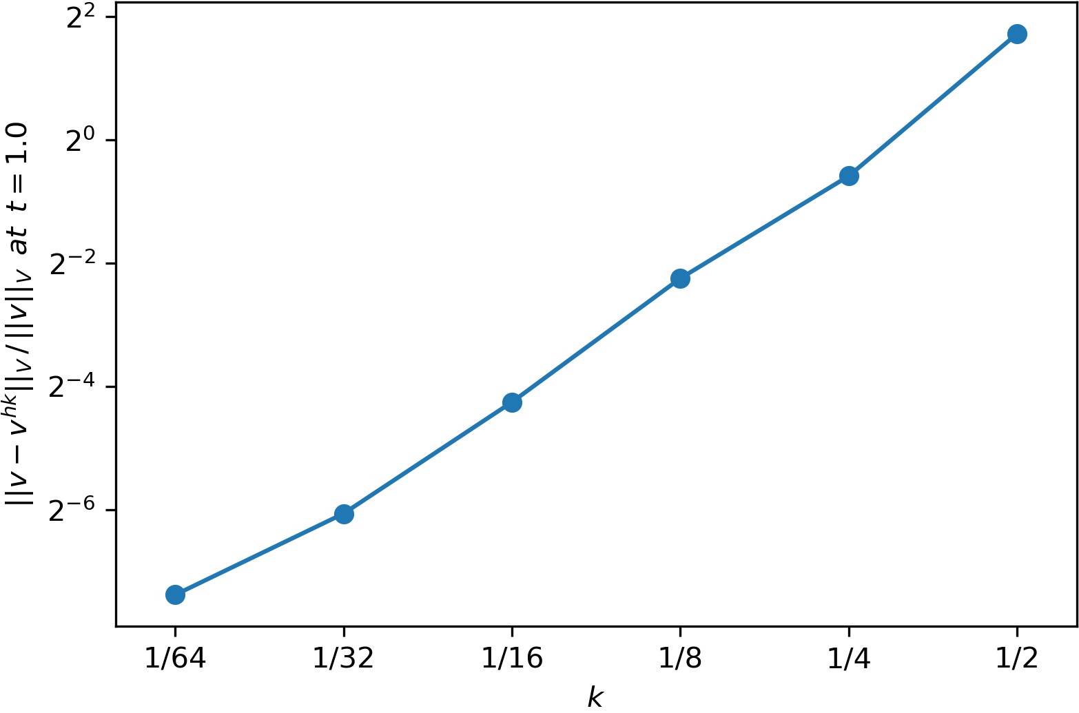
kk 1/21/2 1/41/4 1/81/8 1/161/16 1/321/32 1/641/64
‖𝒗−𝒗h​k‖V/‖𝒗‖V\|\bm{v}-\bm{v}^{hk}\|_{V}/\|\bm{v}\|_{V} 3.3088 6.6785e–1 2.1124e–1 5.2534e–2 1.4992e–2 6.0133e–3
Convergence order 2.3087 1.6606 2.0076 1.8090 1.3180
Table 1: Numerical errors for fixed h=1/256h=1/256
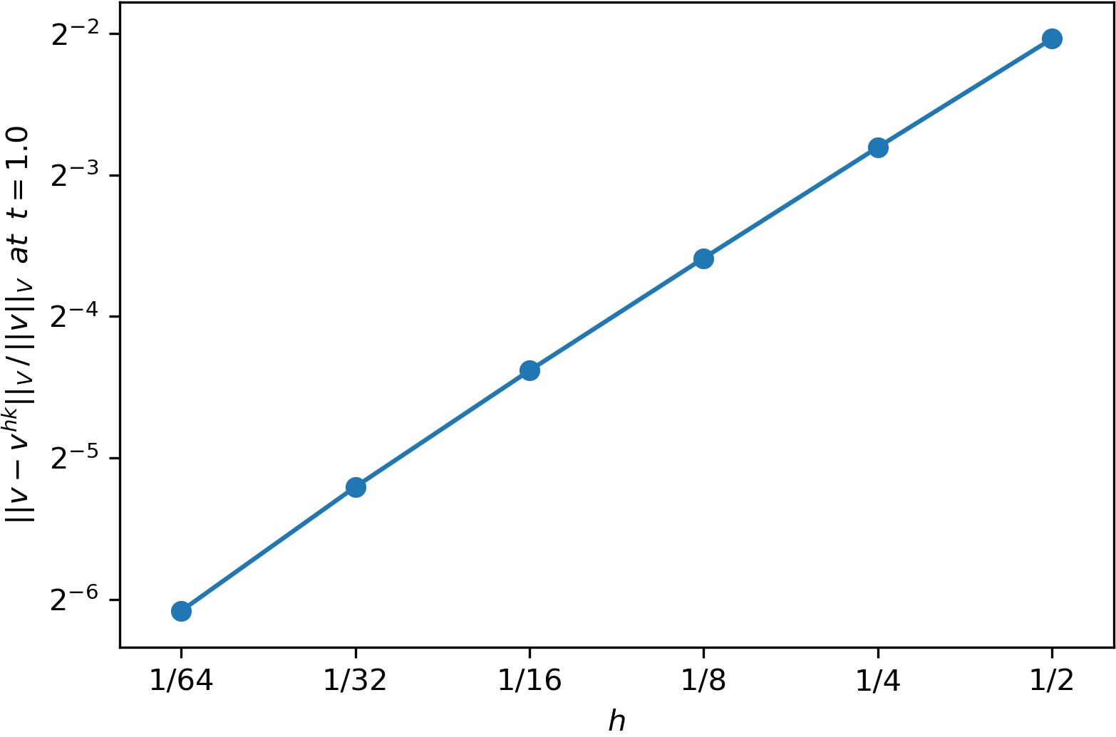
hh 1/21/2 1/41/4 1/81/8 1/161/16 1/321/32 1/641/64
‖𝒗−𝒗h​k‖V/‖𝒗‖V\|\bm{v}-\bm{v}^{hk}\|_{V}/\|\bm{v}\|_{V} 2.4390 1.4329e–1 8.3185e–2 4.7945e–2 2.7101e–2 1.4753e–2
Convergence order 0.7673 0.7845 0.7949 0.8230 0.8773
Table 2: Numerical errors for fixed k=1/256k=1/256
Refer to caption
Figure 6: Error estimate, fixed h=1/256h=1/256
Refer to caption
Figure 7: Error estimate, fixed k=1/256k=1/256

In order to illustrate the error estimate obtained in Section 3, we present the empirical convergence orders of the numerical method on the model problem. We take the following data

𝒖0​(𝒙)=(0,0),𝒙∈Ω,\displaystyle\bm{u}_{0}(\bm{x})=(0,0),\quad\bm{x}\in\Omega,
gν​(𝒙,η)={0,η∈(−∞, 0),60​η,η∈[0, 0.1),6,η∈[0.1,∞),​𝒙∈ΓC,\displaystyle g_{\nu}(\bm{x},\eta)=\left\{\begin{array}[]{ll}0,&\eta\in(-\infty,\,0),\\ 60\,\eta,&\eta\in[0,\,0.1),\\ 6,&\eta\in[0.1,\infty),\\ \end{array}\right.\bm{x}\in\Gamma_{C},
gτ​(𝒙,η)={0,η∈(−∞, 0),120​η,η∈[0, 0.1),12,η∈[0.1,∞),​𝒙∈ΓC,\displaystyle g_{\tau}(\bm{x},\eta)=\left\{\begin{array}[]{ll}0,&\eta\in(-\infty,\,0),\\ 120\,\eta,&\eta\in[0,\,0.1),\\ 12,&\eta\in[0.1,\infty),\\ \end{array}\right.\bm{x}\in\Gamma_{C},
jτ​(𝒙,𝝃)=‖𝝃‖,𝝃∈ℝ2,𝒙∈ΓC,\displaystyle j_{\tau}(\bm{x},\bm{\xi})=\|\bm{\xi}\|,\quad\bm{\xi}\in\mathbb{R}^{2},\ \bm{x}\in\Gamma_{C},
𝒇N​(𝒙,t)=(−0.2,−0.2),𝒙∈Ω,t∈[0,T],\displaystyle\bm{f}_{N}(\bm{x},t)=(-0.2,-0.2),\quad\bm{x}\in\Omega,\ t\in[0,T],
𝒇0​(𝒙,t)=(−1,−0.4),𝒙∈Ω,t∈[0,T].\displaystyle\bm{f}_{0}(\bm{x},t)=(-1,-0.4),\quad\bm{x}\in\Omega,\ t\in[0,T].

We have ‖𝒗‖V≐0.06738\|\bm{v}\|_{V}\doteq 0.06738. We present a comparison of numerical errors ‖𝒗−𝒗h​k‖V\|\bm{v}-\bm{v}^{hk}\|_{V} computed for a sequence of solutions to discretized problems. We use a uniform discretization of the problem domain and time interval according to the spatial discretization parameter hh and the time step size kk, respectively. The boundary ΓC\Gamma_{C} of Ω\Omega is divided into 1/h1/h equal parts. The numerical solution corresponding to h=1/256h=1/256 and k=1/256k=1/256 is taken as the “exact” solution 𝒗\bm{v}.

For the first experiment, we fix h=1/256h=1/256 and start with k=1/2k=1/2, which is successively halved. The results are presented in Table 1 and Figure 7, where the dependence of the relative error estimates ‖𝒗−𝒗h​k‖V/‖𝒗‖V\|\bm{v}-\bm{v}^{hk}\|_{V}/\|\bm{v}\|_{V} with respect to kk are plotted on a log-log scale. A first order convergence can be observed for the numerical solutions of the displacement.

For the second experiment, we fix k=1/256k=1/256 and start with h=1/2h=1/2, which is also successively halved. The results are presented in Table 2 and Figure 7. Again, a first order convergence can be observed.

Acknowledgments
The project has received funding from the European Union’s Horizon 2020 Research and Innovation Programme under the Marie Sklodowska-Curie grant agreement no. 823731 CONMECH. It is supported by the projects financed by the Ministry of Science and Higher Education of Republic of Poland under Grants Nos. 4004/GGPJII/H2020/2018/0 and 440328/PnH2/2019.

References

  • [1] A. Bagirov, N. Karmitsa, M. M. Mäkelä, Introduction to Nonsmooth Optimization Theory, Practice and Software, Springer International Publishing, 2014.
  • [2] M. Barboteu, K. Bartosz, P. Kalita, An analytical and numerical approach to a bilateral contact problem with nonmonotone friction, International Journal of Applied Mathematics and Computer Science, 23(2) (2013), 263–276.
  • [3] M. Barboteu, W. Han, S. Migórski, On numerical approximation of a variational–hemivariational inequality modeling contact problems for locking materials, Computers and Mathematics with Applications, 77 (2018), 898-1221.
  • [4] S.C. Brenner, L.R. Scott, The Mathematical Theory of Finite Element Methods, Third Edition, Springer-Verlag, New York, 2008.
  • [5] P. G. Ciarlet, The Finite Element Method for Elliptic Problems, North Holland, Amsterdam, 1978.
  • [6] F. H. Clarke, Optimization and Nonsmooth Analysis, Wiley Interscience, New York, 1983.
  • [7] L. Fan, S. Liu, S. Gao, Generalized monotonicity and convexity of non-differentiable functions, Journal of Mathematical Analysis and Applications, 279 (2003), 276–289.
  • [8] W. Han, Numerical analysis of stationary variational-hemivariational inequalities with applications in contact mechanics, Mathematics and Mechanics of Solids, 23 (2018), 279–293.
  • [9] W. Han, S. Migórski, M. Sofonea, A class of variational-hemivariational inequalities with applications to frictional contact problems, SIAM Journal on Mathematical Analysis, 46(6) (2014), 3891–3912.
  • [10] W. Han, M. Sofonea, Quasistatic Contact Problems in Viscoelasticity and Viscoplasticity, American Mathematical Society and International Press, 2002.
  • [11] W. Han, M. Sofonea, Numerical analysis of hemivariational inequalities in contact mechanics, Acta Numerica, 28 (2019), 175–286.
  • [12] W. Han, M. Sofonea, M. Barboteu, Numerical analysis of elliptic hemivariational inequalities, SIAM Journal on Numerical Analysis, 55(2) (2017), 640–663.
  • [13] W. Han, M. Sofonea, D. Danan, Numerical analysis of stationary variational–hemivariational inequalities, Numerische Mathematik, 139(3) (2018), 563–592.
  • [14] J. Haslinger, M. Miettinen, P.D. Panagiotopoulos, Finite Element Method for Hemivariational Inequalities. Theory, Methods and Applications, Kluwer Academic Publishers, Boston, 1999.
  • [15] M. Jureczka, A. Ochal, A nonsmooth optimization approach for hemivariational inequalities with applications in Contact Mechanics, Applied Mathematics and Optimization (2019), doi.org/10.1007/s00245-019-09593-y.
  • [16] M. Jureczka, A. Ochal, Numerical analysis and simulations of contact problem with wear, Computers and Mathematics with Applications 77(11), (2018), 2980–2988.
  • [17] N. Kikuchi, J. T. Oden, Contact Problems in Elasticity: A Study of Variational Inequalities and Finite Element Methods, SIAM, Philadelphia, 1988.
  • [18] M. Miettinen, J. Haslinger, Finite element approximation of vector-valued hemivariational problems, Journal of Global Optimization, 10(1) (1997), 17–35.
  • [19] S. Migórski, A. Ochal, M. Sofonea, Nonlinear Inclusions and Hemivariational Inequalities. Models and Analysis of Contact Problems, Advances in Mechanics and Mathematics, vol. 26, Springer, 2013.
  • [20] P.D. Panagiotopoulos, Hemivariational Inequalities, Applications in Mechanics and Engineering, Springer-Verlag, 1993.
  • [21] M. Sofonea, S. Migórski, Variational-Hemivariational Inequalities with Applications, Chapman and Hall/CRC Press, Boca Raton-London, 2018.
  • [22] P. Wriggers, Computational Contact Mechanics, Wiley, Chichester, 2002.