Why case fatality ratios can be misleading: individual- and population-based mortality estimates and factors influencing them
Abstract
Different ways of calculating mortality ratios during epidemics have yielded very different results, particularly during the current COVID-19 pandemic. We formulate both a survival probability model and an associated infection duration-dependent SIR model to define individual- and population-based estimates of dynamic mortality ratios. The key parameters that affect the dynamics of the different mortality estimates are the incubation period and the time individuals were infected before confirmation of infection. We stress that none of these ratios are accurately represented by the often misinterpreted case fatality ratio (CFR), the number of deaths to date divided by the total number of confirmed infected cases to date. Using data on the recent SARS-CoV-2 outbreaks, we estimate and compare the different dynamic mortality ratios and highlight their differences. Informed by our modeling, we propose more systematic methods to determine mortality ratios during epidemic outbreaks and discuss sensitivity to confounding effects and uncertainties in the data.
Introduction
The mortality ratio is a key metric describing the severity of a viral disease Verity et al. 2020. These metrics typically change in time before converging to a constant value and can be defined in a number of ways. One commonly used metric is the (confirmed) case fatality ratio (CFR or cCFR), the total number of deaths to date, , divided by the total number of all confirmed cases to date Garske et al. 2009; Xu et al. 2020a; Wu and McGoogan 2020; Verity et al. 2020. Infection fatality ratios (IFR), the number of deaths to date divided by the number of all infecteds, have also been used Jung et al. 2020; Famulare 2020; Oke and Heneghan 2020 although the IFR requires an estimate of the number of unconfirmed infecteds.
Both the CFR and IFR have been widely estimated from aggregated population data from past outbreaks Garske et al. 2009 as well as from those of the recent SARS-CoV-2 outbreaks Verity et al. 2020; Oke and Heneghan 2020; Jung et al. 2020; Angelopoulos et al. 2020; Mizumoto and Chowell 2009; Ruan 2020; Spychalski et al. 2020. We show examples of CFR curves in Fig. 1 and in the Supplemental Information (SI). As of March 31, 2020, the global cor 2020, while CFRs in individual regions vary significantly. Clearly, this estimate would correspond to the actual mortality ratio if (i) all infecteds were tested and (ii) all remaining unresolved individuals recover. However, some infected patients will die, increasing the estimated mortality ratio over time. Despite the underestimation of this type of population-based measurement, it is still commonly being used by various health officials and is often inconsistently defined as deaths/(deaths + recovereds) even though this difference has been clearly distinguished Ghani et al. 2005.


During the severe 2003 acute respiratory syndrome (SARS) outbreak in Hong Kong, the World Health Organization (WHO) also used the aforementioned estimate to obtain a CFR of 4.5% while the final values, after resolution of infecteds, approached 17.0% Yip et al. 2005a; Yip et al. 2005b. For the ongoing SARS-CoV-2 outbreaks, analyses by WHO and many others still use the metric Spychalski et al. 2020; Mizumoto and Chowell 2009; Oke and Heneghan 2020, (see Table 1), or time-shifted variants Famulare 2020; Verity et al. 2020. Since true mortality rates are critical for assessing the risks associated with epidemic outbreaks, typical underestimations by s may lead to insufficient countermeasures and a more severe epidemic Böttcher et al. 2015; Böttcher et al. 2016.
An unambiguous definition of mortality ratio is the probability that a single, newly infected individual will eventually die of the disease. If there are sufficient individual-level or cohort data, these probabilities can be further stratified according to patient age, gender, health condition, etc. Riou et al. 2020; Verity et al. 2020. This intrinsic mortality ratio, or probability of death, should be an intrinsic property of the virus and the infected individual, depending on age, health, access to health care, etc., and ought not directly depend on the population-level dynamics of infected and recovered individuals. Thus, it can be framed as a survival probability of a single infected individual. Whether this individual infects others does not directly affect his probability of eventually dying 11 1 Of course, at the population level, if there are many deaths, medical facilities are stressed which indirectly leads to an increase in death rates..
In the Results, we derive a model describing the probability that an infected individual dies or recovers before time . Importantly, these models incorporate the duration of infection (including an incubation period) before a patient tests positive at time . However, the CFR and other mortality measures are typically reported based on population data. Do these population-based measures, including CFR, provide reasonable measures of the probability of death of an individual? Also in the Results, we describe how mortality ratios are defined within population-level models, specifically, a disease duration-structured SIR model. We will show that population-based estimates are typically not a meaningful measure of mortality, but that under simplifying assumptions, the mortality ratio , where is the number of recovereds up to time , is more closely related to the true probability of death Ghani et al. 2005. The simplest population-level mortality ratio is currently (as of March 31, 2020) cor 2020, significantly higher than the March 31, 2020 CFR estimate.
We use the same estimates for the rate parameters in our individual and population models to compute the different mortality ratios. Note that in general, both the individual mortality probability and the population-based estimates depend on the time of measurement . By critically analyzing these estimates, the CFR, and a “delayed” case fatality ratio , we illustrate and interpret the differences among these measures and discuss how changes or uncertainty in the data affect them. In the Discussion, we summarize our results and identify a correction factor to transform population-level mortality estimates into individual mortality probabilities.
| reference | CFR |
|---|---|
| Xu et al. Xu et al. 2020a; Xu et al. 2020b and Mahase Mahase 2020 | 2% |
| Wu et al. Wu and McGoogan 2020 | 0.1-1% (outside Wuhan) |
| World Health Organization Organization 2020a; Organization 2020b | 2-4% |
| Porcheddu et al. Porcheddu et al. 2020 | 2.3% (Italy and China) |
| Peeri Peeri et al. 2020 et al. | 2% |
Results
Intrinsic individual mortality rate
Consider an individual that, at the time of positive testing , had been infected for a duration . A “survival” probability density can be defined such that is the probability that the patient is still alive and infected (not recovered) at time and has been infected for a duration between and . Since is unknown, it must be estimated or averaged over some distribution. The individual survival probability evolves according to
| (1) |
where the death and recovery rates, and , depend explicitly on the duration of infection at time and implicitly on patient health and age 22 2 The timescale of infections are much smaller than the aging process. In other words, the aging process across the disease time scale is negligible and the age-dependent transport terms can be neglected.. They may also depend explicitly on time to reflect changes in clinical policy or available health care. For example, enhanced medical care may decrease the death rate , giving the individual’s intrinsic physiological processes a chance to cure the patient.
If we assume an initial condition of one individual having been infected for time at the time of confirmation, Eq. 1 can be solved using the method of characteristics (see the SI). From the solution (see the Methods) one can derive the probabilities of death and recovery by time as
| (2) |
The probability that an individual died before time , conditioned on resolution (either death or recovery), is then defined as
| (3) |
Equations (2) and (3) also depend on all other relevant patient attributes such as age, accessibility to health care, etc. In the long-time limit, when resolution has occurred (), the individual mortality ratio is simply . In order to capture the dependence of death and recovery rates on the time an individual has been infected, we propose a constant recovery rate and a piece-wise constant death rate that is not explicitly a function of time :
| (4) |
where is the incubation time during which the patient is asymptomatic, has zero death rate, but can recover by clearing the virus. In other words, some patients fully recover without ever developing serious symptoms.



For coronavirus infections, the incubation period appears to be highly variable with a mean of Lai et al. 2020. We can estimate and using individual patient data where 19 patients (outside Hubei) had been tracked from the date on which their first symptoms occurred until the disease resolved nCoV 2019 Data Working Group 2020.
Two out of 19 patients died, on average, 20.5 days after first symptoms occurred and the mean recovery time of the remaining 17 patients is 16.8 days. We show the recovery-time distribution in Fig. 2(a). Since we know that the mortality ratio in this dataset is , we can determine the dependence between and according to (or ). The constant recovery and after-incubation period death rates Keeling and Rohani 2011 are estimated to be
| (5) |
Using these numbers, the recovery and death rate functions and are plotted as functions of in Fig. 2(b). We show the evolution of at different values of in Fig. 2(c). The corresponding long-time limit is readily apparent in Fig. 2(d): for , , while when . The smaller expected mortality associated with early identification of infection arises from the remaining incubation time during which the patient has a chance to recover without possibility of death. When conditioned on testing positive at or after the incubation period, the patient immediately suffers a positive death rate, increasing his .
Finally, in order to infer (and also indirectly and ) during an outbreak, a number of statistical issues must be considered. First, if the outbreak is ongoing, there may not be sufficient long-time cohort data. Second, is unknown. Since testing typically occurs at the onset of symptoms, most positive patients will have been infected a few days earlier. The uncertainty in can be represented by a probability density for the individual. The expected mortality can then be constructed as an average over :
| (6) |
where and are the -averaged probabilities death and cure probabilities.
Some properties of the distribution can be inferred from the behavior of patients. Before symptoms arise, only very few patients will know they have been infected, seek medical care, and get their case confirmed (i.e., for ). The majority of patients will contact hospitals/doctors when they have been infected for a duration of . The distribution thus reaches its maximum near or shortly after . Since patients are most likely to test positive after experiencing symptoms, we choose a gamma distribution
| (7) |
with shape parameter and rate parameter so that the mean is equal to .
Upon using the rates in Eqs. (4) and averaging over , we derived expressions for , and which are explicitly given in the SI. Using the values in Eq. (5) we find an expected individual mortality ratio (which are subsequently plotted in Fig. 3) and its asymptotic value . Of course, it is also possible to account for more complex time-dependent forms of and Böttcher and Antulov-Fantulin 2020, but we will primarily use Eqs. (4) in our subsequent analyses.
In the next section, we define population-based estimates for mortality ratios, , and explore how they can be computed using SIR-type models. By comparing to , we gain insight into whether population-based metrics are good proxies for individual mortality ratios. We will outline the mathematical differences and additional errors that confound population-level estimates.
Infection duration-dependent SIR model
While individual mortalities can be estimated by tracking many individuals from infection to recovery or death, oftentimes, the available data are not resolved at the individual level and only total populations are given. Typically, one has the total number of cases accumulated up to time , , the number of deaths to date , and the number of cured/recovered patients to date (see Fig. 1). The CFR is simply . Note that includes unresolved cases and that . Resolution (death or recovery) of all patients, , occurs only well after the epidemic passes.
A variant of the CFR commonly used in the literature Xu et al. 2020a; Wu and McGoogan 2020 is the delayed CFR
| (8) |
where is a corresponding time lag that accounts for the duration from the day when first symptoms occurred to the day of cure/death. Many estimates of the COVID-19 mortality ratio assume that Xu et al. 2020a; Wu and McGoogan 2020 and thus underestimate the number of death cases that result from a certain number of infected individuals. Similar underestimations using have been reported in previous epidemic outbreaks of SARS Ghani et al. 2005; Yip et al. 2005a and Ebola Atkins et al. 2015.
Alternatively, a simple and interpretable population-level mortality ratio is , the death ratio of all resolved cases. To provide a concrete model for and , and hence , we will use a variant of the standard infection duration-dependent susceptible-infected-recovered (SIR)-type model described by Wu et al. 2020
| (9) |
and , where is the number of susceptibles, is density of individuals at time who have been infected for time , and is the number of recovered individuals. The rate at which an individual infected for time at time transmits the infection to a susceptible is denoted by . For simplicity, we assume only community spread and neglect immigration of infected, which can be straightforwardly incorporated Wu et al. 2020.
Note that the equation for is identical to the equation for the survival probability described by Eq. (1). It is also equivalent to McKendrick age-structured models McKendrick 1926; Chou and Greenman 2016. PMCID: PMC3894939 33 3 In both the individual model (Eq. (1)) and population models (Eq. (9)), the death and cure rates are insensitive to changes in age over the time scale of epidemic if it occurs over, say, only 1-2 years. In this limit, we consider only infection-duration dependence in the population dynamics.. Infection of susceptibles is described by the boundary condition
| (10) |
which is similar to that used in age-structured models to represent birth McKendrick 1926. Finally, we use an initial condition consistent with the infection duration density given by Eq. (7): . Note that Eq. (10) assumes that all newly infected individuals are immediately identified; i.e., these newly infected individuals start with . After solving for the infected population density, the total number of deaths and recoveries to date can be found via
| (11) |
The corresponding total number of cases in Eq. (8) is
| (12) |
In the definitions of , , and , we account for all possible death and recovery cases to date (see SI) and that newly infected individuals are immediately identified. We use these case numbers as approximations of the reported case numbers to study the evolution of mortality-ratio estimates. Mortality ratios based on these numbers underestimate the actual individual mortality (see the previous “Intrinsic individual mortality rate” subsection) since they involve individuals that have been infected for different durations , particularly recently infected individuals who have not yet died.
An alternative way to compute populations is to exclude the newly infecteds and consider only the initial cohort. The corresponding populations in this case are defined as
| (13) |
Since and do not include infecteds with , they exclude the effect of newly infected individuals, but may yield more accurate mortality-ratios as they are based on an initial cohort of individuals in the distant past. The infections that occur after contribute only to ; thus, and do not depend on the transmission rate , possible immigration of infecteds, or the number of susceptibles . Note that all the populations derived above implicitly average over for the first cohort of identified infecteds (but not subsequent infecteds). Moreover, the population density follows the same equation as provided the same is used in their respective calculations.
The two different ways of partitioning populations (Eqs. (11) and (13)) lead to two different population-level mortality ratios
| (14) |
Since the populations and , and hence , depend on disease transmission through and , we expect to carry a different interpretation from and .
In the special case in which and are constants, the time-integrated populations and factor out of and , rendering them time-independent and
| (15) |
Thus, only in the special time-homogeneous case do both population-based mortality ratios become independent of the population (and transmission ) and coincide with the individual death probability.
To illustrate the differences between , and in more general cases, we use the simple death and cure rate functions given by Eqs. (4) in solving Eqs. (1) and (9). For in Eq. (10), we account for incubation effects by neglecting transmission during the asymptomatic incubation period () and assume
| (16) |
We use the estimated basic reproductive number Lai et al. 2020 to fix . We also first assume that the susceptible population does not change appreciably before quarantine and set . Thus, we only need to solve for in Eqs. (9) and (10). We solve Eqs. (9) and (10) numerically (see the Methods section for further details) and use these numerical solutions to compute , , and (see Fig. 3(a) and (b)), which are then used in Eqs. (14) and . To determine a realistic value of the time lag , we use data on death/recovery periods of 36 tracked patients nCoV 2019 Data Working Group 2020 and find that patients recover/die, on average, after first symptoms occurred.


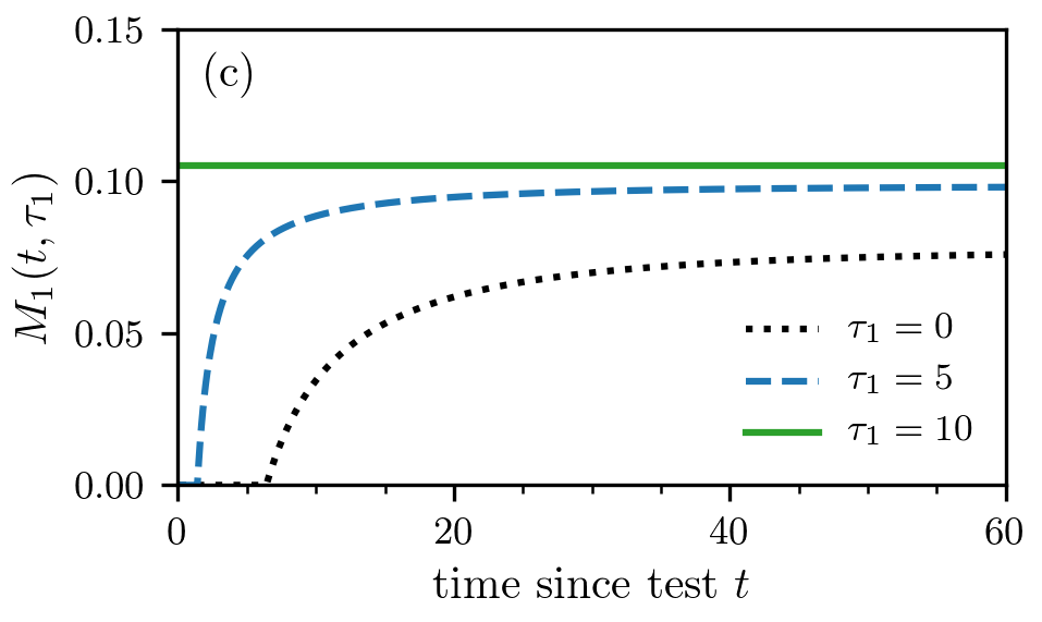
We show in Figs. 3(c) and (d) that approaches the individual mortality ratio given in the “Intrinsic individual mortality rate” subsection above. This occurs because the model for and are equivalent and we assumed the same initial distribution for both quantities. However, the population-level mortality ratios and also take into account recently infected individuals who may recover before symptoms. This difference yields different mortality ratios because newly infecteds are implicitly assumed to be detected immediately and all have . Thus, the underlying infection-time distribution is not the same as that used to compute (see the SI for further details). The mortality ratios and should not be used to quantify the individual mortality probability of individuals who tested positive. Moreover, due to evolution of the disease, , , and do not change with the same rates during an outbreak, the population-level mortality measures and reach their final steady state values only after sufficiently long times (see Fig. 3(c) and (d)).
The evolution of the mortality ratios in Fig. 3 qualitatively resembles the behavior of the mortality-ratio estimates in Fig. 1. As shown in Fig. 1, the population-based estimates for coronavirus varies, decreasing in time for China but fluctuating for Italy. These changes could result from changing practices in data collecting, or from explicitly time-inhomogeneous parameters , , and/or .
Although population-level quarantining does not directly affect the individual mortality or , it can be easily incorporated into the SIR-type population dynamics equations through changes in . For example, we have set to represent implementation of a quarantine after days of the outbreak. After days, no new infections occur and the estimates and start converging immediately towards their steady-state values (see Fig. 3(d)). Since the number of deaths decreases after the implementation of quarantine measures, the delayed is first decreasing until . For , the measures no new cases and is thus equal to the CFR.
Discussion and Summary


During an epidemic, it is important to assess the severity of the disease by estimating its mortality and other disease characteristics. Assuming accurate data, the often-used CFR typically underestimates the true, final death ratio. For example, during the SARS outbreaks in Hong Kong, the WHO first estimated the fatality rate to 2.5% (March 30, 2003) whereas the final estimates reached values of about 17.0% (June 30, 2003) (see Fig. 4(a)) Yip et al. 2005b. Standard metrics like the CFR are seen to be easily confounded by and sensitive to uncertainty in intrinsic disease parameters such as the incubation period and the time a patient had been infected before clinical confirmation of infection. For the recent COVID-19 outbreaks, CFR-based measures may still provide reasonable estimates of the actual mortality across different age classes due to a counter-acting error in the numbers of unreported mild-symptom cases.
Here, we stress that more mechanistically meaningful and interpretable metrics can be defined and, as easily, estimated from population data as CFRs. Our proposed mortality ratios for viral epidemics are defined in terms of (i) individual survival probabilities and (ii) population ratios using numbers of deaths and recovered individuals. Both of these measures are based on the within-host evolution of the disease, and in the case of , the population-level transmission dynamics.
Among the metrics we describe, is structurally closest to the individual mortality in that both are independent of disease transmission since new infections are not considered. Both of these mortality ratios converge after an incubation time to a value smaller than or equal to .
The most accurate estimates of can be obtained if we keep track of the fate of cohorts that were infected within a small time window in the past. By following only these individuals, one can track how many of them died as a function of time. As more cases arise, one should stratify them according to their estimated times since infection to gather improving statistics for . With the further spread of SARS-CoV-2 in different countries, data on more individual cases of death and recovery can be more easily stratified according to other central factors in COVID-19 mortality: age, sex, health condition.
Besides accurate cohort data, for which at present there are few for coronavirus, cumulative population data has been used to estimate the mortality ratio. The population-level metrics and implicitly depend on new infections and the transmission rate . Despite this confounding factor, and approach as , where is the probability that no recovery occurred during the incubation time . Based on these results, we can establish the following connection between the different mortality ratios for initial infection times with distribution and mean :
| (17) |
According to Eq. (17), population-level mortality estimates (e.g., CFR and ) can be transformed, at least approximately, into individual mortality probabilities using the correction factor with .
Besides the mathematical differences between and , CFR, estimating and from aggregate populations implicitly incorporate a number of confounding factors that contribute to their variability. In Fig. 4(b), we plot the population-level mortality-ratio estimates against the CFR for different regions and observe large variations and very little correlation between countries Battegay et al. 2020. As of March 31, 2020, the value of in Italy is almost 45% and can increase further if the current conditions (e.g., treatment methods, age group proportion of infecteds, etc.) do not change. Differences between the mortality ratios in China and Italy (see Figs. 1(b) and (c)) might be a result of varying medical treatment strategies, different practices in data collecting (e.g., post-mortem testing), differences in the age demographics between the countries, and/or inaccuracies in reporting.
Even if the cohort initially tested was only a fraction of the total infected population, tracking or of this cohort still provides an accurate estimation of the mortality rate. However, underreporting newly infecteds can confound CFR and . Current estimates show that only a minority of SARS-CoV-2 infections are reported (e.g., in China before January 23, 2020) Li et al. 2020. At early times (Fig. S2(a)) most patients, tested or untested, have not resolved. A reported/tested fraction would not directly affect the CFRs or mortality ratios if the unreported/untested individuals die and recover in the same proportion as the tested infecteds (Fig. S2(b)). Undertesting would overestimate the true and infection fatality ratio (IFR) if untested (presumably mildly or asymptomatic infected) individuals are less likely to die than the tested infecteds (Fig. S2(c)). If untested infecteds do not die at all, the true long-time mortality (see the SI). In the less likely scenario in which untested individuals do not receive medical care and hence die at a faster rate than tested patients (see Fig. S2(d)), and CFR based on the tested fraction would underestimate the true long-time mortality and IFR, respectively.
Besides underreporting, the delay in transmission after becoming infected will also affect . Although we have assumed that transmission occurs only after the incubation period when symptoms arise, there is evidence of asymptomatic transmission of coronavirus Rothe et al. 2020; Li et al. 2020. Asymptomatic transmission can be modeled by setting even for . An undelayed transmission in a no-quarantine scenario causes relatively more new infecteds who have not had the chance to die yet, leading to a smaller mortality ratio . Within our SIR model, delaying transmission reduces the number of infected individuals and deaths at any given time but increases the measured mortality ratio . Without quarantine, the asymptotic values and will also change as a result of changing the transmission latency period, as shown in the SI. With perfect quarantining, the asymptote is eventually determined by a cohort that does not include new infections and is thus independent of the transmission delay.
In this work, we have explicitly defined a number of interpretable mathematical metrics that represent the probability of dying from a disease By rigorously defining these metrics, we are able to reveal the inherent assumptions and factors that affect their estimation. Within survival probability and SIR-type models, we explicitly illustrate how physiologically important parameters such as incubation time, death rate, cure rate, and transmissibility influence the temporal evolution and asymptotic values of mortality ratios. We also discussed how statistical factors such as time of testing after infection () and testing ratio () affect our estimates. In practice, the mortality ratios and may provide good estimates of mortality of patients who have tested positive. In addition to our metrics and mathematical models, we emphasize the importance of curating individual cohort data. These data are more directly related to the probability of death and are subject to the fewest confounding factors and statistical uncertainty.
Data availability
The datasets that we used in this study are stored in the publicly accessible repositories of Refs. nCoV 2019 Data Working Group 2020; cor 2020; Dong et al. 2020.
Acknowledgements
LB acknowledges financial support from the SNF Early Postdoc.Mobility fellowship on “Multispecies interacting stochastic systems in biology”. The authors also acknowledge financial support from the Army Research Office (W911NF-18-1-0345), the NIH (R01HL146552), and the National Science Foundation (DMS-1814364).
Competing interests
The authors declare no competing interests.
Author contributions
LB and TC developed the analyses and wrote the manuscript. LB and MX analyzed data, performed numerical computations, and edited the manuscript.
References
- Verity et al. (2020) Robert Verity, Lucy C. Okell, Ilaria Dorigatti, Peter Winskill, Charles Whittaker, Natsuko Imai, Gina Cuomo-Dannenburg, Hayley Thompson, Patrick G. T. Walker, Han Fu, Amy Dighe, Jamie T Griffin, Marc Baguelin, Sangeeta Bhatia, Adhiratha Boonyasiri, Anne Cori, Zulma Cucunubá, Rich FitzJohn, Katy Gaythorpe, Will Green, Arran Hamlet, Wes Hinsley, Daniel Laydon, Gemma Nedjati-Gilani, Prof Steven Riley, Sabine van Elsland, Erik Volz, Haowei Wang, Yuanrong Wang, Xiaoyue Xi, Christl A. Donnelly, Azra C. Ghani, and Neil M. Ferguson, “Estimates of the severity of coronavirus disease 2019: a model-based analysis,” The Lancet Infectious Diseases (2020), 10.1016/S1473-3099(20)30243-7.
- Garske et al. (2009) Tini Garske, Judith Legrand, Christl A Donnelly, Helen Ward, Simon Cauchemez, Christophe Fraser, Neil M Ferguson, and Azra C Ghani, “Assessing the severity of the novel influenza A/H1N1 pandemic,” BMJ 339 (2009), 10.1136/bmj.b2840, https://www.bmj.com/content .
- Xu et al. (2020a) Zhe Xu, Lei Shi, Yijin Wang, Jiyuan Zhang, Lei Huang, Chao Zhang, Shuhong Liu, Peng Zhao, Hongxia Liu, Li Zhu, et al., “Pathological findings of COVID-19 associated with acute respiratory distress syndrome,” Lancet Resp. Med. (2020a).
- Wu and McGoogan (2020) Zunyou Wu and Jennifer M McGoogan, “Characteristics of and Important Lessons From the Coronavirus Disease 2019 (COVID-19) Outbreak in China: Summary of a Report of 72314 Cases From the Chinese Center for Disease Control and Prevention,” JAMA (2020).
- Jung et al. (2020) Sung-mok Jung, Andrei R. Akhmetzhanov, Katsuma Hayashi, Natalie M. Linton, Yichi Yang, Baoyin Yuan, Tetsuro Kobayashi, Ryo Kinoshita, and Hiroshi Nishiura, “Real-Time Estimation of the Risk of Death from Novel Coronavirus (COVID-19) Infection: Inference Using Exported Cases,” Journal of Clinical Medicine 9 (2020), 10.3390/jcm9020523.
- Famulare (2020) Mike Famulare, “2019-nCoV: preliminary estimates of the confirmed-case-fatality-ratio and infection-fatality-ratio, and initial pandemic risk assessment,” https://institutefordiseasemodeling.github.io/nCoV-public/analyses/first_adjusted_mortality_estimates_and_risk_assessment/2019-nCoV-preliminary_age_and_time_adjusted_mortality_rates_and_pandemic_risk_assessment.html (2020), accessed: 2020-03-31.
- Oke and Heneghan (2020) Jason Oke and Carl Heneghan, “Global Covid-19 Case Fatality Rates: Oxford COVID-19 Evidence Service,” (2020), accessed: 2020-03-27.
- Angelopoulos et al. (2020) Anastasios Nikolas Angelopoulos, Reese Pathak, Rohit Varma, and Michael I. Jordan, “Identifying and Correcting Bias from Time- and Severity- Dependent Reporting Rates in the Estimation of the COVID-19 Case Fatality Rate,” arXiv:2003.08592v2 (2020).
- Mizumoto and Chowell (2009) K. Mizumoto and G. Chowell, “Estimating risk for death from 2019 novel coronavirus disease, China, January-February 2020,” Emerging Infectious Diseases (2009), 10.3201/eid2606.200233.
- Ruan (2020) Shigui Ruan, “Likelihood of survival of coronavirus disease 2019,” The Lancet Infectious Diseases (2020), https://doi.org/10.1016/S1473-3099(20)30257-7.
- Spychalski et al. (2020) Piotr Spychalski, Agata Błażyńska-Spychalska, and Jarek Kobiela, “Estimating case fatality rates of covid-19,” The Lancet Infectious Diseases (2020), https://doi.org/10.1016/S1473-3099(20)30246-2.
- cor (2020) “COVID-19 statistics,” https://www.worldometers.info/coronavirus/ (2020), accessed: 2020-02-26.
- Ghani et al. (2005) AC Ghani, CA Donnelly, DR Cox, JT Griffin, C Fraser, TH Lam, LM Ho, WS Chan, RM Anderson, AJ Hedley, et al., “Methods for estimating the case fatality ratio for a novel, emerging infectious disease,” Am. J. Epidemiology 162, 479–486 (2005).
- Dong et al. (2020) Ensheng Dong, Hongru Du, and Lauren Gardner, “An interactive web-based dashboard to track COVID-19 in real time,” The Lancet Infectious Diseases (2020).
- Yip et al. (2005a) Paul SF Yip, KF Lam, Eric HY Lau, Pui-Hing Chau, Kenneth W Tsang, and Anne Chao, “A comparison study of realtime fatality rates: severe acute respiratory syndrome in Hong Kong, Singapore, Taiwan, Toronto and Beijing, China,” J. Roy. Stat. Soc. A 168, 233–243 (2005a).
- Yip et al. (2005b) Paul SF Yip, Eric HY Lau, KF Lam, and Richard M Huggins, “A chain multinomial model for estimating the real-time fatality rate of a disease, with an application to severe acute respiratory syndrome,” Am. J. Epidemiol. 161, 700–706 (2005b).
- Böttcher et al. (2015) Lucas Böttcher, Olivia Woolley-Meza, Nuno AM Araújo, Hans J Herrmann, and Dirk Helbing, “Disease-induced resource constraints can trigger explosive epidemics,” Sci. Rep. 5, 1–11 (2015).
- Böttcher et al. (2016) Lucas Böttcher, Olivia Woolley-Meza, Eric Goles, Dirk Helbing, and Hans J Herrmann, “Connectivity disruption sparks explosive epidemic spreading,” Phys. Rev. E 93, 042315 (2016).
- Riou et al. (2020) Julien Riou, Anthony Hauser, Michel J Counotte, and Christian L Althaus, “Adjusted age-specific case fatality ratio during the COVID-19 epidemic in Hubei, China, January and February 2020,” medRxiv (2020), 10.1101/2020.03.04.20031104.
- (20) Of course, at the population level, if there are many deaths, medical facilities are stressed which indirectly leads to an increase in death rates.
- Xu et al. (2020b) Zhou Xu, Shu Li, Shen Tian, Hao Li, and Ling-quan Kong, “Full spectrum of covid-19 severity still being depicted,” The Lancet (2020b).
- Mahase (2020) Elisabeth Mahase, “Coronavirus: COVID-19 has killed more people than SARS and MERS combined, despite lower case fatality rate,” (2020).
- Organization (2020a) World Health Organization, “WHO Director-General’s opening remarks at the media briefing on COVID-19 - 24 February 2020,” https://www.who.int/dg/speeches/detail/who-director-general-s-opening-remarks-at-the-media-briefing-on-covid-19---24-february-2020 (2020a), accessed: 2020-02-28.
- Organization (2020b) World Health Organization, “WHO Director-General’s opening remarks at the media briefing on COVID-19 - 3 March 2020,” https://www.who.int/dg/speeches/detail/who-director-general-s-opening-remarks-at-the-media-briefing-on-covid-19---3-march-2020 (2020b), accessed: 2020-03-05.
- Porcheddu et al. (2020) R. Porcheddu, C. Serra, D. Kelvin, N. Kelvin, and S. Rubino, “Similarity in Case Fatality Rates (CFR) of COVID-19/SARS-COV-2 in Italy and China,” The Journal of Infection in Developing Countries 14, 125–128 (2020).
- Peeri et al. (2020) Noah C Peeri, Nistha Shrestha, Md Siddikur Rahman, Rafdzah Zaki, Zhengqi Tan, Saana Bibi, Mahdi Baghbanzadeh, Nasrin Aghamohammadi, Wenyi Zhang, and Ubydul Haque, “The SARS, MERS and novel coronavirus (COVID-19) epidemics, the newest and biggest global health threats: what lessons have we learned?” International Journal of Epidemiology (2020), 10.1093/ije/dyaa033.
- (27) The timescale of infections are much smaller than the aging process. In other words, the aging process across the disease time scale is negligible and the age-dependent transport terms can be neglected.
- nCoV 2019 Data Working Group (2020) nCoV 2019 Data Working Group, “Epidemiological Data from the nCoV-2019 Outbreak: Early Descriptions from Publicly Available Data,” http://virological.org/t/epidemiological-data-from-the-ncov-2019-outbreak-early-descriptions-from-publicly-available-data/337 (2020), accessed: 2020-02-26.
- Lai et al. (2020) Chih-Cheng Lai, Tzu-Ping Shih, Wen-Chien Ko, Hung-Jen Tang, and Po-Ren Hsueh, “Severe acute respiratory syndrome coronavirus 2 (SARS-CoV-2) and corona virus disease-2019 (COVID-19): the epidemic and the challenges,” Int. J. Antimicrob. Agents , 105924 (2020).
- Keeling and Rohani (2011) Matt J Keeling and Pejman Rohani, Modeling infectious diseases in humans and animals (Princeton University Press, 2011).
- Böttcher and Antulov-Fantulin (2020) Lucas Böttcher and Nino Antulov-Fantulin, “Unifying susceptible-infected-recovered processes on networks,” arXiv preprint arXiv:2002.11765 (2020).
- Atkins et al. (2015) Katherine E Atkins, Natasha S Wenzel, Martial Ndeffo-Mbah, Frederick L Altice, Jeffrey P Townsend, and Alison P Galvani, “Under-reporting and case fatality estimates for emerging epidemics,” BMJ 350, h1115 (2015).
- Wu et al. (2020) Joseph T. Wu, Kathy Leung, Mary Bushman, Nishant Kishore, Rene Niehus, Pablo M. de Salazar, Benjamin J. Cowling, Marc Lipsitch, and Gabriel M. Leung, “Estimating clinical severity of COVID-19 from the transmission dynamics in Wuhan, China,” Nature Medicine (2020), 10.1038/s41591-020-0822-7.
- McKendrick (1926) A. G. McKendrick, “Applications of mathematics to medical problems,” Proc. Edinburgh Math. Soc. 44, 98–130 (1926).
- Chou and Greenman (2016. PMCID: PMC3894939) T. Chou and C. D. Greenman, “A Hierarchical Kinetic Theory of Birth, Death and Fission in Age-Structured Interacting Populations,” Journal of Statistical Physics 164, 49–76 (2016. PMCID: PMC3894939).
- (36) In both the individual model (Eq. (1)) and population models (Eq. (9)), the death and cure rates are insensitive to changes in age over the time scale of epidemic if it occurs over, say, only 1-2 years. In this limit, we consider only infection-duration dependence in the population dynamics.
- Organization (2020c) World Health Organization, “Cumulative Number of Reported Probable Cases of Severe Acute Respiratory Syndrome (SARS),” https://www.who.int/csr/sars/country/en/ (2020c), accessed: 2020-03-30.
- Battegay et al. (2020) Manuel Battegay, Richard Kuehl, Sarah Tschudin-Sutter, Hans H Hirsch, Andreas F Widmer, and Richard A Neher, “2019-novel Coronavirus (2019-nCoV): estimating the case fatality rate–a word of caution,” Swiss Medical Weekly 150 (2020).
- Li et al. (2020) Ruiyun Li, Sen Pei, Bin Chen, Yimeng Song, Tao Zhang, Wan Yang, and Jeffrey Shaman, “Substantial undocumented infection facilitates the rapid dissemination of novel coronavirus (SARS-CoV2),” Science (2020).
- Rothe et al. (2020) Camilla Rothe, Mirjam Schunk, Peter Sothmann, Gisela Bretzel, Guenter Froeschl, Claudia Wallrauch, Thorbjörn Zimmer, Verena Thiel, Christian Janke, Wolfgang Guggemos, Michael Seilmaier, Christian Drosten, Patrick Vollmar, Katrin Zwirglmaier, Sabine Zange, Roman Wölfel, and Michael Hoelscher, “Transmission of 2019-nCoV Infection from an Asymptomatic Contact in Germany,” New England Journal of Medicine 382, 970–971 (2020).
- Press et al. (2007) W. H. Press, S. A. Teukolsky, W. T. Vetterling, and B. P. Flannery, Numerical Recipes: The Art of Scientific Computing (Cambridge University Press, 2007).
Methods
Numerical scheme
To numerically solve Eqs. (9) and (10), we use a uniform discretization . A backward difference operator is used to approximate and a predictor-corrector Euler scheme is used to advance time Press et al. 2007. Setting the cut-offs and , the resulting discretized equations for the full SIR model are
| (18) | ||||
where is the initial predicted guess, and the last term proportional to encodes the boundary condition Eq. (10). Note that we use to indicate the numerical evaluation of . Quadrature methods such as Simpson’s rule and the trapezoidal rule can be used to approximate the integral more efficiently.
The total deaths, recovereds, and infecteds at time are found by
with analogous expressions for and . To obtain a stable integration scheme, the time steps and have to satisfy . In all of our numerical computations, we thus set , and . In the SI, we show additional plots of the magnitude of in the plane.
Solutions for -averaged probabilities
Using the method of characteristics, we find the formal solution to Eq. (1):
| (19) |
which can be used to construct the death and cure probabilities
| (20) |
If we now invoke the functional forms of and given in Eq. (4), we find explicitly
| (21) |
and
| (22) |
Finally, we can also find the -averaged probabilities for by weighting over . For example,
These solutions hold for the different regions shown in the phase plot of Fig. 5 and are equivalent to those for . Corresponding expressions for and can be found and used to construct .


Fig. 6(a) shows the magnitude of in the plane when we set constant (so that the first equation in Eq. (18) does not apply) such that /day. In this case, the epidemic continues to grow in time, but the mortality rates nonetheless converge as . In Fig. 6(b), we set for to model strict quarantining after days. We observe no new infections after the onset of strict quarantine measures. In both cases (quarantine and no quarantine), we use (see Eq. (7) in the main text) to describe the initial distribution of infection times . As time progresses, more of the distribution of moves towards smaller values until quarantine measures take effect (see Fig. 6(c) and (d)).
Supplementary Information
Additional examples of mortality-ratio evolutions


In Fig. S1, we show additional examples of mortality-ratio estimates for Iran, South Korea, Spain, Germany, Switzerland, and the United Kingdom. As in Fig. 1 in the main text, we observe that, by definition, the population-based mortality ratio is significantly larger than the corresponding CFR in all cases.
Effects of undertesting
Note that in the SIR equations determines the dynamics of the actual infected population. However, (i) typically only a fraction of the total number of infecteds might be tested and confirmed positive and (ii) the testing of newly infecteds may also be delayed by a distribution .
If positive tests represent only a fraction of the total infected population, and the confirmation of newly infecteds occurs immediately, the known infected density is given by where is the true total infected population. If testing of newly infecteds occurs after a distribution of infection times, .
In our development of and in the manuscript, we assumed the entire infected population was tested and confirmed. Thus, and were computed using and more accurately represent the mortality ratios of the population conditioned on being tested positive.

To estimate the mortality ratio of the population conditioned simply on being infected, we have to estimate the larger number of recovereds that went untested. For the most likely scenario in which untested infecteds have negligible death rate, as shown in Fig. S2(c), we can employ the SIR model without death for the untested pool of infecteds,
| (S1) |
where , the total density of infecteds, and the production of tested and untested infecteds follow the boundary conditions
| (S2) |
Here, we have assumed that testing occurs only for the infected who can die. In this scenario, the IFR, or the true CFR of all infecteds, is then , where in analogy to Eqs. (11) and (12),
| (S3) |
and
| (S4) |
The true mortality ratio is also straightforwardly defined by, for example,
| (S5) |
where
| (S6) |
with analogous expressions for , , and . At long times, after resolution of all infecteds, the untested recovered population is
| (S7) |
which yields the asymptotic true ratio as described in the Discussion and Summary. In this simple rescaling to account for untested populations, we have assumed that all deaths come from the tested pool and that the recovery rate is the same in the tested and untested pools.
Influence of different transmission rates
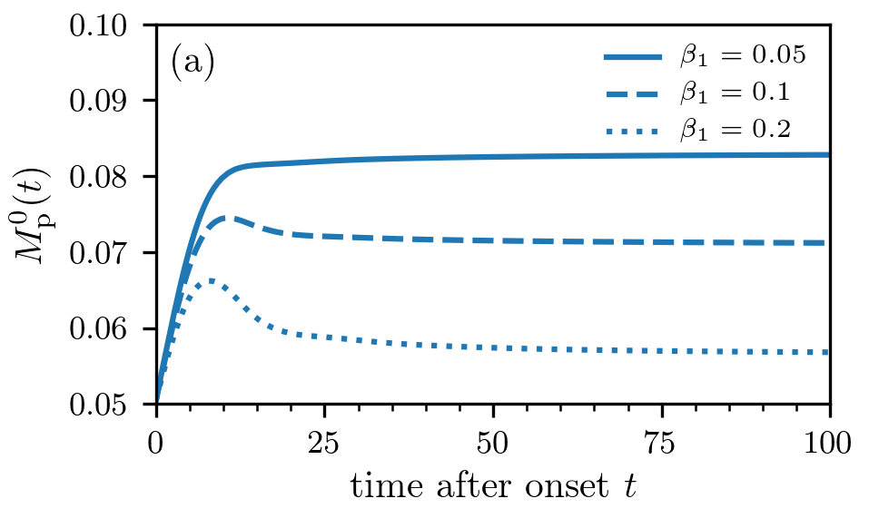
In Fig. 3 of the main text, we observe that the population-level mortality ratio approaches a plateau during the initial exponential growth phase of an epidemic (i.e., for ). If the number of new infections decreases (e.g., due to quarantine measures), starts growing until it reaches its asymptotic value . Interestingly, the pre-asymptotic values of are smaller for larger infection rates (see Fig. S3(a)). This counter-intuitive effect arises because larger values of generate relatively larger numbers of new infected which have a lower chance of dying before (see Eq. (4) in the main text).
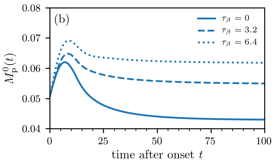
A similar effect occurs for non-delayed transmission (i.e., ). As the transmission delay decreases, more secondary cases will result from one infection, leading to smaller values of in the initial exponential growth phase of an epidemic (see Fig. S3(b)).