跳到论文正文
W Papers独立论文阅读器 arXiv:2003.11965 论文正文 计算阅读时间 · 0%
引用这篇论文根据当前论文元数据生成,正式投稿前建议核对。


License: arXiv.org perpetual non-exclusive license
arXiv:2003.11965v2 [math.AP] 27 Mar 2020

Surface homogenization of an array of Helmholtz resonators for a viscoacoustic model using two-scale convergence

Kersten Schmidta, Adrien Semina

aa: Technische Universität Darmstadt, Fachbereich Mathematik, AG Numerik und Wissenschaftliches Rechnen, Dolivostrasse 15, 64293 Darmstadt,Germany

Corresponding author: Kersten Schmidt, Technische Universität Darmstadt, Fachbereich Mathematik, AG Numerik und Wissenschaftliches Rechnen, Dolivostrasse 15, 64293 Darmstadt,Germany
E-mail: kschmidt@mathematik.tu-darmstadt.de

Keywords
asymptotic analysis; periodic surface homogenization; singular asymptotic expansions; stress intensity factor.

AMS Subject Classification 32S05, 35C20, 35J05, 35J20, 41A60, 65D15

Abstract

We derive the weak limit of a linear viscoacoustic model in an acoustic liner that is a chamber connected to a periodic repetition of elongated chambers – the Helmholtz resonators. As model we consider the time-harmonic and linearized compressible Navier-Stokes equations for the acoustic velocity and pressure. Following the approach in Schmidt et al., J. Math. Ind 8:15, 2018 for the viscoacoustic transmission problem of multiperforated plates the viscosity is scaled as δ4\delta^{4} with the period δ\delta of the array of chambers and the size of the necks as well as the wall thickness like δ2\delta^{2} such that the viscous boundary layers are of the order of the size of the necks. Applying the method of two-scale convergence we obtain with a stability assumption in the limit δ→0\delta\to 0 that the acoustic pressure fulfills the Helmholz equation with impedance boundary conditions. These boundary conditions depend on the frequency, the length of the resonators and through the effective Rayleigh conductivity – that can be computed numerically – on the shape of their necks. We compare the limit model to semi-analytical models in the literature.

1 Introduction

The noise emission from aircraft gas turbines, car engines and several other industrial applications is a matter of high concern. Its reduction is of major public interest since it affects health and life of the community. This noise reduction is also of major industrial interest. Especially, nowadays combustion processes create acoustic sources of higher intensity in aircraft engines, which in their turn create acoustic instabilities around particular frequencies and may even harm the live time of the gas turbine. Engineers study liners, which are perforated wall segments, that are able to suppress thermo-acoustic instabilities and can provide a substantial amount of acoustic damping. An important type of acounstic liner for aero-engine inlet and exhaust ducts constitues of a array of small cells called Helmholtz resonators. Each of the Helmholtz resonators – the name goes back to H. Helmholtz[19] consists of a rigid chamber filled with air that is connected to the surrounding by a hole of a perforated plate, that is called orifice or even neck. When excited with a fluctuating external pressure, that comes e. g., from the combusion process, the mass of the air inside and around the orifice moves agains the large volume of compressible air inside the cavity, while viscous effects cause dissipation of energy. This can be modeled as a mass-spring-damping system. The damping of this system is relatively small except for frequencies close to the resonance frequencies of the liner where it becomes considerably large. The resonance frequencies and damping properties depend mainly on the geometrical parameters of the resonators.

For a small Helmholtz resonator the first resonance frequency – the Helmholtz resonance – can be approximated by a simple formula[19] of Helmholtz that has been justified by a mathematical analysis of the spectrum of the Laplace operator by Schweizer[49] as well as by an asymptotic analysis of the Green’s function of the Helmholtz equation[2]. It is based on the observation that the pressure is almost uniform inside the resonator and therefore the formula does not depend on the shape of the resonator, especially, if it is elongated or of compact size. The simple formula has been improved by a so-called end-correction[32, 24] of the aperture thickness. For elongated resonance chambers approximations of each resonance frequency can be obtained as solutions of a nonlinear equations using semi-analytical formulas for the behaviour of the pressure around the hole and in the chamber[36].

For an effective damping a large number of Helmholtz resonators are arrayed. Due to the high number of resonators and the involved smaller geometrical scales a direct numerical computations, e. g., with the finite element method, would be not feasible. One is therefore interested in equivalent problems in the domain above the resonators and multiperforated plate. To predict the frequency dependent damping properties of array of Helmholtz resonators impedance boundary conditions has been proposed that depend on one complex function of the frequency – the (normalized specified) acoustic impedance. First, such a semi-analytic formula for the impedance has been introduced by Guess[18] that depends again on the end-correction of the aperture thickness, to which nonlinear terms for high sound amplitudes can be added[25, 53] that are especially important close to resonance as well as terms in presence of a gracing flow[26, 43, 48]. The impedance of an array of Helmholtz resonators is also computed numerically by coupling the instationary viscous Navier-Stokes equations in frequency domain in some region around the orifice with the Euler equation away from it by Lidoine et al. [30]. A similar approach in time-domain on meshes refined close to the orifices is used in[54] where only close to the orifices viscosity is considered. However, it is not clear what is a good choice of the “viscous” region.

In this contribution, we present an asymptotic homogenization of an array of Helmholtz resonators of depth LL, of small period δ\delta and of even smaller diameter of the orifices that is of the order δ2\delta^{2} taking the viscosity scaled like δ4\delta^{4} into account. In this way the respective dominant behaviour in three different geometric scales is considered. We derive impedance boundary conditions applying the method of two-scale convergence[35, 1] to the three different scales of the problem. To justify the weak convergence to the limit the stability estimate of the δ\delta-dependent problem has to assumed. The impedance boundary conditions is expressed in terms of the effective Rayleigh conductivity of a perforated plate [46] (see [6, 5] for zero viscosity) and in terms of the reactance of the chambers that depends above all on their depths. The effective Rayleigh conductivity is the Rayleigh conductivity [38, 39] of one hole, which describes the ratio of the fluctuating volume flow through the hole to the driving pressure difference across the hole, divided by the area of one periodicity cell of the array. The effective Rayleigh conductivity depends on the geometrical parameters, especially, size and shape of the necks of the Helmholtz resonators and the distance between two resonators, as well as the physical parameters, especially the acoustic viscosities and the excitation frequency.

Asymptotic homogenization for periodic transmission problems were performed for the Stokes equation with three scales[44], with two scales for the Helmholtz equation[8], using the periodic unfolding method[31] and the method of matched asymptotic expansion[14, 12], also with impedance boundary conditions in the holes[51]. Asymptotic homogenization for locally periodic transmission problems, where microstructures has finite size, and that takes the singular behaviour at the end of the microstructure into account, was derived and justified for the Laplace equation[34, 15] and the Helmholtz equation[50].

The article is subdivided as follows. In Sec. 2 we define the model problem of the viscous acoustic equations in terms of the acoustic velocity and pressure and the equivalent impedance boundary conditions on the array of resonators for the velocity and pressure. We also give as main result the weak convergence of the velocity and the pressure to their limits that fullfill a Helmholtz problem with the derived equivalent impedance boundary condition. For this result the assumption of an a priori stability result is needed that shall be proved in a forthcoming article. Sec. 3 is dedicated to the proof of the weak convergence to a limit using two-scale convergence step by step in different asymptotic regions where finally the limit model including impedance boundary conditions is obtained. Finally, in Sec. 4, the equivalent impedance boundary conditions are studied numerically and compared with the established model of Guess[18], both locally based on the reactance and resistance curves and resonance frequencies as well as macroscopically based on the dissipation behaviour of an array of Helmholtz resonators in a duct.

2 Description of the problem and main results

2.1 Description of the problem

We consider a three-dimensional domain Ω\Omega that is open, simply connected and bounded with smooth boundary ∂Ω\partial\Omega. For the sake of simplicity we consider that Ω\Omega is included in the half-space ℝ2×ℝ+{\mathbb{R}}^{2}\times{\mathbb{R}}_{+} such that its boundary ∂Ω\partial\Omega gives a non-empty intersection with the plane {x3=0}\{x_{3}=0\}.

We consider the surface Γ\Gamma as a parallelepipedic subset of ∂Ω∩{𝐱∈ℝ3,x3=0}\partial\Omega\cap\{{\mathbf{x}}\in{\mathbb{R}}^{3},x_{3}=0\}. We extend then the domain Ω\Omega to a domain containing an array of Helmholtz resonators. We assume this array to be periodic, i. e., there exists two fixed vectors 𝐚1{\mathbf{a}}_{1} and 𝐚2{\mathbf{a}}_{2} such that the centered parallelogram 𝒜\mathcal{A} spanned by the vectors 𝐚1{\mathbf{a}}_{1} and 𝐚2{\mathbf{a}}_{2} is of area equal to 11, and there exists δ>0\delta>0 such that the set centers of apertures of resonators is given by (see Fig. 1a)

Γδ:=Γ∩(δ​𝐚1​ℤ+δ​𝐚2​ℤ).\Gamma^{\delta}:=\Gamma\cap\big(\delta{\mathbf{a}}_{1}{\mathbb{Z}}+\delta{\mathbf{a}}_{2}{\mathbb{Z}}\big). (2.1)

For simplicity, we assume that there exists L1,L2>0L_{1},L_{2}>0 with L1/L2∈ℚL_{1}/L_{2}\in{\mathbb{Q}} such that

Γ={𝐱=s1​𝐚1+s2​𝐚2with(s1,s2)∈(0,L1)×(0,L2)},\Gamma=\{{\mathbf{x}}=s_{1}{\mathbf{a}}_{1}+s_{2}{\mathbf{a}}_{2}\quad\text{with}\quad(s_{1},s_{2})\in(0,L_{1})\times(0,L_{2})\},

and δ\delta is chosen such that L1/δL_{1}/\delta and L2/δL_{2}/\delta are positive integers, i. e., the number of Helmholtz resonators is equal to L1​L2/δ2L_{1}L_{2}/\delta^{2}. To define the resonator chamber we introduce its cross section 𝒜C⊂𝒜\mathcal{A}_{C}\subset\mathcal{A} that is a two-dimensional smooth open and simply-connected domain, and two constants d0,h0>0d_{0},h_{0}>0. For (n1,n2)∈ℤ2(n_{1},n_{2})\in{\mathbb{Z}}^{2} such that 𝐱Γδ:=δ​n1​𝐚1+δ​n2​𝐚2∈Γδ{\mathbf{x}}^{\delta}_{\Gamma}:=\delta n_{1}{\mathbf{a}}_{1}+\delta n_{2}{\mathbf{a}}_{2}\in\Gamma^{\delta}, the resonator ΩHδ​(𝐱Γδ)\Omega^{\delta}_{H}({\mathbf{x}}^{\delta}_{\Gamma}) consists of a chamber part

ΩCδ​(𝐱Γδ):=𝐱Γδ+δ​𝒜C×(−L,−δ2​h0),\Omega^{\delta}_{C}({\mathbf{x}}^{\delta}_{\Gamma}):={\mathbf{x}}^{\delta}_{\Gamma}+\delta\mathcal{A}_{C}\times(-L,-\delta^{2}h_{0}), (2.2)

and a neck part

ΩNδ​(𝐱Γδ):=𝐱Γδ+δ2​ΩN\Omega^{\delta}_{N}({\mathbf{x}}^{\delta}_{\Gamma}):={\mathbf{x}}^{\delta}_{\Gamma}+\delta^{2}\Omega_{N} (2.3)

with the bounded, open and simply connected Lipschitz domain ΩN⊂ℝ2×(−h0,0)\Omega_{N}\subset{\mathbb{R}}^{2}\times(-h_{0},0) where 0∈ΩN¯0\in\overline{\Omega_{N}} and the submanifolds ∂ΩN∩ℝ2×{0}\partial\Omega_{N}\cap{\mathbb{R}}^{2}\times\{0\} and ∂ΩN∩ℝ2×{−h0}\partial\Omega_{N}\cap{\mathbb{R}}^{2}\times\{-h_{0}\} are non-empty and smooth. Moreover, we consider δ\delta such that δ⁡(∂ΩN∩ℝ2×{−h0})⊂𝒜C×{−δ​h0}\delta\left(\partial\Omega_{N}\cap{\mathbb{R}}^{2}\times\{-h_{0}\}\right)\subset\mathcal{A}_{C}\times\{-\delta h_{0}\}. A chamber and neck builds a resonator ΩHδ​(𝐱Γδ)=ΩCδ​(𝐱Γδ)∪ΩNδ​(𝐱Γδ)\Omega^{\delta}_{H}({\mathbf{x}}^{\delta}_{\Gamma})=\Omega^{\delta}_{C}({\mathbf{x}}^{\delta}_{\Gamma})\cup\Omega^{\delta}_{N}({\mathbf{x}}^{\delta}_{\Gamma}), and extending the domain Ω\Omega by the union of all resonsators we obtain the computational domain Ωδ\Omega^{\delta} whose closure is defined by

Ωδ¯:=Ω¯∪⋃𝐱Γδ∈ΓδΩHδ​(𝐱Γδ)¯.\overline{\Omega^{\delta}}:=\overline{\Omega}\cup\bigcup_{{\mathbf{x}}^{\delta}_{\Gamma}\in\Gamma^{\delta}}\overline{\Omega^{\delta}_{H}({\mathbf{x}}^{\delta}_{\Gamma})}. (2.4)

On the domain Ωδ\Omega^{\delta} we introduce the acoustic equations in the framework of Landau and Lifschitz[28] as a perturbation of the Navier-Stokes equations around a stagnant uniform fluid with mean density ρ0\rho_{0}.

δ​𝐚1\delta{\mathbf{a}}_{1}δ​𝐚2\delta{\mathbf{a}}_{2}δ​𝒜C\delta\mathcal{A}_{C}(a) δ​|𝐚1|\delta|{\mathbf{a}}_{1}|d0​δ2d_{0}\delta^{2}areaaC​δ2a_{C}\delta^{2}h0​δ2h_{0}\delta^{2}LL(b)

Figure 1: (a) Example of one resonator (square-shaped constant cross-sections) that connects through N0=1N_{0}=1 hole. (b) Representation of the array of resonators (cut along one one periodicity direction).

We consider time-harmonic velocity 𝐯δ{\mathbf{v}}^{\delta} and acoustic pressure pδp^{\delta} (the time regime is exp⁡(−i​ω​t)\exp(-\mathrm{i}\omega t), ω>0\omega>0), which are solutions of the coupled system

−iω𝐯δ+1ρ0∇pδ−ν(δ)Δ𝐯δ−ν′(δ)∇div𝐯δ\displaystyle-\mathrm{i}\omega{\mathbf{v}}^{\delta}+\tfrac{1}{\rho_{0}}\nabla p^{\delta}-\nu(\delta)\Laplace{\mathbf{v}}^{\delta}-\nu^{\prime}(\delta)\nabla\Div{\mathbf{v}}^{\delta} =𝐟,in ​Ωδ,\displaystyle={\mathbf{f}},\quad\text{in }\Omega^{\delta}, (2.5a)
−i​ω​pδ+ρ0​c2​div⁡𝐯δ\displaystyle-\mathrm{i}\omega p^{\delta}+\rho_{0}c^{2}\Div{\mathbf{v}}^{\delta} =0,in ​Ωδ,\displaystyle=0,\quad\text{in }\Omega^{\delta}, (2.5b)
𝐯δ\displaystyle{\mathbf{v}}^{\delta} =𝟎,on ​∂Ωδ,\displaystyle=\bm{0},\quad\text{on }\partial\Omega^{\delta}, (2.5c)

with the speed of sound cc, and the kinematic and secondary viscosities ν⁡(δ),ν′​(δ)>0\nu(\delta),\nu^{\prime}(\delta)>0 that we scale with the characteristic size of the holes δ2\delta^{2} as

ν⁡(δ)=ν0​δ4andν′​(δ)=ν0′​δ4,\nu(\delta)=\nu_{0}\delta^{4}\quad\text{and}\quad\nu^{\prime}(\delta)=\nu^{\prime}_{0}\delta^{4}, (2.6)

where ν0,ν0′\nu_{0},\nu_{0}^{\prime} are independent of δ\delta. In this way the thickness of the boundary layer of the acoustic velocity at the rigid wall[3, 4, 7, 23, 47] – that is of order O⁡(ν⁡(δ))O(\sqrt{\nu(\delta)}) – is of the order of characteristic size of the holes δ2\delta^{2} (see Fig. 1(b)). Moreover, the source term 𝐟{\mathbf{f}} is independent of δ\delta and compactly supported in Ω\Omega away from its boundary. Similar equations have been studied for a stagnant flow[22, 23, 28, 42] and for the case that a mean flow is present[4, 21, 22, 33, 41]. Finally, we embed the domain Ωδ\Omega^{\delta} and the associate linear Navier-Stokes problem (2.5) in a family of problems that are δ\delta-dependent.

In the following, we define the effective Rayleigh conductivity of a single hole that will be used then to define impedance boundary conditions for the limit of (𝐯δ,pδ)({\mathbf{v}}^{\delta},p^{\delta}) for δ→0\delta\to 0.

2.2 Effective Rayleigh conductivity

To relate the pressure jump on different sides of a single hole to pressure and velocity profiles and eventually the flux through the hole we consider as characteristic problem an instationary Stokes system in scaled coordinates[46]: Seek (𝖛,𝔭)∈(H01​(Ω^))3×Lloc2​(Ω^)(\bm{\mathfrak{v}},{\mathfrak{p}})\in(\mathrm{H}_{0}^{1}(\widehat{\Omega}))^{3}\times\mathrm{L}_{\textsf{loc}}^{2}(\widehat{\Omega}) solution of

−iω𝖛+1ρ0∇𝔭−ν0Δ𝖛\displaystyle-\mathrm{i}\omega\bm{\mathfrak{v}}+\tfrac{1}{\rho_{0}}\nabla{\mathfrak{p}}-\nu_{0}\Laplace\bm{\mathfrak{v}} =𝟎,\displaystyle=\bm{0}, in ​Ω^,\displaystyle\text{in }\widehat{\Omega}, (2.7)
div⁡𝖛\displaystyle\Div\bm{\mathfrak{v}} =0,\displaystyle=0, in ​Ω^,\displaystyle\text{in }\widehat{\Omega},
𝖛\displaystyle\bm{\mathfrak{v}} =𝟎,\displaystyle=\bm{0}, on ​∂Ω^,\displaystyle\text{on }\partial\widehat{\Omega},
limS→∞𝔭|Γ^±(S)\displaystyle\lim_{S\to\infty}{\mathfrak{p}}_{|\widehat{\Gamma}_{\pm}(S)} =±12,\displaystyle=\pm\tfrac{1}{2}\ ,

with the family of surfaces

Γ^+​(S)\displaystyle\widehat{\Gamma}_{+}(S) :={𝐳∈ℝ3:|𝐳|=S,z3>0},\displaystyle:=\{{\mathbf{z}}\in{\mathbb{R}}^{3}:|{\mathbf{z}}|=S,z_{3}>0\},
Γ^−​(S)\displaystyle\widehat{\Gamma}_{-}(S) :={𝐳∈ℝ3:|𝐳−(0,0,−h0)|=S,z3<−h0}\displaystyle:=\{{\mathbf{z}}\in{\mathbb{R}}^{3}:|{\mathbf{z}}-(0,0,-h_{0})|=S,z_{3}<-h_{0}\}

and the rescaled extended aperture domain Ω^:=∪S∈ℝ+Ω^(S)\widehat{\Omega}:=\cup_{S\in{\mathbb{R}}^{+}}\widehat{\Omega}(S) connecting two half-spaces (see Fig. 2(c) for illustration) where

Ω^​(S):=Ω^A\displaystyle\widehat{\Omega}(S):=\widehat{\Omega}_{A} ∪{𝐳∈ℝ3:|𝐳|​<S,z3>​0}\displaystyle\cup\{{\mathbf{z}}\in{\mathbb{R}}^{3}:|{\mathbf{z}}|<S,z_{3}>0\}
∪{𝐳∈ℝ3:|𝐳−(0,0,−h0)|<S,z3<−h0}.\displaystyle\cup\{{\mathbf{z}}\in{\mathbb{R}}^{3}:|{\mathbf{z}}-(0,0,-h_{0})|<S,z_{3}<-h_{0}\}.

Due to the scaling all other holes are moved towards infinity and canonical problem considers the dominant phenomena on the scale of one hole, that is viscosity and incompressibility of the acoustic velocity that is with the acoustic pressure non-stationary.

The well-posedness of the characteristic problem is stated in the following

Proposition 2.1.

There exists a unique solution (𝖛,𝔭)∈(H01​(Ω^))3×Lloc2​(Ω^)(\bm{\mathfrak{v}},{\mathfrak{p}})\in(\mathrm{H}_{0}^{1}(\widehat{\Omega}))^{3}\times\mathrm{L}_{\textsf{loc}}^{2}(\widehat{\Omega}) of (2.7).

Proof.

First we lift the condition for the pressure at infinity with a cut-off function

Θ⁡(𝐳)\displaystyle\Theta({\mathbf{z}}) ={12,z3>0,12+z3h0,0>z3>−h0,−12,otherwise\displaystyle=\begin{cases}\tfrac{1}{2},&z_{3}>0,\\ \tfrac{1}{2}+\frac{z_{3}}{h_{0}},&0>z_{3}>-h_{0},\\ -\tfrac{1}{2},&\text{otherwise}\end{cases}

We decompose then the pressure 𝔭{\mathfrak{p}} as 𝔭=Θ+𝔭~{\mathfrak{p}}=\Theta+\tilde{{\mathfrak{p}}} and seek 𝔭~\tilde{{\mathfrak{p}}} in the classical space L2​(Ω^)\mathrm{L}^{2}(\widehat{\Omega}). The variational formulation associated to (2.7) is: find (𝖛,𝔭~)∈(H01​(Ω^))3×L2​(Ω^)(\bm{\mathfrak{v}},\tilde{{\mathfrak{p}}})\in(\mathrm{H}_{0}^{1}(\widehat{\Omega}))^{3}\times\mathrm{L}^{2}(\widehat{\Omega}) such that for any (𝖜,𝔮)∈(H01​(Ω^))3×L2​(Ω^)(\bm{\mathfrak{w}},{\mathfrak{q}})\in(\mathrm{H}_{0}^{1}(\widehat{\Omega}))^{3}\times\mathrm{L}^{2}(\widehat{\Omega}),

a⁡(𝖛,𝖜)+b⁡(𝔭~,𝖜)\displaystyle a(\bm{\mathfrak{v}},\bm{\mathfrak{w}})+b(\tilde{{\mathfrak{p}}},\bm{\mathfrak{w}}) =ℓ⁡(𝖜),\displaystyle=\ell(\bm{\mathfrak{w}}), (2.8)
b⁡(𝔮,𝖛)\displaystyle b({\mathfrak{q}},\bm{\mathfrak{v}}) =0,\displaystyle=0,

where the sesquilinear forms aa and bb are given by

a⁡(𝖛,𝖜)\displaystyle a(\bm{\mathfrak{v}},\bm{\mathfrak{w}}) :=−iω∫Ω^𝖛⋅𝖜¯d𝐳+ν0∫Ω^∇𝖛:∇𝖜¯d𝐳,\displaystyle:=-\mathrm{i}\omega\int_{\widehat{\Omega}}\bm{\mathfrak{v}}\cdot\overline{\bm{\mathfrak{w}}}\,\text{d}{\mathbf{z}}+\nu_{0}\int_{\widehat{\Omega}}\nabla\bm{\mathfrak{v}}:\nabla\overline{\bm{\mathfrak{w}}}\,\text{d}{\mathbf{z}}, b⁡(𝔮,𝖛)\displaystyle b({\mathfrak{q}},\bm{\mathfrak{v}}) :=−1ρ0∫Ω^𝔮div𝖛¯d𝐳,\displaystyle:=-\tfrac{1}{\rho_{0}}\int_{\widehat{\Omega}}{\mathfrak{q}}\Div\overline{\bm{\mathfrak{v}}}\,\text{d}{\mathbf{z}},

and the antilinear form ℓ\ell by

ℓ⁡(𝖜):=1ρ0​∫Ω^∇Θ⋅𝖜¯​d​𝐳.\ell(\bm{\mathfrak{w}}):=\tfrac{1}{\rho_{0}}\int_{\widehat{\Omega}}\nabla\Theta\cdot\overline{\bm{\mathfrak{w}}}\,\text{d}{\mathbf{z}}\ .

The formulation (2.8) has a saddle-point structure. The sesquilinear form aa is continuous and elliptic on (H01​(Ω^))3(\mathrm{H}_{0}^{1}(\widehat{\Omega}))^{3}. The sesquilinear form bb defines a surjective operator B:(H01​(Ω))3→L2​(Ω)B:(\mathrm{H}_{0}^{1}(\Omega))^{3}\to\mathrm{L}^{2}(\Omega) by

⟨B​𝖛,𝔮⟩Ω^=b⁡(𝔮,𝖛),∀(𝖛,𝔮)∈(H01​(Ω))3×L2​(Ω),\left<B\bm{\mathfrak{v}},{\mathfrak{q}}\right>_{\widehat{\Omega}}=b({\mathfrak{q}},\bm{\mathfrak{v}}),\quad\forall(\bm{\mathfrak{v}},{\mathfrak{q}})\in(\mathrm{H}_{0}^{1}(\Omega))^{3}\times\mathrm{L}^{2}(\Omega),

with closed range.

Following the theory of saddle-point problems[11] and in view of Theorem 1.1 of the works of Brezzi[10], problem (2.8) admits a unique solution (𝖛,𝔭~)∈(H01​(Ω^))3×L2​(Ω^)(\bm{\mathfrak{v}},\tilde{{\mathfrak{p}}})\in(\mathrm{H}_{0}^{1}(\widehat{\Omega}))^{3}\times\mathrm{L}^{2}(\widehat{\Omega}), and, hence, (2.7) has a unique solution. ∎

Following the formulation of the Rayleigh conductivity KRK_{R}[38, 39] which describes the ratio of the fluctuating volume flow to the driving pressure difference, we introduce the effective Rayleigh conductivity kRk_{R}[6, 46] as

kR:=limS→∞i​ω​ρ02​(∫Γ^+​(S)𝖛⋅𝐧−∫Γ^−​(S)𝖛⋅𝐧).k_{R}:=\lim_{S\to\infty}\frac{\mathrm{i}\omega\rho_{0}}{2}\Big(\int_{\widehat{\Gamma}_{+}(S)}\bm{\mathfrak{v}}\cdot{\mathbf{n}}-\int_{\widehat{\Gamma}_{-}(S)}\bm{\mathfrak{v}}\cdot{\mathbf{n}}\Big). (2.9)
Proposition 2.2.

The above defined effective Rayleigh conductivity kRk_{R} is well defined, i. e., the integral of the normal flux of 𝖛\bm{\mathfrak{v}} on Γ^±​(S)\widehat{\Gamma}_{\pm}(S) tends to a finite, non-zero quantity as SS tends to infinity. Moreover Re⁡(kR)>0\mathrm{Re}(k_{R})>0 and Im⁡(kR)<0\mathrm{Im}(k_{R})<0.

Proof.

Taking the conjugate of (3.21a) leads to

i​ω​𝖛¯+1ρ0​∇𝐳𝔭¯−ν0​Δ𝐳​𝖛¯=𝟎.\mathrm{i}\omega\overline{\bm{\mathfrak{v}}}+\tfrac{1}{\rho_{0}}\nabla_{\mathbf{z}}\overline{{\mathfrak{p}}}-\nu_{0}\Delta_{\mathbf{z}}\overline{\bm{\mathfrak{v}}}=\bm{0}.

Multiplying this equation with 𝖛\bm{\mathfrak{v}} and integrating over the domain Ω^​(S)\widehat{\Omega}(S) leads to

i​ω​‖𝖛‖L2​(Ω^​(S))2+1ρ0​⟨∇𝐳𝔭¯,𝖛⟩Ω^​(S)−ν0​⟨Δ𝐳​𝖛¯,𝖛¯⟩Ω^​(S)=0.\mathrm{i}\omega\left\lVert\bm{\mathfrak{v}}\right\rVert_{\mathrm{L}^{2}(\widehat{\Omega}(S))}^{2}+\tfrac{1}{\rho_{0}}\left<\nabla_{\mathbf{z}}\overline{{\mathfrak{p}}},\bm{\mathfrak{v}}\right>_{\widehat{\Omega}(S)}-\nu_{0}\left<\Delta_{\mathbf{z}}\overline{\bm{\mathfrak{v}}},\overline{\bm{\mathfrak{v}}}\right>_{\widehat{\Omega}(S)}=0. (2.10)

Let us treat now the two scalar product terms using the Gauss’ theorem. Using (3.21b) leads to

⟨∇𝐳𝔭¯,𝖛⟩Ω^​(S)=⟨𝔭¯,𝖛⋅𝐧⟩∂Ω^​(S)\left<\nabla_{\mathbf{z}}\overline{{\mathfrak{p}}},\bm{\mathfrak{v}}\right>_{\widehat{\Omega}(S)}=\left<\overline{{\mathfrak{p}}},\bm{\mathfrak{v}}\cdot{\mathbf{n}}\right>_{\partial\widehat{\Omega}(S)}

Using (3.21d) (which is also valid for the conjugate complex), the definition of the effective Rayleigh conductivity stated by (2.9) and the spherical harmonic decompositions of 𝔭{\mathfrak{p}} and 𝖛\bm{\mathfrak{v}} leads to

limS→∞⟨∇𝐳𝔭¯,𝖛⟩Ω^​(S)=kRi​ω​ρ0\lim_{S\to\infty}\left<\nabla_{\mathbf{z}}\overline{{\mathfrak{p}}},\bm{\mathfrak{v}}\right>_{\widehat{\Omega}(S)}=\frac{k_{R}}{\mathrm{i}\omega\rho_{0}}

Similarly, the study of the L2\mathrm{L}^{2}-scalar product between Δ𝐳​𝖛¯\Delta_{\mathbf{z}}\overline{\bm{\mathfrak{v}}} and 𝖛\bm{\mathfrak{v}} leads to

−limS→∞⟨Δ𝐳𝖛¯,𝖛¯⟩Ω^​(S)=‖∇𝖛‖L2​(Ω^)2-\lim_{S\to\infty}\left<\Delta_{\mathbf{z}}\overline{\bm{\mathfrak{v}}},\overline{\bm{\mathfrak{v}}}\right>_{\widehat{\Omega}(S)}=\left\lVert\nabla\bm{\mathfrak{v}}\right\rVert_{\mathrm{L}^{2}(\widehat{\Omega})}^{2}

Taking then the limit in (2.10) as S→∞S\to\infty leads to

i​ω​‖𝖛‖L2​(Ω^​(S))2+ν0​‖∇𝖛‖L2​(Ω^​(S))2=−kRi​ω​ρ02=1ω​ρ02​(−Im⁡(kR)+iRe⁡(kR))\mathrm{i}\omega\left\lVert\bm{\mathfrak{v}}\right\rVert_{\mathrm{L}^{2}(\widehat{\Omega}(S))}^{2}+\nu_{0}\left\lVert\nabla\bm{\mathfrak{v}}\right\rVert_{\mathrm{L}^{2}(\widehat{\Omega}(S))}^{2}=-\frac{k_{R}}{\mathrm{i}\omega\rho_{0}^{2}}=\frac{1}{\omega\rho_{0}^{2}}\big(-\mathrm{Im}(k_{R})+\mathrm{i}\mathrm{Re}(k_{R})\big)

and therefore Re⁡(kR)>0\mathrm{Re}(k_{R})>0 and Im⁡(kR)<0\mathrm{Im}(k_{R})<0. ∎

2.3 Weak convergence to a limit problem with impedance boundary conditions

As δ\delta tends to 00, we expect that the solution (𝐯δ,pδ)({\mathbf{v}}^{\delta},p^{\delta}) tends to a finite, non-trivial limit solution (𝐯0,p0)({\mathbf{v}}_{0},p_{0}) in the half-space Ω\Omega, and we expect this limit term to be solution of an inviscid Helmholtz problem posed on Ω\Omega.

Definition 2.3 (Limit problem).

We define the limit problem (𝐯0,p0)({\mathbf{v}}_{0},p_{0}) as solution of

−iω𝐯0+1ρ0∇p0\displaystyle-\mathrm{i}\omega{\mathbf{v}}_{0}+\tfrac{1}{\rho_{0}}\nabla p_{0} =𝐟,\displaystyle={\mathbf{f}}, in ​Ω,\displaystyle\text{in }\Omega, (2.11)
−i​ω​p0+ρ0​c2​div⁡𝐯0\displaystyle-\mathrm{i}\omega p_{0}+\rho_{0}c^{2}\Div{\mathbf{v}}_{0} =0,\displaystyle=0, in Ω,\displaystyle\text{in }\Omega,
(i​c​ρ0aC​cos⁡(ω​Lc)−i​ω​ρ0kR​sin⁡(ω​Lc))​𝐯0⋅𝐧−sin⁡(ω​Lc)​p0\displaystyle\Big(\tfrac{\mathrm{i}c\rho_{0}}{a_{C}}\cos\big(\tfrac{\omega L}{c}\big)-\tfrac{\mathrm{i}\omega\rho_{0}}{k_{R}}\sin\big(\tfrac{\omega L}{c}\big)\Big){\mathbf{v}}_{0}\cdot{\mathbf{n}}-\sin\big(\tfrac{\omega L}{c}\big)p_{0} =0,\displaystyle=0, on ​Γ,\displaystyle\text{on }\Gamma,
𝐯0⋅𝐧\displaystyle{\mathbf{v}}_{0}\cdot{\mathbf{n}} =0,\displaystyle=0, on ​∂Ω∖Γ.\displaystyle\text{on }\partial\Omega\setminus\Gamma.

2​δ322\delta^{\tfrac{3}{2}}δ2​h0\delta^{2}h_{0}δ2​d0\delta^{2}d_{0}𝐱Γδ{\mathbf{x}}^{\delta}_{\Gamma}(a) Extended neck domain ΩAδ​(𝐱Γδ)\Omega^{\delta}_{A}({\mathbf{x}}^{\delta}_{\Gamma}) 2​δ−122\delta^{-\tfrac{1}{2}}h0h_{0}d0d_{0}𝟎\bm{0}(b) Rescaled extendedneck domain Ω^(2δ−1/2)\widehat{\Omega}(2\delta^{-1/2}) Γ^+​(S)\widehat{\Gamma}_{+}(S)Γ^−​(S)\widehat{\Gamma}_{-}(S)h0h_{0}d0d_{0}𝟎\bm{0}(c) Limit rescaled extendedneck domain Ω^\widehat{\Omega}

Figure 2: An extended neck domain in the original coordinates 𝐱{\mathbf{x}} (left), in rescaled coordinates 𝐳:=δ−2​(𝐱−𝐱Γδ){\mathbf{z}}:=\delta^{-2}({\mathbf{x}}-{\mathbf{x}}^{\delta}_{\Gamma}) (middle) and the limit of the latter when δ→0\delta\to 0 (right).

Note that, problem (2.11) is equivalent to a problem for the limit pressure p0∈H1​(Ω)p_{0}\in\mathrm{H}^{1}(\Omega) only, that is given by

Δ​p0+ω2c2​p0\displaystyle\Delta p_{0}+\tfrac{\omega^{2}}{c^{2}}p_{0} =ρ0​div⁡𝐟,\displaystyle=\rho_{0}\Div{\mathbf{f}}, in ​Ω,\displaystyle\text{in }\Omega, (2.12)
(cω​aCcos(ω​Lc)−1kRsin(ω​Lc))∇p0⋅𝐧−sin(ω​Lc)p0\displaystyle\Big(\tfrac{c}{\omega a_{C}}\cos\big(\tfrac{\omega L}{c}\big)-\tfrac{1}{k_{R}}\sin\big(\tfrac{\omega L}{c}\big)\Big)\nabla p_{0}\cdot{\mathbf{n}}-\sin\big(\tfrac{\omega L}{c}\big)p_{0} =0,\displaystyle=0, on ​Γ,\displaystyle\text{on }\Gamma,
∇p0⋅𝐧\displaystyle\nabla p_{0}\cdot{\mathbf{n}} =0,\displaystyle=0, on ​∂Ω∖Γ,\displaystyle\text{on }\partial\Omega\setminus\Gamma,

where 𝐯0:=iω(𝐟−1ρ0∇p0){\mathbf{v}}_{0}:=\tfrac{\mathrm{i}}{\omega}\big({\mathbf{f}}-\tfrac{1}{\rho_{0}}\nabla p_{0}\big) follows. It is also equivalent to a problem for the limit velocity 𝐯0∈H⁡(div,Ω)∩H⁡(𝐜𝐮𝐫𝐥,Ω){\mathbf{v}}_{0}\in\mathrm{H}(\Div,\Omega)\cap\mathrm{H}(\Curl,\Omega) only that is

∇div⁡𝐯0+ω2c2​𝐯0\displaystyle\nabla\Div{\mathbf{v}}_{0}+\tfrac{\omega^{2}}{c^{2}}{\mathbf{v}}_{0} =i​ωc2​𝐟,\displaystyle=\tfrac{\mathrm{i}\omega}{c^{2}}{\mathbf{f}}, in ​Ω,\displaystyle\text{in }\Omega, (2.13)
𝐜𝐮𝐫𝐥⁡𝐯0\displaystyle\Curl{\mathbf{v}}_{0} =−1i​ω​𝐜𝐮𝐫𝐥⁡𝐟,\displaystyle=-\tfrac{1}{\mathrm{i}\omega}\Curl{\mathbf{f}}, in ​Ω,\displaystyle\text{in }\Omega,
(cω​aC​cos⁡(ω​Lc)−1kR​sin⁡(ω​Lc))​𝐯0⋅𝐧\displaystyle\Big(\tfrac{c}{\omega a_{C}}\cos\big(\tfrac{\omega L}{c}\big)-\tfrac{1}{k_{R}}\sin\big(\tfrac{\omega L}{c}\big)\Big){\mathbf{v}}_{0}\cdot{\mathbf{n}}
−(c2ω2​sin⁡(ω​Lc))​div⁡𝐯0\displaystyle-\Big(\tfrac{c^{2}}{\omega^{2}}\sin\big(\tfrac{\omega L}{c}\big)\Big)\Div{\mathbf{v}}_{0} =0,\displaystyle=0, on ​Γ,\displaystyle\text{on }\Gamma,
𝐯0⋅𝐧\displaystyle{\mathbf{v}}_{0}\cdot{\mathbf{n}} =0,\displaystyle=0, on ​∂Ω∖Γ,\displaystyle\text{on }\partial\Omega\setminus\Gamma,

where p0:=−i​ρ0​c2ω​div⁡𝐯0p_{0}:=\tfrac{-\mathrm{i}\rho_{0}c^{2}}{\omega}\Div{\mathbf{v}}_{0} follows.

The nature of the boundary condition on Γ\Gamma depends on the value of sin⁡ω​Lc\sin\tfrac{\omega L}{c}

  1. 1.

    If sin⁡(ω​Lc)=0\sin\big(\tfrac{\omega L}{c}\big)=0, i. e., if ωc\tfrac{\omega}{c} corresponds to a characteristic wavelength of the one-dimensional Helmholtz problem in a domain of size LL, then the boundary condition on Γ\Gamma becomes 𝐯0⋅𝐞3=0{\mathbf{v}}_{0}\cdot{\mathbf{e}}_{3}=0, therefore 𝐯0⋅𝐧=0{\mathbf{v}}_{0}\cdot{\mathbf{n}}=0 on the whole boundary ∂Ω\partial\Omega.

  2. 2.

    A contrario, if sin⁡(ω​Lc)≠0\sin\big(\tfrac{\omega L}{c}\big)\not=0, the right-hand side does not vanish, and denoting here by 𝐧:=−𝐞3{\mathbf{n}}:=-{\mathbf{e}}_{3} the unit outward normal vector on Γ\Gamma, one gets the impedance condition

    (−i​caC​(𝐱Γ)​cot⁡(ω​Lc)+i​ωkR​(𝐱Γ))​𝐯0​(𝐱Γ)⋅𝐧+1ρ0​p0​(𝐱Γ)=0,\Big(-\tfrac{\mathrm{i}c}{a_{C}({\mathbf{x}}_{\Gamma})}\cot\big(\tfrac{\omega L}{c}\big)+\tfrac{\mathrm{i}\omega}{k_{R}({\mathbf{x}}_{\Gamma})}\Big){\mathbf{v}}_{0}({\mathbf{x}}_{\Gamma})\cdot{\mathbf{n}}+\tfrac{1}{\rho_{0}}p_{0}({\mathbf{x}}_{\Gamma})=0, (2.14)

    and this equation gives an acoustic impedance Z⁡(ω)Z(\omega) of the same nature as the one derived by Rienstra and Singh[43, Eq. (14)].

We give the existence and uniqueness result of the limit problem:

Lemma 2.4 (Existence and uniqueness of the limit problem).

Let 𝐟∈H⁡(div,Ω){\mathbf{f}}\in\mathrm{H}(\Div,\Omega). Then, the limit problem (2.11) is well-posed, i. e., admits a unique solution (𝐯0,p0)∈H⁡(div,Ω)×H1​(Ω)({\mathbf{v}}_{0},p_{0})\in\mathrm{H}(\Div,\Omega)\times\mathrm{H}^{1}(\Omega), except for frequencies ω∈Λ\omega\in\Lambda, where Λ\Lambda is a subset of π​cL​ℕ\tfrac{\pi c}{L}{\mathbb{N}}.

This lemma will be proved later in Section 3.6.

We give now the main theoretical result of this paper.

Theorem 2.5 (Weak convergence to the limit problem).

Let ω∉Λ\omega\not\in\Lambda with the set Λ\Lambda in Lemma 2.4, 𝐟∈H⁡(div,Ω){\mathbf{f}}\in\mathrm{H}(\Div,\Omega) and there exist two constants CΩ>0C_{\Omega}>0 and δ0>0\delta_{0}>0 such that for all δ∈(0,δ0)\delta\in(0,\delta_{0}) it holds for the solution (𝐯δ,pδ)({\mathbf{v}}^{\delta},p^{\delta}) of (2.5)

‖𝐯δ‖H⁡(div,Ωδ)+δ2​‖𝐜𝐮𝐫𝐥⁡𝐯δ‖L2​(Ωδ)3+‖pδ‖H1​(Ωδ)⩽CΩ.\left\lVert{\mathbf{v}}^{\delta}\right\rVert_{\mathrm{H}(\Div,\Omega^{\delta})}+\delta^{2}\left\lVert\Curl{\mathbf{v}}^{\delta}\right\rVert_{\mathrm{L}^{2}(\Omega^{\delta})^{3}}+\left\lVert p^{\delta}\right\rVert_{\mathrm{H}^{1}(\Omega^{\delta})}\leqslant C_{\Omega}. (2.15)

Then (𝐯δ,pδ)({\mathbf{v}}^{\delta},p^{\delta}) converges weakly in H⁡(div,Ω)×H1​(Ω)\mathrm{H}(\Div,\Omega)\times\mathrm{H}^{1}(\Omega) to the solution (𝐯0,p0)({\mathbf{v}}_{0},p_{0}) of (2.11).

In a forthcoming articlewe shall prove the estimate (2.15).
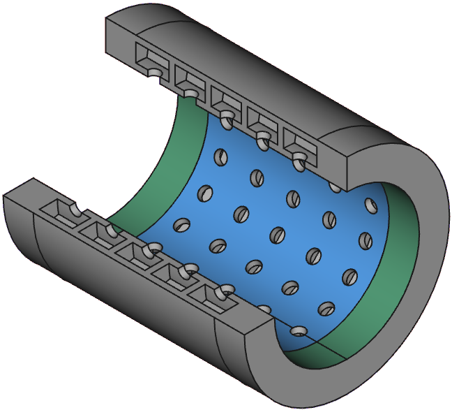
Refer to caption

Figure 3: A cylindrical liner for which in the limit δ→0\delta\to 0 the same impedance boundary conditions appear as for the considered flat surface.
Remark 2.6.

The following study is done on a flat interface Γ\Gamma for simplicity. For slow varying interfaces, the upcoming limit model can be derived using an appropriate variable change that flattens the surface. For the example of a cylindrical array of Helmholtz resonators, as it can be seen on Fig. 3, such a variable change has been used in a previous work[46].

3 Proof of the weak convergence to the limit

In this section, we derive the limit problem (2.11) on Ω\Omega using the two-scale convergence. To do so, we show that, up to a subsequence, (𝐯δ,pδ)({\mathbf{v}}^{\delta},p^{\delta}) converges weakly in H⁡(div,Ω)×H1​(Ω)\mathrm{H}(\Div,\Omega)\times\mathrm{H}^{1}(\Omega) to a limit (𝐯0,p0)({\mathbf{v}}_{0},p_{0}) that satisfies an Helmholtz-∇div\nabla\Div equation with radiation conditions. To obtain this result we prove the weak convergence of 𝐯δ{\mathbf{v}}^{\delta} in each subpart of Ωδ\Omega^{\delta}, i. e., the domain Ω\Omega not including the interface Γ\Gamma, the array of resonator chambers, the two-semi infinites strips of the pattern ℬδ\mathcal{B}^{\delta} and the array of resonator apertures, where matching conditions and finally impedance conditions follow.

From this stability result, we defive another a priori error estimate on what we will call the extended Helmholtz resonator array. We first extend the Helmholtz resonator ΩHδ​(𝐱Γδ)\Omega^{\delta}_{H}({\mathbf{x}}^{\delta}_{\Gamma}) centered at 𝐱Γδ{\mathbf{x}}^{\delta}_{\Gamma} into an extended Helmholtz resonator Ω~Hδ​(𝐱Γδ)\tilde{\Omega}^{\delta}_{H}({\mathbf{x}}^{\delta}_{\Gamma}) defined as

Ω~Hδ​(𝐱Γδ)=ΩHδ​(𝐱Γδ)∪(𝐱Γδ+𝒜×(0,2​δ)).\tilde{\Omega}^{\delta}_{H}({\mathbf{x}}^{\delta}_{\Gamma})=\Omega^{\delta}_{H}({\mathbf{x}}^{\delta}_{\Gamma})\cup\big({\mathbf{x}}^{\delta}_{\Gamma}+\mathcal{A}\times(0,2\sqrt{\delta})\big).
Lemma 3.1.

Let ω∉Λ\omega\not\in\Lambda, and let the assumption estimate (2.15) holds. There exists two constants CH>0C_{H}>0 and δ0>0\delta_{0}>0 such that, for any δ∈(0,δ0)\delta\in(0,\delta_{0}), the estimate

∑𝐱Γδ∈Γδ‖𝐯δ‖H⁡(div,Ω~Hδ​(𝐱Γδ))2+∑𝐱Γδ∈Γδδ2​‖𝐜𝐮𝐫𝐥⁡𝐯δ‖L2​(Ω~Hδ​(𝐱Γδ))32+∑𝐱Γδ∈Γδ‖pδ‖H1​(Ω~Hδ​(𝐱Γδ))2⩽CH.\sum_{{\mathbf{x}}^{\delta}_{\Gamma}\in\Gamma^{\delta}}\left\lVert{\mathbf{v}}^{\delta}\right\rVert_{\mathrm{H}(\Div,\tilde{\Omega}^{\delta}_{H}({\mathbf{x}}^{\delta}_{\Gamma}))}^{2}+\sum_{{\mathbf{x}}^{\delta}_{\Gamma}\in\Gamma^{\delta}}\delta^{2}\left\lVert\Curl{\mathbf{v}}^{\delta}\right\rVert_{\mathrm{L}^{2}(\tilde{\Omega}^{\delta}_{H}({\mathbf{x}}^{\delta}_{\Gamma}))^{3}}^{2}\\ +\sum_{{\mathbf{x}}^{\delta}_{\Gamma}\in\Gamma^{\delta}}\left\lVert p^{\delta}\right\rVert_{\mathrm{H}^{1}(\tilde{\Omega}^{\delta}_{H}({\mathbf{x}}^{\delta}_{\Gamma}))}^{2}\leqslant C_{H}. (3.1)

holds.

Proof.

Let ω∉Λ\omega\not\in\Lambda, and let the assumption estimate (2.15) holds. Taking the square of this estimate, and using that the union of all Ω~Hδ​(𝐱Γδ)\tilde{\Omega}^{\delta}_{H}({\mathbf{x}}^{\delta}_{\Gamma}) over 𝐱Γδ{\mathbf{x}}^{\delta}_{\Gamma} is a subset of Ωδ\Omega^{\delta} leads to estimate (3.1) with CH=3​CΩ2C_{H}=3C_{\Omega}^{2}. ∎

In the following, we use the estimate of this Lemma in each subsection: the array of Helmholtz resonators, the array of patterns below apertures, the array of apertures and the array of patterns above apertures.

3.1 Weak convergence in the resonator array

In this section, we consider for each δ>0\delta>0, 𝐱=(x1,x2,x3)∈Ωδ{\mathbf{x}}=(x_{1},x_{2},x_{3})\in\Omega^{\delta} with x3<−δx_{3}<-\sqrt{\delta}. At the first glance, we have to study positions 𝐱{\mathbf{x}} depending on δ\delta, since the location of each Helmholtz resonator depends on δ\delta. However, later we will see how to separate these dependencies.

Due to the geometrical assumption on the array of Helmholtz resonators, for each 𝐱{\mathbf{x}} in the array of Helmholtz resonators, there exists a center of aperture of one resonator, which we call resonator position 𝐱Γδ∈Γδ{\mathbf{x}}^{\delta}_{\Gamma}\in\Gamma^{\delta} such that 𝐱∈ΩCδ​(𝐱Γδ){\mathbf{x}}\in\Omega^{\delta}_{C}({\mathbf{x}}^{\delta}_{\Gamma}). We introduce the two-dimensional point 𝐲∈𝒜C{\mathbf{y}}\in\mathcal{A}_{C}, that we identify with abuse of notation to the three-dimensional point (𝐲,0)({\mathbf{y}},0), such that

𝐱↦(𝐲,x3):=(1δ​(𝐱−𝐱Γδ),x3)∈𝒜C×(−L,−δ),{\mathbf{x}}\mapsto({\mathbf{y}},x_{3}):=\big(\tfrac{1}{\delta}\big({\mathbf{x}}-{\mathbf{x}}^{\delta}_{\Gamma}\big),x_{3}\big)\in\mathcal{A}_{C}\times(-L,-\sqrt{\delta}),

i. e., 𝐱=𝐱Γδ+(0,0,x3)+δ​𝐲{\mathbf{x}}={\mathbf{x}}^{\delta}_{\Gamma}+(0,0,x_{3})+\delta{\mathbf{y}}. Using the coordinate (𝐲,x3)({\mathbf{y}},x_{3}) means to stretch the resonator ΩHδ​(𝐱Γδ)\Omega^{\delta}_{H}({\mathbf{x}}^{\delta}_{\Gamma})in the transverse plane (𝐞1,𝐞2)({\mathbf{e}}_{1},{\mathbf{e}}_{2}), and in this plane only. The stretched resonator chamber is denoted by Ω^Cδ:=𝒜C×(−L,−δ)\widehat{\Omega}^{\delta}_{C}:=\mathcal{A}_{C}\times(-L,-\sqrt{\delta}).

In the following, we introduce the five-dimensional functions 𝐕δ{\mathbf{V}}^{\delta} and PδP^{\delta}, depending on the resonator position 𝐱Γδ{\mathbf{x}}^{\delta}_{\Gamma}, the slow longitudinal variable x3x_{3} and the fast transverse variable 𝐲{\mathbf{y}}, by

𝐕δ​(𝐱Γδ,x3,𝐲)\displaystyle{\mathbf{V}}^{\delta}({\mathbf{x}}^{\delta}_{\Gamma},x_{3},{\mathbf{y}}) =𝐯δ​(𝐱Γδ+(0,0,x3)+δ​𝐲),\displaystyle={\mathbf{v}}^{\delta}({\mathbf{x}}^{\delta}_{\Gamma}+(0,0,x_{3})+\delta{\mathbf{y}}), (3.2)
Pδ​(𝐱Γδ,x3,𝐲)\displaystyle P^{\delta}({\mathbf{x}}^{\delta}_{\Gamma},x_{3},{\mathbf{y}}) =pδ​(𝐱Γδ+(0,0,x3)+δ​𝐲).\displaystyle=p^{\delta}({\mathbf{x}}^{\delta}_{\Gamma}+(0,0,x_{3})+\delta{\mathbf{y}}).

Considering the linearized Navier-Stokes problem (2.5) with the Laplace operator written as Δ=∇div−𝐜𝐮𝐫𝐥𝐜𝐮𝐫𝐥\Delta=\nabla\Div-\Curl\Curl and applying the anisotropic coordinate change, we obtain the system

−i​ω​𝐕δ+1δ​ρ0​∇𝐲Pδ+1ρ0​∂x3Pδ​𝐞3\displaystyle-\mathrm{i}\omega{\mathbf{V}}^{\delta}+\tfrac{1}{\delta\rho_{0}}\nabla_{{\mathbf{y}}}P^{\delta}+\tfrac{1}{\rho_{0}}\partial_{x_{3}}P^{\delta}{\mathbf{e}}_{3} (3.3a)
−(ν0+ν0′)​δ2​∇𝐲div𝐲​𝐕δ\displaystyle-(\nu_{0}+\nu_{0}^{\prime})\delta^{2}\nabla_{{\mathbf{y}}}\Div_{\mathbf{y}}{\mathbf{V}}^{\delta}
−(ν0+ν0′)δ2∂𝐞3div𝐲𝐕δ𝐞3−\displaystyle-(\nu_{0}+\nu_{0}^{\prime})\delta^{2}\partial_{{\mathbf{e}}_{3}}\Div_{\mathbf{y}}{\mathbf{V}}^{\delta}{\mathbf{e}}_{3}-
(ν0+ν0′)​δ3​∇𝐲(∂x3𝐕δ⋅𝐞3)\displaystyle(\nu_{0}+\nu_{0}^{\prime})\delta^{3}\nabla_{{\mathbf{y}}}\big(\partial_{x_{3}}{\mathbf{V}}^{\delta}\cdot{\mathbf{e}}_{3}\big)
−(ν0+ν0′)δ4∂x3(∂x3𝐕δ⋅𝐞3)\displaystyle-(\nu_{0}+\nu_{0}^{\prime})\delta^{4}\partial_{x_{3}}\big(\partial_{x_{3}}{\mathbf{V}}^{\delta}\cdot{\mathbf{e}}_{3}\big)
+ν0δ4(1δ∂y1,1δ∂y2,∂x3)∧((1δ∂y1,1δ∂y2,∂x3)∧𝐕δ)\displaystyle+\nu_{0}\delta^{4}\big(\tfrac{1}{\delta}\partial_{y_{1}},\tfrac{1}{\delta}\partial_{y_{2}},\partial_{x_{3}}\big)\wedge\Big(\big(\tfrac{1}{\delta}\partial_{y_{1}},\tfrac{1}{\delta}\partial_{y_{2}},\partial_{x_{3}}\big)\wedge{\mathbf{V}}^{\delta}\Big) =𝟎,in ​Γδ×Ω^Cδ,\displaystyle=\bm{0},\quad\text{in }\Gamma^{\delta}\times\widehat{\Omega}^{\delta}_{C},
−i​ω​Pδ+ρ0​c2δ​div𝐲​𝐕δ+ρ0​c2​(∂x3𝐕δ⋅𝐞3)\displaystyle-\mathrm{i}\omega P^{\delta}+\tfrac{\rho_{0}c^{2}}{\delta}\Div_{{\mathbf{y}}}{\mathbf{V}}^{\delta}+\rho_{0}c^{2}\big(\partial_{x_{3}}{\mathbf{V}}^{\delta}\cdot{\mathbf{e}}_{3}\big) =0,in Γδ×Ω^δC,\displaystyle=0,\quad\text{in }\Gamma^{\delta}\times\widehat{\Omega}^{\delta}_{C}, (3.3b)
𝐕δ\displaystyle{\mathbf{V}}^{\delta} =𝟎,on ​Γδ×(−L,−δ)×∂𝒜C,\displaystyle=\bm{0},\quad\text{on }\Gamma^{\delta}\times(-L,-\sqrt{\delta})\times\partial\mathcal{A}_{C}, (3.3c)
𝐕δ\displaystyle{\mathbf{V}}^{\delta} =𝟎,on ​Γδ×{−L}×𝒜C.\displaystyle=\bm{0},\quad\text{on }\Gamma^{\delta}\times\{-L\}\times\mathcal{A}_{C}. (3.3d)

The estimate (3.1) of the Lemma 3.1 is equivalent to state in rescaled coordinates that

∑𝐱Γδ∈Γδ‖𝐕δ​(𝐱Γδ,⋅)‖L2​(Ω^Cδ)32+1δ2​∑𝐱Γδ∈Γδ‖div𝐲⁡𝐕δ‖L2​(Ω^Cδ)2+∑𝐱Γδ∈Γδ‖∂x3𝐕δ(𝐱Γδ,⋅)⋅𝐞3‖L2​(Ω^Cδ)2+δ4∑𝐱Γδ∈Γδ‖(1δ∂y1,1δ∂y2,∂x3)∧𝐕δ(𝐱δΓ,⋅)‖L2​(Ω^Cδ)32+∑𝐱Γδ∈Γδ‖Pδ(𝐱δΓ,⋅)‖L2​(Ω^Cδ)2+1δ2∑𝐱Γδ∈Γδ‖∇𝐲pδ(𝐱δΓ,⋅)‖L2​(Ω~Hδ​(𝐱Γδ))22+∑𝐱Γδ∈Γδ‖∂x3Pδ(𝐱δΓ,⋅)‖L2​(Ω^Cδ)2⩽CH.\sum_{{\mathbf{x}}^{\delta}_{\Gamma}\in\Gamma^{\delta}}\left\lVert{\mathbf{V}}^{\delta}({\mathbf{x}}_{\Gamma}^{\delta},\cdot)\right\rVert_{\mathrm{L}^{2}(\widehat{\Omega}^{\delta}_{C})^{3}}^{2}+\tfrac{1}{\delta^{2}}\sum_{{\mathbf{x}}^{\delta}_{\Gamma}\in\Gamma^{\delta}}\left\lVert\Div_{\mathbf{y}}{\mathbf{V}}^{\delta}\right\rVert_{\mathrm{L}^{2}(\widehat{\Omega}^{\delta}_{C})}^{2}\\ +\sum_{{\mathbf{x}}^{\delta}_{\Gamma}\in\Gamma^{\delta}}\left\lVert\partial_{x_{3}}{\mathbf{V}}^{\delta}({\mathbf{x}}_{\Gamma}^{\delta},\cdot)\cdot{\mathbf{e}}_{3}\right\rVert_{\mathrm{L}^{2}(\widehat{\Omega}^{\delta}_{C})}^{2}+\delta^{4}\sum_{{\mathbf{x}}^{\delta}_{\Gamma}\in\Gamma^{\delta}}\left\lVert\big(\tfrac{1}{\delta}\partial_{y_{1}},\tfrac{1}{\delta}\partial_{y_{2}},\partial_{x_{3}}\big)\wedge{\mathbf{V}}^{\delta}({\mathbf{x}}^{\delta}_{\Gamma},\cdot)\right\rVert_{\mathrm{L}^{2}(\widehat{\Omega}^{\delta}_{C})^{3}}^{2}\\ +\sum_{{\mathbf{x}}^{\delta}_{\Gamma}\in\Gamma^{\delta}}\left\lVert P^{\delta}({\mathbf{x}}^{\delta}_{\Gamma},\cdot)\right\rVert_{\mathrm{L}^{2}(\widehat{\Omega}^{\delta}_{C})}^{2}+\tfrac{1}{\delta^{2}}\sum_{{\mathbf{x}}^{\delta}_{\Gamma}\in\Gamma^{\delta}}\left\lVert\nabla_{\mathbf{y}}p^{\delta}({\mathbf{x}}^{\delta}_{\Gamma},\cdot)\right\rVert_{\mathrm{L}^{2}(\tilde{\Omega}^{\delta}_{H}({\mathbf{x}}^{\delta}_{\Gamma}))^{2}}^{2}\\ +\sum_{{\mathbf{x}}^{\delta}_{\Gamma}\in\Gamma^{\delta}}\left\lVert\partial_{x_{3}}P^{\delta}({\mathbf{x}}^{\delta}_{\Gamma},\cdot)\right\rVert_{\mathrm{L}^{2}(\widehat{\Omega}^{\delta}_{C})}^{2}\leqslant C_{H}. (3.4)

The main idea is to extend the functions (𝐕δ,Pδ)({\mathbf{V}}^{\delta},P^{\delta}) discrete with respect to 𝐱Γδ∈Γδ{\mathbf{x}}^{\delta}_{\Gamma}\in\Gamma^{\delta} to functions still denoted by (𝐕δ,Pδ)({\mathbf{V}}^{\delta},P^{\delta}) and continuous with respect to 𝐱∈Γ{\mathbf{x}}\in\Gamma by the following

(𝐕δ,Pδ)​(𝐱Γ,⋅)=(𝐕δ,Pδ)​(𝐱Γδ,⋅),𝐱Γ∈𝐱Γδ+δ​𝒜.({\mathbf{V}}^{\delta},P^{\delta})({\mathbf{x}}_{\Gamma},\cdot)=({\mathbf{V}}^{\delta},P^{\delta})({\mathbf{x}}^{\delta}_{\Gamma},\cdot),\quad{\mathbf{x}}_{\Gamma}\in{\mathbf{x}}^{\delta}_{\Gamma}+\delta\mathcal{A}.

The equation (3.3) is then extended naturally on 𝐱Γ∈Γ{\mathbf{x}}_{\Gamma}\in\Gamma (the parameter 𝐱Γδ{\mathbf{x}}^{\delta}_{\Gamma} is only playing a parameter), and the discrete error estimate (3.4) is extended to a continuous error estimate

‖𝐕δ‖L2​(Γ,L2​(Ω^Cδ)3)2+1δ2​‖div𝐲⁡𝐕δ‖L2​(Γ,L2​(Ω^Cδ))2+‖∂x3𝐕δ⋅𝐞3‖L2​(Γ,L2​(Ω^Cδ))2+δ4‖(1δ∂y1,1δ∂y2,∂x3)∧𝐕δ‖L2​(Γ,L2​(Ω^Cδ)3)2+‖Pδ‖L2​(Γ,L2​(Ω^Cδ))2+1δ2​‖∇𝐲Pδ‖L2​(Γ,L2​(Ω^Cδ)2)2+‖∂x3Pδ‖L2​(Γ,L2​(Ω^Cδ))2⩽CH​|𝒜|.\left\lVert{\mathbf{V}}^{\delta}\right\rVert_{\mathrm{L}^{2}(\Gamma;\mathrm{L}^{2}(\widehat{\Omega}^{\delta}_{C})^{3})}^{2}+\tfrac{1}{\delta^{2}}\left\lVert\Div_{{\mathbf{y}}}{\mathbf{V}}^{\delta}\right\rVert_{\mathrm{L}^{2}(\Gamma;\mathrm{L}^{2}(\widehat{\Omega}^{\delta}_{C}))}^{2}+\left\lVert\partial_{x_{3}}{\mathbf{V}}^{\delta}\cdot{\mathbf{e}}_{3}\right\rVert_{\mathrm{L}^{2}(\Gamma;\mathrm{L}^{2}(\widehat{\Omega}^{\delta}_{C}))}^{2}\\ +\delta^{4}\left\lVert\big(\tfrac{1}{\delta}\partial_{y_{1}},\tfrac{1}{\delta}\partial_{y_{2}},\partial_{x_{3}}\big)\wedge{\mathbf{V}}^{\delta}\right\rVert_{\mathrm{L}^{2}(\Gamma;\mathrm{L}^{2}(\widehat{\Omega}^{\delta}_{C})^{3})}^{2}+\left\lVert P^{\delta}\right\rVert_{\mathrm{L}^{2}(\Gamma;\mathrm{L}^{2}(\widehat{\Omega}^{\delta}_{C}))}^{2}\\ +\frac{1}{\delta^{2}}\left\lVert\nabla_{\mathbf{y}}P^{\delta}\right\rVert_{\mathrm{L}^{2}(\Gamma;\mathrm{L}^{2}(\widehat{\Omega}^{\delta}_{C})^{2})}^{2}+\left\lVert\partial_{x_{3}}P^{\delta}\right\rVert_{\mathrm{L}^{2}(\Gamma;\mathrm{L}^{2}(\widehat{\Omega}^{\delta}_{C}))}^{2}\leqslant C_{H}|\mathcal{A}|. (3.5)

This means that the sequence (𝐕δ,Pδ)({\mathbf{V}}^{\delta},P^{\delta}) is bounded in L2​(Γ,H⁡(div,Ω^Cδ))×L2​(Γ,H1​(Ω^Cδ))\mathrm{L}^{2}(\Gamma;\mathrm{H}(\Div,\widehat{\Omega}^{\delta}_{C}))\times\mathrm{L}^{2}(\Gamma;\mathrm{H}^{1}(\widehat{\Omega}^{\delta}_{C})), independent of δ→0\delta\to 0 even the domain Ω^Cδ\widehat{\Omega}^{\delta}_{C} enlarges for decreasing δ\delta. Then, for any fixed ε>0\varepsilon>0 and for any δ<ε\delta<\varepsilon, the sequence (𝐕δ,Pδ)({\mathbf{V}}^{\delta},P^{\delta}) is bounded in L2​(Γ,H⁡(div,Ω^Cε))×L2​(Γ,H1​(Ω^Cε))\mathrm{L}^{2}(\Gamma;\mathrm{H}(\Div,\widehat{\Omega}^{\varepsilon}_{C}))\times\mathrm{L}^{2}(\Gamma;\mathrm{H}^{1}(\widehat{\Omega}^{\varepsilon}_{C})) therefore we can extract a subsequence that we still denote by (𝐕δ,Pδ)({\mathbf{V}}^{\delta},P^{\delta}) that converges to a limit (𝐕0ε,P0ε)({\mathbf{V}}_{0}^{\varepsilon},P_{0}^{\varepsilon}) weakly in L2​(Γ,H⁡(div,Ω^Cε))×L2​(Γ,H1​(Ω^Cε))\mathrm{L}^{2}(\Gamma;\mathrm{H}(\Div,\widehat{\Omega}^{\varepsilon}_{C}))\times\mathrm{L}^{2}(\Gamma;\mathrm{H}^{1}(\widehat{\Omega}^{\varepsilon}_{C})). Combining the lower semi-continuity of the weak limit stated by the Theorem 2.2.1 of the book of Evans[16] with the estimate (3.5), we find

‖∇𝐲P0ε‖L2​(Γ,L2​(Ω^Cε)2)⩽lim infδ→0‖∇𝐲Pδ‖L2​(Γ,L2​(Ω^Cδ)2)⩽lim infδ→0δ​CH​|𝒜|=0.\left\lVert\nabla_{\mathbf{y}}P_{0}^{\varepsilon}\right\rVert_{\mathrm{L}^{2}(\Gamma;\mathrm{L}^{2}(\widehat{\Omega}^{\varepsilon}_{C})^{2})}\leqslant\liminf_{\delta\to 0}\left\lVert\nabla_{\mathbf{y}}P^{\delta}\right\rVert_{\mathrm{L}^{2}(\Gamma;\mathrm{L}^{2}(\widehat{\Omega}^{\delta}_{C})^{2})}\leqslant\liminf_{\delta\to 0}\delta\sqrt{C_{H}|\mathcal{A}|}=0.

This motivates us to take the scalar product of (3.3) with test functions (𝐖,Q)({\mathbf{W}},Q) with QQ independent of the fast transverse variable 𝐲{\mathbf{y}}. Then, integrating by parts equation (3.3) leads to

−i​ω​⟨𝐕δ​(𝐱Γ,⋅),𝐖⟩(Ω^Cε)3+1ρ0​⟨∂x3Pδ​(𝐱Γ,⋅)​𝐞3,𝐖⟩(Ω^Cε)3\displaystyle-\mathrm{i}\omega\left<{\mathbf{V}}^{\delta}({\mathbf{x}}_{\Gamma},\cdot),{\mathbf{W}}\right>_{(\widehat{\Omega}^{\varepsilon}_{C})^{3}}+\tfrac{1}{\rho_{0}}\left<\partial_{x_{3}}P^{\delta}({\mathbf{x}}_{\Gamma},\cdot){\mathbf{e}}_{3},{\mathbf{W}}\right>_{(\widehat{\Omega}^{\varepsilon}_{C})^{3}} (3.6)
−ν0δ4⟨(1δ∂y1,1δ∂y2,∂x3)∧𝐕δ(𝐱Γ,⋅),(0,0,∂x3)∧𝐖⟩(Ω^Cε)3\displaystyle-\nu_{0}\delta^{4}\left<\big(\tfrac{1}{\delta}\partial_{y_{1}},\tfrac{1}{\delta}\partial_{y_{2}},\partial_{x_{3}}\big)\wedge{\mathbf{V}}^{\delta}({\mathbf{x}}_{\Gamma},\cdot),(0,0,\partial_{x_{3}})\wedge{\mathbf{W}}\right>_{(\widehat{\Omega}^{\varepsilon}_{C})^{3}}
+(ν0+ν0′)​δ2​⟨div𝐲⁡(𝐱Γ,⋅)​𝐕δ,div𝐲⁡𝐖⋅𝐞3⟩Ω^Cε\displaystyle+(\nu_{0}+\nu^{\prime}_{0})\delta^{2}\left<\Div_{\mathbf{y}}({\mathbf{x}}_{\Gamma},\cdot){\mathbf{V}}^{\delta},\Div_{\mathbf{y}}{\mathbf{W}}\cdot{\mathbf{e}}_{3}\right>_{\widehat{\Omega}^{\varepsilon}_{C}}
+(ν0+ν0′)​δ3​⟨∂x3(𝐱Γ,⋅)​𝐕δ,div𝐲⁡𝐖⋅𝐞3⟩Ω^Cε\displaystyle+(\nu_{0}+\nu^{\prime}_{0})\delta^{3}\left<\partial_{x_{3}}({\mathbf{x}}_{\Gamma},\cdot){\mathbf{V}}^{\delta},\Div_{\mathbf{y}}{\mathbf{W}}\cdot{\mathbf{e}}_{3}\right>_{\widehat{\Omega}^{\varepsilon}_{C}}
+(ν0+ν0′)​δ3​⟨div𝐲⁡(𝐱Γ,⋅)​𝐕δ,∂x3𝐖⋅𝐞3⟩Ω^Cε\displaystyle+(\nu_{0}+\nu^{\prime}_{0})\delta^{3}\left<\Div_{\mathbf{y}}({\mathbf{x}}_{\Gamma},\cdot){\mathbf{V}}^{\delta},\partial_{x_{3}}{\mathbf{W}}\cdot{\mathbf{e}}_{3}\right>_{\widehat{\Omega}^{\varepsilon}_{C}}
+(ν0+ν0′)​δ4​⟨∂x3𝐕δ​(𝐱Γ,⋅)⋅𝐞3,∂x3𝐖⋅𝐞3⟩Ω^Cε\displaystyle+(\nu_{0}+\nu^{\prime}_{0})\delta^{4}\left<\partial_{x_{3}}{\mathbf{V}}^{\delta}({\mathbf{x}}_{\Gamma},\cdot)\cdot{\mathbf{e}}_{3},\partial_{x_{3}}{\mathbf{W}}\cdot{\mathbf{e}}_{3}\right>_{\widehat{\Omega}^{\varepsilon}_{C}} =0,\displaystyle=0,
−i​ω​⟨Pδ​(𝐱Γ,⋅),Q⟩Ω^Cε+ρ0​c2​⟨∇𝐲𝐕δ​(𝐱Γ,⋅),Q⟩Ω^Cε\displaystyle-\mathrm{i}\omega\left<P^{\delta}({\mathbf{x}}_{\Gamma},\cdot),Q\right>_{\widehat{\Omega}^{\varepsilon}_{C}}+\rho_{0}c^{2}\left<\nabla_{\mathbf{y}}{\mathbf{V}}^{\delta}({\mathbf{x}}_{\Gamma},\cdot),Q\right>_{\widehat{\Omega}^{\varepsilon}_{C}}
+ρ0​c2​⟨∂x3𝐕δ​(𝐱Γ,⋅)⋅𝐞3,Q⟩Ω^Cε\displaystyle+\rho_{0}c^{2}\left<\partial_{x_{3}}{\mathbf{V}}^{\delta}({\mathbf{x}}_{\Gamma},\cdot)\cdot{\mathbf{e}}_{3},Q\right>_{\widehat{\Omega}^{\varepsilon}_{C}} =0.\displaystyle=0.

Then, using the weak convergence of (𝐕δ,Pδ)({\mathbf{V}}^{\delta},P^{\delta}) to (𝐕0ε,P0ε)({\mathbf{V}}_{0}^{\varepsilon},P_{0}^{\varepsilon}) in L2​(Γ,H⁡(div,Ω^Cε))×L2​(Γ,H1​(Ω^Cε))\mathrm{L}^{2}(\Gamma;\mathrm{H}(\Div,\widehat{\Omega}^{\varepsilon}_{C}))\times\mathrm{L}^{2}(\Gamma;\mathrm{H}^{1}(\widehat{\Omega}^{\varepsilon}_{C})) using estimate (3.5), we find the limit δ→0\delta\to 0 for almost all 𝐱Γ∈Γ{\mathbf{x}}_{\Gamma}\in\Gamma

−i​ω​⟨𝐕0ε​(𝐱Γ,⋅),𝐖⟩(Ω^Cε)3+1ρ0​⟨∂x3P0ε​(𝐱Γ,⋅)​𝐞3,𝐖⟩(Ω^Cε)3\displaystyle-\mathrm{i}\omega\left<{\mathbf{V}}_{0}^{\varepsilon}({\mathbf{x}}_{\Gamma},\cdot),{\mathbf{W}}\right>_{(\widehat{\Omega}^{\varepsilon}_{C})^{3}}+\tfrac{1}{\rho_{0}}\left<\partial_{x_{3}}P_{0}^{\varepsilon}({\mathbf{x}}_{\Gamma},\cdot){\mathbf{e}}_{3},{\mathbf{W}}\right>_{(\widehat{\Omega}^{\varepsilon}_{C})^{3}} =0,\displaystyle=0, (3.7a)
−i​ω​⟨P0ε​(𝐱Γ,⋅),Q⟩Ω^Cε+ρ0​c2​⟨∂x3𝐕0ε​(𝐱Γ,⋅)⋅𝐞3,Q⟩Ω^Cε\displaystyle-\mathrm{i}\omega\left<P_{0}^{\varepsilon}({\mathbf{x}}_{\Gamma},\cdot),Q\right>_{\widehat{\Omega}^{\varepsilon}_{C}}+\rho_{0}c^{2}\left<\partial_{x_{3}}{\mathbf{V}}_{0}^{\varepsilon}({\mathbf{x}}_{\Gamma},\cdot)\cdot{\mathbf{e}}_{3},Q\right>_{\widehat{\Omega}^{\varepsilon}_{C}} =0.\displaystyle=0. (3.7b)

The arbitrary choice of 𝐖{\mathbf{W}} leads to

−i​ω​𝐕0ε​(𝐱Γ,⋅)+1ρ0​∂x3P0ε​(𝐱Γ,⋅)​𝐞3=0,-\mathrm{i}\omega{\mathbf{V}}_{0}^{\varepsilon}({\mathbf{x}}_{\Gamma},\cdot)+\tfrac{1}{\rho_{0}}\partial_{x_{3}}P_{0}^{\varepsilon}({\mathbf{x}}_{\Gamma},\cdot){\mathbf{e}}_{3}=0,

and gives a posteriori that 𝐕0ε​(𝐱Γ,⋅){\mathbf{V}}_{0}^{\varepsilon}({\mathbf{x}}_{\Gamma},\cdot) is also independent of 𝐲{\mathbf{y}} and is directed among the 𝐞3{\mathbf{e}}_{3} direction, i. e., there exists a scalar function V0,3εV_{0,3}^{\varepsilon} independent of 𝐲{\mathbf{y}} such that

𝐕0ε​(𝐱Γ,x3,𝐲)=V0,3ε​(𝐱Γ,x3)​𝐞3.{\mathbf{V}}_{0}^{\varepsilon}({\mathbf{x}}_{\Gamma},x_{3},{\mathbf{y}})=V_{0,3}^{\varepsilon}({\mathbf{x}}_{\Gamma},x_{3}){\mathbf{e}}_{3}.

Taking then the equation (3.7b), we deduce that

−i​ω​P0ε​(𝐱Γ,⋅)+ρ0​c2​∂x3𝐕0ε​(𝐱Γ,⋅)⋅𝐞3=0,-\mathrm{i}\omega P_{0}^{\varepsilon}({\mathbf{x}}_{\Gamma},\cdot)+\rho_{0}c^{2}\partial_{x_{3}}{\mathbf{V}}_{0}^{\varepsilon}({\mathbf{x}}_{\Gamma},\cdot)\cdot{\mathbf{e}}_{3}=0,

i. e., that (𝐕0ε​(𝐱Γ,⋅),P0ε​(𝐱Γ,⋅))({\mathbf{V}}_{0}^{\varepsilon}({\mathbf{x}}_{\Gamma},\cdot),P_{0}^{\varepsilon}({\mathbf{x}}_{\Gamma},\cdot)) is solution of an homogeneous one-dimensional Helmholtz equation. Derivation of the boundary condition at x3=−Lx_{3}=-L is done as follow: we take a particular test function WW depending on (x3,𝐲)∈(−L,0)×𝒜C(x_{3},{\mathbf{y}})\in(-L,0)\times\mathcal{A}_{C} such that W⁡(x3,𝐲)=1W(x_{3},{\mathbf{y}})=1 for x3<−3L/4x_{3}<-3L/4 and W⁡(x3,𝐲)=0W(x_{3},{\mathbf{y}})=0 for x3>−L/2x_{3}>-L/2, and using a one-dimensional Stokes formula coupled to the weak convergence of 𝐕δ{\mathbf{V}}^{\delta} to V0,3ε​𝐞3V^{\varepsilon}_{0,3}{\mathbf{e}}_{3} in (L2​(Γ,L2​(Ω^Cδ))CLOSE(\mathrm{L}^{2}(\Gamma;\mathrm{L}^{2}(\widehat{\Omega}^{\delta}_{C})) gives

0=limδ→0∫𝒜C{∂x3(𝐕δ(𝐱Γ,x3,𝐲)⋅𝐞3−Vε0,3(𝐱Γ,x3))W(x3)+(𝐕δ(𝐱Γ,x3,𝐲)⋅𝐞3−Vε0,3(𝐱Γ,x3))∂x3W(x3)}d𝐲dx3=−aCVε0,3(𝐱Γ,x3),0=\lim_{\delta\to 0}\int_{\mathcal{A}_{C}}\Big\{\partial_{x_{3}}({\mathbf{V}}^{\delta}({\mathbf{x}}_{\Gamma},x_{3},{\mathbf{y}})\cdot{\mathbf{e}}_{3}-V^{\varepsilon}_{0,3}({\mathbf{x}}_{\Gamma},x_{3}))W(x_{3})\\ +({\mathbf{V}}^{\delta}({\mathbf{x}}_{\Gamma},x_{3},{\mathbf{y}})\cdot{\mathbf{e}}_{3}-V^{\varepsilon}_{0,3}({\mathbf{x}}_{\Gamma},x_{3}))\partial_{x_{3}}W(x_{3})\Big\}\,\mathrm{d}{\mathbf{y}}\,\mathrm{d}x_{3}=-a_{C}V^{\varepsilon}_{0,3}({\mathbf{x}}_{\Gamma},x_{3}),

so there exists a scalar function V0εV^{\varepsilon}_{0} depending only on the resonator position such that

𝐕0ε​(𝐱Γ,x3)\displaystyle{\mathbf{V}}^{\varepsilon}_{0}({\mathbf{x}}_{\Gamma},x_{3}) =V0ε​(𝐱Γ)​sin⁡(ωc​(L+x3))\displaystyle=V^{\varepsilon}_{0}({\mathbf{x}}_{\Gamma})\sin\big(\tfrac{\omega}{c}(L+x_{3})\big) (3.8)
P0ε​(𝐱Γ,x3)\displaystyle P^{\varepsilon}_{0}({\mathbf{x}}_{\Gamma},x_{3}) =−i​ρ0​c​V0ε​(𝐱Γ)​cos⁡(ωc​(L+x3)).\displaystyle=-\mathrm{i}\rho_{0}cV^{\varepsilon}_{0}({\mathbf{x}}_{\Gamma})\cos\big(\tfrac{\omega}{c}(L+x_{3})\big).

The next point is to derive a limit problem on the domain Ω^C:=limε→0Ω^Cε=𝒜C×(−L,0)\widehat{\Omega}_{C}:=\lim_{\varepsilon\to 0}\widehat{\Omega}_{C}^{\varepsilon}=\mathcal{A}_{C}\times(-L,0). To do so, using the lower semi-continuity of the weak limit (𝐕0ε,P0ε)({\mathbf{V}}_{0}^{\varepsilon},P^{\varepsilon}_{0}) with the a priori estimate (3.5), it holds

‖𝐕0ε‖L2​(Γ,L2​(Ω^Cε))2+‖∂x3𝐕0ε‖L2​(Γ,L2​(Ω^Cε))2+‖P0ε‖L2​(Γ,L2​(Ω^Cε))2+‖∂x3P0ε‖L2​(Γ,L2​(Ω^Cε))2⩽CH​|𝒜|.\left\lVert{\mathbf{V}}_{0}^{\varepsilon}\right\rVert_{\mathrm{L}^{2}(\Gamma,\mathrm{L}^{2}(\widehat{\Omega}^{\varepsilon}_{C}))}^{2}+\left\lVert\partial_{x_{3}}{\mathbf{V}}_{0}^{\varepsilon}\right\rVert_{\mathrm{L}^{2}(\Gamma,\mathrm{L}^{2}(\widehat{\Omega}^{\varepsilon}_{C}))}^{2}\\ +\left\lVert P_{0}^{\varepsilon}\right\rVert_{\mathrm{L}^{2}(\Gamma,\mathrm{L}^{2}(\widehat{\Omega}^{\varepsilon}_{C}))}^{2}+\left\lVert\partial_{x_{3}}P_{0}^{\varepsilon}\right\rVert_{\mathrm{L}^{2}(\Gamma,\mathrm{L}^{2}(\widehat{\Omega}^{\varepsilon}_{C}))}^{2}\leqslant C_{H}|\mathcal{A}|.

This error estimate combined to (3.8) leads to

(1+ω2c2+ρ02​c2+ρ02​ω2)​(L−ε)​‖V0ε‖L2​(Γ)2⩽2​CH​|𝒜|.\big(1+\tfrac{\omega^{2}}{c^{2}}+\rho_{0}^{2}c^{2}+\rho_{0}^{2}\omega^{2}\big)(L-\sqrt{\varepsilon})\left\lVert V^{\varepsilon}_{0}\right\rVert_{\mathrm{L}^{2}(\Gamma)}^{2}\leqslant 2C_{H}|\mathcal{A}|.

Extending (𝐕0ε,P0ε)({\mathbf{V}}^{\varepsilon}_{0},P^{\varepsilon}_{0}) on 𝒜×(−L,0)\mathcal{A}\times(-L,0) using formula (3.8) and using this last error estimate leads to, for 2​ε<L2\sqrt{\varepsilon}<L,

‖𝐕0ε‖L2​(Γ,L2​(Ω^C0))2+‖∂x3𝐕0ε‖L2​(Γ,L2​(Ω^C0))2+‖P0ε‖L2​(Γ,L2​(Ω^C0))2+‖∂x3P0ε‖L2​(Γ,L2​(Ω^C0))2⩽2​L(L−ε)​CH​|𝒜|⩽4​CH​|𝒜|.\left\lVert{\mathbf{V}}_{0}^{\varepsilon}\right\rVert_{\mathrm{L}^{2}(\Gamma,\mathrm{L}^{2}(\widehat{\Omega}^{0}_{C}))}^{2}+\left\lVert\partial_{x_{3}}{\mathbf{V}}_{0}^{\varepsilon}\right\rVert_{\mathrm{L}^{2}(\Gamma,\mathrm{L}^{2}(\widehat{\Omega}^{0}_{C}))}^{2}\\ +\left\lVert P_{0}^{\varepsilon}\right\rVert_{\mathrm{L}^{2}(\Gamma,\mathrm{L}^{2}(\widehat{\Omega}^{0}_{C}))}^{2}+\left\lVert\partial_{x_{3}}P_{0}^{\varepsilon}\right\rVert_{\mathrm{L}^{2}(\Gamma,\mathrm{L}^{2}(\widehat{\Omega}^{0}_{C}))}^{2}\leqslant\tfrac{2L}{(L-\sqrt{\varepsilon})}C_{H}|\mathcal{A}|\leqslant 4C_{H}|\mathcal{A}|.

so that (𝐕0ε,P0ε)({\mathbf{V}}^{\varepsilon}_{0},P^{\varepsilon}_{0}) is uniformly bounded in L2​(Γ,H⁡(div,Ω^C)×H1​(Ω^C))\mathrm{L}^{2}(\Gamma;\mathrm{H}(\Div;\widehat{\Omega}_{C})\times\mathrm{H}^{1}(\widehat{\Omega}_{C})). There exists then a subsequence that we still denote by (𝐕0ε,P0ε)({\mathbf{V}}^{\varepsilon}_{0},P^{\varepsilon}_{0}) that weakly converges to a limit (𝐕0,P0)∈L2​(Γ,H⁡(div,Ω^C)×H1​(Ω^C))({\mathbf{V}}_{0},P_{0})\in\mathrm{L}^{2}(\Gamma;\mathrm{H}(\Div;\widehat{\Omega}_{C})\times\mathrm{H}^{1}(\widehat{\Omega}_{C})).

We have two small quantities, δ\delta and ε\varepsilon, and we want to make these two quantities tending to 00. To do so, we will make a diagonal construction of (𝐕δ,Pδ)({\mathbf{V}}^{\delta},P^{\delta}) to (V0,3​𝐞3,P0)(V_{0,3}{\mathbf{e}}_{3},P_{0}) by the following

  1. 1.

    (𝐕δ,Pδ)({\mathbf{V}}^{\delta},P^{\delta}) is bounded in L2​(Γ,(H⁡(div,Ω^Cε1))3×H1​(Ω^Cε1))\mathrm{L}^{2}\big(\Gamma;(\mathrm{H}(\Div;\widehat{\Omega}^{\varepsilon_{1}}_{C}))^{3}\times\mathrm{H}^{1}(\widehat{\Omega}^{\varepsilon_{1}}_{C})\big) using the energy estimate (3.5) for any δ⩽ε1\delta\leqslant\varepsilon_{1}, so there exists a sequence (𝐕δn(1),Pδn(1))n∈ℕ({\mathbf{V}}^{\delta_{n}^{(1)}},P^{\delta_{n}^{(1)}})_{n\in{\mathbb{N}}} that weakly converges to (𝐕ε1,Pε1)({\mathbf{V}}^{\varepsilon_{1}},P^{\varepsilon_{1}}) L2​(Γ,(H⁡(div,Ω^Cε1))×H1​(Ω^Cε1))\mathrm{L}^{2}\big(\Gamma;(\mathrm{H}(\Div;\widehat{\Omega}^{\varepsilon_{1}}_{C}))\times\mathrm{H}^{1}(\widehat{\Omega}^{\varepsilon_{1}}_{C})\big). We consider the sequence of decreasing indices (δn(1))n∈ℕ(\delta_{n}^{(1)})_{n\in{\mathbb{N}}} such that δ0(1)⩽ε2\delta_{0}^{(1)}\leqslant\varepsilon_{2},

  2. 2.

    (𝐕δn(1),Pδn(1))n∈ℕ({\mathbf{V}}^{\delta_{n}^{(1)}},P^{\delta_{n}^{(1)}})_{n\in{\mathbb{N}}} is bounded in L2​(Γ,(H⁡(div,Ω^Cε2))×H1​(Ω^Cε2))\mathrm{L}^{2}\big(\Gamma;(\mathrm{H}(\Div;\widehat{\Omega}^{\varepsilon_{2}}_{C}))\times\mathrm{H}^{1}(\widehat{\Omega}^{\varepsilon_{2}}_{C})\big) using the energy estimate (3.5) since δn(1)⩽δ0(1)⩽ε2\delta_{n}^{(1)}\leqslant\delta_{0}^{(1)}\leqslant\varepsilon_{2} for any n∈ℕn\in{\mathbb{N}}, so there exists a subsequence (𝐕δn(2),Pδn(2))({\mathbf{V}}^{\delta_{n}^{(2)}},P^{\delta_{n}^{(2)}}) that weakly converges to (𝐕ε2,Pε2)({\mathbf{V}}^{\varepsilon_{2}},P^{\varepsilon_{2}}) L2​(Γ,(H⁡(div,Ω^Cε2))×H1​(Ω^Cε2))\mathrm{L}^{2}\big(\Gamma;(\mathrm{H}(\Div;\widehat{\Omega}^{\varepsilon_{2}}_{C}))\times\mathrm{H}^{1}(\widehat{\Omega}^{\varepsilon_{2}}_{C})\big). We consider the sequence of decreasing indices (δn(2))n∈ℕ(\delta_{n}^{(2)})_{n\in{\mathbb{N}}} such that δ0(2)⩽ε3\delta_{0}^{(2)}\leqslant\varepsilon_{3}. Finally due to the extraction process, it holds that (𝐕ε2,Pε2)=(𝐕ε1,Pε1)({\mathbf{V}}^{\varepsilon_{2}},P^{\varepsilon_{2}})=({\mathbf{V}}^{\varepsilon_{1}},P^{\varepsilon_{1}}) on Ω^Cε1\widehat{\Omega}^{\varepsilon_{1}}_{C},

  3. 3.

    iteratively for any k⩾1k\geqslant 1, (𝐕δn(k),Pδn(k))n∈ℕ({\mathbf{V}}^{\delta_{n}^{(k)}},P^{\delta_{n}^{(k)}})_{n\in{\mathbb{N}}} is bounded in L2​(Γ,(H⁡(div,Ω^Cεk+1))×H1​(Ω^Cεk+1))\mathrm{L}^{2}\big(\Gamma;(\mathrm{H}(\Div;\widehat{\Omega}^{\varepsilon_{k+1}}_{C}))\times\mathrm{H}^{1}(\widehat{\Omega}^{\varepsilon_{k+1}}_{C})\big) using the energy estimate (3.5) since δn(k)⩽δ0(k)⩽εk+1\delta_{n}^{(k)}\leqslant\delta_{0}^{(k)}\leqslant\varepsilon_{k+1} for any n∈ℕn\in{\mathbb{N}}, so there exists a subsequence (𝐕δn(k+1),Pδn(k+1))({\mathbf{V}}^{\delta_{n}^{(k+1)}},P^{\delta_{n}^{(k+1)}}) that weakly converges to (𝐕εk+1,Pεk+1)({\mathbf{V}}^{\varepsilon_{k+1}},P^{\varepsilon_{k+1}}) L2​(Γ,(H⁡(div,Ω^Cεk+1))3×H1​(Ω^Cεk+1))\mathrm{L}^{2}\big(\Gamma;(\mathrm{H}(\Div;\widehat{\Omega}^{\varepsilon_{k+1}}_{C}))^{3}\times\mathrm{H}^{1}(\widehat{\Omega}^{\varepsilon_{k+1}}_{C})\big). We consider the sequence of decreasing indices (δn(k+1))n∈ℕ(\delta_{n}^{(k+1)})_{n\in{\mathbb{N}}} such that δ0(k+1)⩽εk+2\delta_{0}^{(k+1)}\leqslant\varepsilon_{k+2}. Finally due to the extraction process, it holds that (𝐕εk+1,Pεk+1)=(𝐕εk,Pεk)({\mathbf{V}}^{\varepsilon_{k+1}},P^{\varepsilon_{k+1}})=({\mathbf{V}}^{\varepsilon_{k}},P^{\varepsilon_{k}}) on Ω^Cεk\widehat{\Omega}^{\varepsilon_{k}}_{C}.

We finally take the sequence (𝐕δn(n),Pδn(n))({\mathbf{V}}^{\delta_{n}^{(n)}},P^{\delta_{n}^{(n)}}). By property of the intermediate sequence (𝐕0εn,P0εn)({\mathbf{V}}^{\varepsilon_{n}}_{0},P^{\varepsilon_{n}}_{0}), (𝐕δn(n),Pδn(n))({\mathbf{V}}^{\delta_{n}^{(n)}},P^{\delta_{n}^{(n)}}) weakly converges to (V0,P0)(V_{0},P_{0}) in L2​(Γ,H⁡(div,K))×L2​(Γ,H1​(K))\mathrm{L}^{2}(\Gamma;\mathrm{H}(\Div,K))\times\mathrm{L}^{2}(\Gamma;\mathrm{H}^{1}(K)) for any K⊂Ω^CK\subset\widehat{\Omega}_{C} whose minimal to the boundary {x3=0}\{x_{3}=0\} is positive. Using (3.8), we obtain the following

Proposition 3.2.

There exists a scalar function V0∈L2​(Γ)V_{0}\in\mathrm{L}^{2}(\Gamma) such that

𝐕0​(𝐱Γ,x3)\displaystyle{\mathbf{V}}_{0}({\mathbf{x}}_{\Gamma},x_{3}) =V0​(𝐱Γ)​sin⁡(ωc​(x3+L))​𝐞3,\displaystyle=V_{0}({\mathbf{x}}_{\Gamma})\sin\big(\tfrac{\omega}{c}(x_{3}+L)\big)\,{\mathbf{e}}_{3}, (3.9)
P0​(𝐱Γ,x3)\displaystyle P_{0}({\mathbf{x}}_{\Gamma},x_{3}) =−i​ρ0​c​V0​(𝐱Γ)​cos⁡(ωc​(x3+L)).\displaystyle=-\mathrm{i}\rho_{0}cV_{0}({\mathbf{x}}_{\Gamma})\cos\big(\tfrac{\omega}{c}(x_{3}+L)\big).

Conclusion: Using the weak convergence of (𝐕δ,Pδ)({\mathbf{V}}^{\delta},P^{\delta}) to (𝐕0,P0)({\mathbf{V}}_{0},P_{0}) and (3.9), we get the following limit interface conditions:

limδ→0∫𝒜CPδ​(𝐱Γ,−2​δ,(y1,y2))​d​y1​d​y2\displaystyle\lim_{\delta\to 0}\int_{\mathcal{A}_{C}}P^{\delta}\big({\mathbf{x}}_{\Gamma},-2\sqrt{\delta},(y_{1},y_{2})\big)\,\mathrm{d}y_{1}\,\mathrm{d}y_{2} =−aC​i​ρ0​c​V0​(𝐱Γ)​cos⁡(ω​Lc),\displaystyle=-a_{C}\mathrm{i}\rho_{0}cV_{0}({\mathbf{x}}_{\Gamma})\cos\big(\tfrac{\omega L}{c}\big), (3.10)
limδ→0∫𝒜C𝐕δ​(𝐱Γ,−2​δ,(y1,y2))⋅𝐞3​d​y1​d​y2\displaystyle\lim_{\delta\to 0}\int_{\mathcal{A}_{C}}{\mathbf{V}}^{\delta}\big({\mathbf{x}}_{\Gamma},-2\sqrt{\delta},(y_{1},y_{2})\big)\cdot{\mathbf{e}}_{3}\,\mathrm{d}y_{1}\,\mathrm{d}y_{2} =aC​V0​(𝐱Γ)​sin⁡(ω​Lc).\displaystyle=a_{C}V_{0}({\mathbf{x}}_{\Gamma})\sin\big(\tfrac{\omega L}{c}\big).

3.2 Weak convergence in the pattern below aperture

Again we consider for each δ>0\delta>0 and any 𝐱∈Ωδ∖Ω{\mathbf{x}}\in\Omega^{\delta}\setminus\Omega the unique corresponding resonator position 𝐱Γδ{\mathbf{x}}^{\delta}_{\Gamma} with 𝐱∈ΩHδ​(𝐱Γδ){\mathbf{x}}\in\Omega^{\delta}_{H}({\mathbf{x}}^{\delta}_{\Gamma}). Then we define the zone below aperture as

Ω−δ(𝐱Γδ):={𝐱∈𝐱Γδ+δ𝒜C×(−2δ,−h0δ2) such that 𝐱∉B3(𝐱Γδ−δh0𝐞3,δ32)},\Omega^{\delta}_{-}({\mathbf{x}}^{\delta}_{\Gamma}):=\left\{{\mathbf{x}}\in{\mathbf{x}}^{\delta}_{\Gamma}+\delta\mathcal{A}_{C}\times(-2\sqrt{\delta},-h_{0}\delta^{2})\text{ such that }{\mathbf{x}}\not\in B_{3}({\mathbf{x}}^{\delta}_{\Gamma}-\delta h_{0}{\mathbf{e}}_{3},\delta^{\tfrac{3}{2}})\right\},

and the rescaled zone below aperture (see Fig. 4) for the variable change 𝐲=δ−1​(𝐱−𝐱Γδ){\mathbf{y}}=\delta^{-1}({\mathbf{x}}-{\mathbf{x}}^{\delta}_{\Gamma})

ℬ−δ:={𝐲∈𝒜C×(−2/δ,−h0δ) such that 𝐲∉B3(−δh0𝐞3,δ)},\mathcal{B}^{\delta}_{-}:=\left\{{\mathbf{y}}\in\mathcal{A}_{C}\times(-2/\sqrt{\delta},-h_{0}\delta)\text{ such that }{\mathbf{y}}\not\in B_{3}(-\delta h_{0}{\mathbf{e}}_{3},\sqrt{\delta})\right\},

where Bd​(𝐱0,r)B_{d}({\mathbf{x}}_{0},r) denotes the dd-dimensional ball centered at 𝐱0{\mathbf{x}}_{0} and of radius rr.

Γ−δ​(δ)\color[rgb]{1,0,0}\Gamma^{\delta}_{-}(\sqrt{\delta})𝒢−δ\mathcal{G}^{\delta}_{-}δ\sqrt{\delta}h0​δh_{0}\deltad0​δd_{0}\deltay3=−2/δy_{3}=-2/\sqrt{\delta}𝟎\bm{0}
Figure 4: Illustration of the canonical domain ℬ−δ\mathcal{B}^{\delta}_{-} for the pattern below aperture (gray).

Here, we are interested in the behaviour of the solution (𝐯δ,pδ)({\mathbf{v}}^{\delta},p^{\delta}) solution of (2.5) in the resonator array, close to the apertures. To do so, we introduce the five-dimensional functions 𝚿−δ\bm{\Psi}^{\delta}_{-} and Φ−δ\Phi^{\delta}_{-} by

𝚿−δ​(𝐱Γδ,𝐲)=𝐯δ​(𝐱Γδ+δ​𝐲)andΦ−δ​(𝐱Γδ,𝐲)=pδ​(𝐱Γδ+δ​𝐲).\bm{\Psi}^{\delta}_{-}({\mathbf{x}}^{\delta}_{\Gamma},{\mathbf{y}})={\mathbf{v}}^{\delta}({\mathbf{x}}^{\delta}_{\Gamma}+\delta{\mathbf{y}})\quad\text{and}\quad\Phi^{\delta}_{-}({\mathbf{x}}^{\delta}_{\Gamma},{\mathbf{y}})=p^{\delta}({\mathbf{x}}^{\delta}_{\Gamma}+\delta{\mathbf{y}}). (3.11)

Then, in view of estimate (3.1) of Lemma 3.1, the rescaled functions (𝚿−δ,Φ−δ)(\bm{\Psi}^{\delta}_{-},\Phi^{\delta}_{-}) satisfy the following estimate for almost all resonators

δ​‖𝚿−δ​(𝐱Γδ,⋅)‖L2​(ℬ−δ)2+1δ​‖div𝐲⁡𝚿−δ​(𝐱Γδ,⋅)‖L2​(ℬ−δ)2+δ3​‖𝐜𝐮𝐫𝐥𝐲⁡𝚿−δ​(𝐱Γδ,⋅)‖L2​(ℬ−δ)2+δ​‖Φ−δ​(𝐱Γδ,⋅)‖L2​(ℬ−δ)2+1δ​‖∇𝐲Φ−δ​(𝐱Γδ,⋅)‖L2​(ℬ−δ)2⩽CH\delta\left\lVert\bm{\Psi}^{\delta}_{-}({\mathbf{x}}^{\delta}_{\Gamma},\cdot)\right\rVert_{\mathrm{L}^{2}(\mathcal{B}^{\delta}_{-})}^{2}+\tfrac{1}{\delta}\left\lVert\Div_{{\mathbf{y}}}\bm{\Psi}^{\delta}_{-}({\mathbf{x}}^{\delta}_{\Gamma},\cdot)\right\rVert_{\mathrm{L}^{2}(\mathcal{B}^{\delta}_{-})}^{2}+\delta^{3}\left\lVert\Curl_{{\mathbf{y}}}\bm{\Psi}^{\delta}_{-}({\mathbf{x}}^{\delta}_{\Gamma},\cdot)\right\rVert_{\mathrm{L}^{2}(\mathcal{B}^{\delta}_{-})}^{2}\\ +\delta\left\lVert\Phi^{\delta}_{-}({\mathbf{x}}^{\delta}_{\Gamma},\cdot)\right\rVert_{\mathrm{L}^{2}(\mathcal{B}^{\delta}_{-})}^{2}+\tfrac{1}{\delta}\left\lVert\nabla_{\mathbf{y}}\Phi^{\delta}_{-}({\mathbf{x}}^{\delta}_{\Gamma},\cdot)\right\rVert_{\mathrm{L}^{2}(\mathcal{B}^{\delta}_{-})}^{2}\leqslant C_{H} (3.12)

We extend again this discrete error estimate into a continuous error estimate on L2​(Γ,L2​(ℬ−δ))\mathrm{L}^{2}(\Gamma;\mathrm{L}^{2}(\mathcal{B}^{\delta}_{-})). This error estimate allows us to give some results about the rescaled functions.

For the rescaled pressure Φ−δ\Phi^{\delta}_{-}, using the Cauchy-Schwartz inequality and the error estimate (3.12) leads to

(∫ℬ−δ|∇𝐲Φ−δ​(𝐱Γ,𝐲)|​𝑑𝐲)2⩽2δ​∫ℬ−δ|∇𝐲Φ−δ​(𝐱Γ,𝐲)|2​𝑑𝐲⩽2​CH​δ\Big(\int_{\mathcal{B}^{\delta}_{-}}|\nabla_{\mathbf{y}}\Phi^{\delta}_{-}({\mathbf{x}}_{\Gamma},{\mathbf{y}})|\,\mathrm{d}{\mathbf{y}}\Big)^{2}\leqslant\frac{2}{\sqrt{\delta}}\int_{\mathcal{B}^{\delta}_{-}}|\nabla_{\mathbf{y}}\Phi^{\delta}_{-}({\mathbf{x}}_{\Gamma},{\mathbf{y}})|^{2}\,\mathrm{d}{\mathbf{y}}\leqslant 2C_{H}\sqrt{\delta}

and this quantity tends to 00 as δ→0\delta\to 0, so that the gradient of Φ−δ​(𝐱Γ,⋅)\Phi^{\delta}_{-}({\mathbf{x}}_{\Gamma},\cdot) tends to 00 almost everywhere in (−∞,0)×𝒜C(-\infty,0)\times\mathcal{A}_{C}. It remains to check that the average of Φ−δ\Phi^{\delta}_{-} remains uniformly bounded as well. This can be checked using again the energy estimate (3.12) and using that

δ​‖1‖L2​(ℬ−δ)2=δ​(aC​(2δ−h0​δ)−2​π3​δ32)2.\delta\left\lVert 1\right\rVert_{\mathrm{L}^{2}(\mathcal{B}^{\delta}_{-})}^{2}=\delta\Big(a_{C}\big(\tfrac{2}{\sqrt{\delta}}-h_{0}\delta\big)-\tfrac{2\pi}{3}\delta^{\tfrac{3}{2}}\Big)^{2}.

We can then extract a subsequence (that we still denote by Φ−δ\Phi^{\delta}_{-}) that converges to a constant. Using

Pδ​(𝐱Γ,−2δ,(y1,y2))=pδ​(𝐱Γ+δ⁡(y1,y2,−2δ))=Φ−δ​(𝐱Γ,(y1,y2,−2δ))P^{\delta}({\mathbf{x}}_{\Gamma},-\tfrac{2}{\sqrt{\delta}},(y_{1},y_{2}))=p^{\delta}\big({\mathbf{x}}_{\Gamma}+\delta\big(y_{1},y_{2},-\tfrac{2}{\sqrt{\delta}}\big)\big)=\Phi^{\delta}_{-}\big({\mathbf{x}}_{\Gamma},\big(y_{1},y_{2},-\tfrac{2}{\sqrt{\delta}}\big)\big)

for almost every (y1,y2)∈𝒜C(y_{1},y_{2})\in\mathcal{A}_{C} and the first line of (3.10), we obtain that

limδ→0Φ−δ=−i​ρ0​c​V0​(𝐱Γ)​cos⁡(ω​Lc).\lim_{\delta\to 0}\Phi^{\delta}_{-}=-\mathrm{i}\rho_{0}cV_{0}({\mathbf{x}}_{\Gamma})\cos\big(\tfrac{\omega L}{c}\big). (3.13)

Similarly, for the rescaled velocity 𝚿−δ\bm{\Psi}^{\delta}_{-}, using the Cauchy-Schwartz inequality and the error estimate (3.12) leads to

(∫ℬ−δ|div𝐲⁡𝚿−δ​(𝐱Γ,𝐲)|​𝑑𝐲)2⩽2δ​∫ℬ−δ|div𝐲⁡𝚿−δ​(𝐱Γ,𝐲)|2​𝑑𝐲⩽2​CH​δ,\Big(\int_{\mathcal{B}^{\delta}_{-}}|\Div_{\mathbf{y}}\bm{\Psi}^{\delta}_{-}({\mathbf{x}}_{\Gamma},{\mathbf{y}})|\,\mathrm{d}{\mathbf{y}}\Big)^{2}\leqslant\frac{2}{\sqrt{\delta}}\int_{\mathcal{B}^{\delta}_{-}}|\Div_{\mathbf{y}}\bm{\Psi}^{\delta}_{-}({\mathbf{x}}_{\Gamma},{\mathbf{y}})|^{2}\,\mathrm{d}{\mathbf{y}}\leqslant 2C_{H}\sqrt{\delta},

and this quantity tends to 00 as δ\delta tends to 00. Using the Gauss theorem on ℬ−δ\mathcal{B}^{\delta}_{-} gives

∫ℬ−δdiv𝐲⁡𝚿−δ=∫𝒜C𝚿−δ​(𝐱Γ,(y1,y2,−2δ))⋅(−𝐞3)​d​y1​d​y2+∫Γ−δ​(δ)𝚿δ−(𝐱Γ,𝐲)⋅𝐧δ−(𝐲)dσ(𝐲),\int_{\mathcal{B}^{\delta}_{-}}\Div_{\mathbf{y}}\bm{\Psi}^{\delta}_{-}=\int_{\mathcal{A}_{C}}\bm{\Psi}^{\delta}_{-}\big({\mathbf{x}}_{\Gamma},\big(y_{1},y_{2},-\tfrac{2}{\sqrt{\delta}}\big)\big)\cdot(-{\mathbf{e}}_{3})\,\mathrm{d}y_{1}\,\mathrm{d}y_{2}\\ +\int_{\Gamma^{\delta}_{-}(\sqrt{\delta})}\bm{\Psi}^{\delta}_{-}({\mathbf{x}}_{\Gamma},{\mathbf{y}})\cdot{\mathbf{n}}^{\delta}_{-}({\mathbf{y}})\,\mathrm{d}\sigma({\mathbf{y}}),

where 𝐧−δ​(𝐲){\mathbf{n}}^{\delta}_{-}({\mathbf{y}}) is the unit outward vector of ℬ−δ\mathcal{B}^{\delta}_{-}, i. e.,

𝐧−δ​(𝐲)=(y1,y2,−(y3+δ​h0))|(y1,y2,−(y3+δ​h0))|.{\mathbf{n}}^{\delta}_{-}({\mathbf{y}})=\frac{(y_{1},y_{2},-(y_{3}+\delta h_{0}))}{|(y_{1},y_{2},-(y_{3}+\delta h_{0}))|}.

Using then

𝐕δ​(𝐱Γ,−2​δ,(y1,y2))=𝐯δ​(𝐱Γ+δ⁡(y1,y2,−2δ))=𝚿−δ​(𝐱Γ,(y1,y2,−2δ)){\mathbf{V}}^{\delta}({\mathbf{x}}_{\Gamma},-2\sqrt{\delta},(y_{1},y_{2}))={\mathbf{v}}^{\delta}\big({\mathbf{x}}_{\Gamma}+\delta\big(y_{1},y_{2},-\tfrac{2}{\sqrt{\delta}}\big)\big)=\bm{\Psi}^{\delta}_{-}\big({\mathbf{x}}_{\Gamma},\big(y_{1},y_{2},-\tfrac{2}{\sqrt{\delta}}\big)\big)

and using the second line of relation (3.10) gives

limδ→0∫Γ−δ​(δ)𝚿−δ​(𝐱Γ,𝐲)⋅𝐧−δ​(𝐲)​𝑑σ​(𝐲)=aC​V0​(𝐱Γ)​sin⁡(ω​Lc).\lim_{\delta\to 0}\int_{\Gamma^{\delta}_{-}(\sqrt{\delta})}\bm{\Psi}^{\delta}_{-}({\mathbf{x}}_{\Gamma},{\mathbf{y}})\cdot{\mathbf{n}}^{\delta}_{-}({\mathbf{y}})\,\mathrm{d}\sigma({\mathbf{y}})=a_{C}V_{0}({\mathbf{x}}_{\Gamma})\sin\big(\tfrac{\omega L}{c}\big). (3.14)

3.3 Weak convergence in the apertures

For each δ>0\delta>0, we consider 𝐱∈Ωδ{\mathbf{x}}\in\Omega^{\delta} and corresponding resonator position 𝐱Γδ∈Γδ{\mathbf{x}}^{\delta}_{\Gamma}\in\Gamma^{\delta} such that one of the three following conditions is satisfied:

  1. 1.

    𝐱{\mathbf{x}} belongs to the neck ΩNδ​(𝐱Γδ)\Omega^{\delta}_{N}({\mathbf{x}}^{\delta}_{\Gamma}),

  2. 2.

    𝐱{\mathbf{x}} is inside the resonator chamber ΩCδ​(𝐱Γδ)\Omega^{\delta}_{C}({\mathbf{x}}^{\delta}_{\Gamma}), and |𝐱−(𝐱Γδ,−δ2​h0)|<2​δ32\big|{\mathbf{x}}-({\mathbf{x}}_{\Gamma}^{\delta},-\delta^{2}h_{0})\big|<2\delta^{\tfrac{3}{2}},

  3. 3.

    𝐱{\mathbf{x}} is inside the domain Ω\Omega, and |𝐱−(𝐱Γδ,0)|<2​δ32\big|{\mathbf{x}}-({\mathbf{x}}_{\Gamma}^{\delta},0)\big|<2\delta^{\tfrac{3}{2}},

i. e., the distance from 𝐱{\mathbf{x}} to the neck ΩNδ​(𝐱Γδ)\Omega^{\delta}_{N}({\mathbf{x}}^{\delta}_{\Gamma}), above and below the aperture, is at most 2​δ322\delta^{\tfrac{3}{2}}. We introduce then the domain ΩAδ​(𝐱Γδ)\Omega^{\delta}_{A}({\mathbf{x}}^{\delta}_{\Gamma}) as the union of the neck ΩNδ​(𝐱Γδ)\Omega^{\delta}_{N}({\mathbf{x}}^{\delta}_{\Gamma}) and the two half-spheres of diameter 2​δ322\delta^{\tfrac{3}{2}}, see Fig. 2(a), and we introduce the variable change 𝐱=𝐱Γδ+δ2​𝐳{\mathbf{x}}={\mathbf{x}}^{\delta}_{\Gamma}+\delta^{2}{\mathbf{z}}, i. e., it is equivalent to introduce the variable change 𝐲=δ​𝐳{\mathbf{y}}=\delta{\mathbf{z}} in Section 3.2. As 𝐱{\mathbf{x}} describes ΩAδ​(𝐱Γδ)\Omega^{\delta}_{A}({\mathbf{x}}^{\delta}_{\Gamma}), 𝐳{\mathbf{z}} describes the domain Ω^(2δ−1/2)\widehat{\Omega}(2\delta^{-1/2}) that tends to the unbounded domain Ω^\widehat{\Omega} as δ\delta tends to 00, see Fig. 2(b) and Fig. 2(c). We also introduce the five-dimensional functions 𝖛δ\bm{\mathfrak{v}}^{\delta} and 𝔭δ{\mathfrak{p}}^{\delta} by

𝖛δ​(𝐱Γδ,𝐳)=δ2​𝐯δ​(𝐱Γδ+δ2​𝐳)and𝔭δ​(𝐱Γδ,𝐳)=pδ​(𝐱Γδ+δ2​𝐳).\bm{\mathfrak{v}}^{\delta}({\mathbf{x}}^{\delta}_{\Gamma},{\mathbf{z}})=\delta^{2}{\mathbf{v}}^{\delta}({\mathbf{x}}^{\delta}_{\Gamma}+\delta^{2}{\mathbf{z}})\quad\text{and}\quad{\mathfrak{p}}^{\delta}({\mathbf{x}}^{\delta}_{\Gamma},{\mathbf{z}})=p^{\delta}({\mathbf{x}}^{\delta}_{\Gamma}+\delta^{2}{\mathbf{z}}). (3.15)

The scale change for the velocity 𝖛δ\bm{\mathfrak{v}}^{\delta} is due to the following: for 𝐲∈Γ−δ​(δ){\mathbf{y}}\in\Gamma^{\delta}_{-}(\sqrt{\delta}), i. e., for 𝐳∈Γ^−​(1/δ){\mathbf{z}}\in\widehat{\Gamma}_{-}(1/\sqrt{\delta}), using the variable change 𝐲=δ​𝐳{\mathbf{y}}=\delta{\mathbf{z}} leads to

∫Γ−δ​(δ)𝐯δ​(𝐱Γδ+δ​𝐲)⋅𝐧−δ​(𝐲)​𝑑σ​(𝐲)=δ2​∫Γ^−​(1/δ)𝐯δ​(𝐱Γδ+δ​𝐳)⋅𝐧−δ​(δ​𝐳)​𝑑σ​(𝐳),\int_{\Gamma^{\delta}_{-}(\sqrt{\delta})}{\mathbf{v}}^{\delta}({\mathbf{x}}^{\delta}_{\Gamma}+\delta{\mathbf{y}})\cdot{\mathbf{n}}^{\delta}_{-}({\mathbf{y}})\,\mathrm{d}\sigma({\mathbf{y}})=\delta^{2}\int_{\widehat{\Gamma}_{-}(1/\sqrt{\delta})}{\mathbf{v}}^{\delta}({\mathbf{x}}^{\delta}_{\Gamma}+\delta{\mathbf{z}})\cdot{\mathbf{n}}^{\delta}_{-}(\delta{\mathbf{z}})\,\mathrm{d}\sigma({\mathbf{z}}),

that leads to

∫Γ−δ​(δ)𝚿δ​(𝐱Γδ,𝐲)⋅𝐧−δ​(𝐲)​𝑑σ​(𝐲)=∫Γ^−​(1/δ)𝖛δ​(𝐱Γδ,𝐳)⋅𝐧−​(𝐳)​𝑑σ​(𝐳),\int_{\Gamma^{\delta}_{-}(\sqrt{\delta})}\bm{\Psi}^{\delta}({\mathbf{x}}^{\delta}_{\Gamma},{\mathbf{y}})\cdot{\mathbf{n}}^{\delta}_{-}({\mathbf{y}})\,\mathrm{d}\sigma({\mathbf{y}})=\int_{\widehat{\Gamma}_{-}(1/\sqrt{\delta})}\bm{\mathfrak{v}}^{\delta}({\mathbf{x}}^{\delta}_{\Gamma},{\mathbf{z}})\cdot{\mathbf{n}}_{-}({\mathbf{z}})\,\mathrm{d}\sigma({\mathbf{z}}), (3.16)

with

𝐧−​(𝐳)=(z1,z2,−(z3+h0))|(z1,z2,−(z3+h0))|.{\mathbf{n}}_{-}({\mathbf{z}})=\frac{(z_{1},z_{2},-(z_{3}+h_{0}))}{|(z_{1},z_{2},-(z_{3}+h_{0}))|}.

We consider the linearized Navier-Stokes problem (2.5) and we apply the isotropic coordinate change. Similarly to the derivation of problem (3.3), we obtain the following system

−i​ω​𝖛δ+1ρ0​∇𝐳𝔭δ−ν0​Δ𝐳​𝖛δ−ν0′​∇𝐳div𝐳​𝖛δ\displaystyle-\mathrm{i}\omega\bm{\mathfrak{v}}^{\delta}+\tfrac{1}{\rho_{0}}\nabla_{{\mathbf{z}}}{\mathfrak{p}}^{\delta}-\nu_{0}\Laplace_{{\mathbf{z}}}\bm{\mathfrak{v}}^{\delta}-\nu^{\prime}_{0}\nabla_{{\mathbf{z}}}\Div_{\mathbf{z}}\bm{\mathfrak{v}}^{\delta} =𝟎,in Γδ×Ω^(2δ−1/2),\displaystyle=\bm{0},\quad\text{in }\Gamma^{\delta}\times\widehat{\Omega}(2\delta^{-1/2}), (3.17a)
−i​ω​δ4​𝔭δ+ρ0​c2​div𝐳​𝖛δ\displaystyle-\mathrm{i}\omega\delta^{4}{\mathfrak{p}}^{\delta}+\rho_{0}c^{2}\Div_{{\mathbf{z}}}\bm{\mathfrak{v}}^{\delta} =0,in Γδ×Ω^(2δ−1/2),\displaystyle=0,\quad\text{in }\Gamma^{\delta}\times\widehat{\Omega}(2\delta^{-1/2}), (3.17b)
𝖛δ\displaystyle\bm{\mathfrak{v}}^{\delta} =𝟎,on ​Γδ×Γ^Aδ,\displaystyle=\bm{0},\quad\text{on }\Gamma^{\delta}\times\widehat{\Gamma}^{\delta}_{A}, (3.17c)

where Γ^Aδ:=∂Ω^(2δ−1/2)∩1δ2(∂Ωδ−𝐱Γδ)\widehat{\Gamma}^{\delta}_{A}:=\partial\widehat{\Omega}(2\delta^{-1/2})\cap\tfrac{1}{\delta^{2}}\big(\partial\Omega^{\delta}-{\mathbf{x}}^{\delta}_{\Gamma}\big) corresponds to the rescaled part of the boundary of Ωδ\Omega^{\delta} in the vicinity of the neck centered at 𝐱Γδ{\mathbf{x}}^{\delta}_{\Gamma} (depicted in blue on Fig. 2(b)), and tends to ∂Ω^\partial\widehat{\Omega} as δ\delta tends to 00.

Again, in view of estimate (3.1) of Lemma 3.1, the rescaled functions (𝖛δ,𝔭δ)(\bm{\mathfrak{v}}^{\delta},{\mathfrak{p}}^{\delta}) satisfy the following estimate for almost all resonators

‖𝖛δ(𝐱δΓ,⋅)‖L2(Ω^(2δ−1/2))2+1δ4‖div𝐳𝖛δ(𝐱δΓ,⋅)‖L2(Ω^(2δ−1/2))2+‖𝐜𝐮𝐫𝐥𝐳𝖛δ(𝐱δΓ,⋅)‖L2(Ω^(2δ−1/2))2+δ4‖𝔭δ(𝐱δΓ,⋅)‖L2(Ω^(2δ−1/2))2+‖∇𝔭δ(𝐱δΓ,⋅)‖L2(Ω^(2δ−1/2))2⩽CH\left\lVert\bm{\mathfrak{v}}^{\delta}({\mathbf{x}}^{\delta}_{\Gamma},\cdot)\right\rVert_{\mathrm{L}^{2}(\widehat{\Omega}(2\delta^{-1/2}))}^{2}+\tfrac{1}{\delta^{4}}\left\lVert\Div_{{\mathbf{z}}}\bm{\mathfrak{v}}^{\delta}({\mathbf{x}}^{\delta}_{\Gamma},\cdot)\right\rVert_{\mathrm{L}^{2}(\widehat{\Omega}(2\delta^{-1/2}))}^{2}+\left\lVert\Curl_{{\mathbf{z}}}\bm{\mathfrak{v}}^{\delta}({\mathbf{x}}^{\delta}_{\Gamma},\cdot)\right\rVert_{\mathrm{L}^{2}(\widehat{\Omega}(2\delta^{-1/2}))}^{2}\\ +\delta^{4}\left\lVert{\mathfrak{p}}^{\delta}({\mathbf{x}}^{\delta}_{\Gamma},\cdot)\right\rVert_{\mathrm{L}^{2}(\widehat{\Omega}(2\delta^{-1/2}))}^{2}+\left\lVert\nabla{\mathfrak{p}}^{\delta}({\mathbf{x}}^{\delta}_{\Gamma},\cdot)\right\rVert_{\mathrm{L}^{2}(\widehat{\Omega}(2\delta^{-1/2}))}^{2}\leqslant C_{H} (3.18)

We extend then the discrete problem (3.17) into a continuous problem on the resonator position 𝐱Γ∈Γ{\mathbf{x}}_{\Gamma}\in\Gamma and the error estimate (3.18) into an L2(Γ;L2(Ω^(2δ−1/2)))\mathrm{L}^{2}(\Gamma;\mathrm{L}^{2}(\widehat{\Omega}(2\delta^{-1/2}))) estimate.

The sequence 𝖛δ\bm{\mathfrak{v}}^{\delta} is bounded in L2​(Γ,H⁡(div,D)∩H⁡(𝐜𝐮𝐫𝐥,D))\mathrm{L}^{2}(\Gamma;\mathrm{H}(\Div,D)\cap\mathrm{H}(\Curl,D)) for any bounded open set DD included in Ω^\widehat{\Omega} and for any δ\delta such that D⊂Ω^(2δ−1/2)D\subset\widehat{\Omega}(2\delta^{-1/2}), then we can extract a subsequence (still denoted by 𝖛δ\bm{\mathfrak{v}}^{\delta}) that converges weakly in L2​(Γ,H⁡(div,D)∩H⁡(𝐜𝐮𝐫𝐥,D))\mathrm{L}^{2}(\Gamma;\mathrm{H}(\Div,D)\cap\mathrm{H}(\Curl,D)). Taking iteratively D=Dn:=Ω^A∩ℬ⁡(𝟎,2n)D=D^{n}:=\widehat{\Omega}_{A}\cap\mathcal{B}(\bm{0},2^{n}), we state that 𝖛δ\bm{\mathfrak{v}}^{\delta} admits a subsequence that converges weakly to a function 𝖛−2\bm{\mathfrak{v}}_{-2} in L2​(Γ,H⁡(div,Ω^)∩H⁡(𝐜𝐮𝐫𝐥,Ω^))\mathrm{L}^{2}(\Gamma;\mathrm{H}(\Div,\widehat{\Omega})\cap\mathrm{H}(\Curl,\widehat{\Omega})), the subscript “−2-2” relates to the shift in δ\delta for the function 𝖛δ\bm{\mathfrak{v}}^{\delta}. We deduce moreover from the first line of (3.18) and using the lower semi-continuity that div⁡𝖛−2=0\Div\bm{\mathfrak{v}}_{-2}=0 in Ω^\widehat{\Omega}.

Similarly, the sequence 𝔭δ{\mathfrak{p}}^{\delta} is bounded in L2​(Γ,𝓥​(D))\mathrm{L}^{2}(\Gamma;\bm{\mathcal{V}}(D)) for any bounded open set DD included in Ω^\widehat{\Omega} and for any δ\delta such that D⊂Ω^(2δ−1/2)D\subset\widehat{\Omega}(2\delta^{-1/2}), where

𝓥(D)={𝔭∈Lloc2(D) such that ∇𝔭∈L2(D)3},\bm{\mathcal{V}}(D)=\Big\{{\mathfrak{p}}\in\mathrm{L}_{\textsf{loc}}^{2}(D)\text{ such that }\nabla{\mathfrak{p}}\in\mathrm{L}^{2}(D)^{3}\Big\},

then doing a similar construction, this sequence admits a subsequence that converges weakly to ∇𝐳𝔭0\nabla_{\mathbf{z}}{\mathfrak{p}}_{0} in 𝓥⁡(Ω^)\bm{\mathcal{V}}(\widehat{\Omega}). Using then the weak convergence in the continuity equation (3.17a), we get that the weak limit (𝖛−2,𝔭0)(\bm{\mathfrak{v}}_{-2},{\mathfrak{p}}_{0}) is solution of the following instationary Stokes problem

−i​ω​𝖛−2​(𝐱Γ,⋅)+1ρ0​∇𝐳𝔭0​(𝐱Γ,⋅)−ν0​Δ𝐳​𝖛−2​(𝐱Γ,⋅)\displaystyle-\mathrm{i}\omega{\bm{\mathfrak{v}}_{-2}}({\mathbf{x}}_{\Gamma},\cdot)+\tfrac{1}{\rho_{0}}\nabla_{{\mathbf{z}}}{{\mathfrak{p}}_{0}}({\mathbf{x}}_{\Gamma},\cdot)-\nu_{0}\Laplace_{{\mathbf{z}}}{\bm{\mathfrak{v}}_{-2}}({\mathbf{x}}_{\Gamma},\cdot) =𝟎,\displaystyle=\bm{0}, in ​Ω^,\displaystyle\quad\text{in }\widehat{\Omega}, (3.19a)
div𝐳⁡𝖛−2​(𝐱Γ,⋅)\displaystyle\Div_{{\mathbf{z}}}{\bm{\mathfrak{v}}_{-2}}({\mathbf{x}}_{\Gamma},\cdot) =0,\displaystyle=0, in ​Ω^,\displaystyle\quad\text{in }\widehat{\Omega}, (3.19b)
𝖛−2​(𝐱Γ,⋅)\displaystyle{\bm{\mathfrak{v}}_{-2}}({\mathbf{x}}_{\Gamma},\cdot) =𝟎,\displaystyle=\bm{0}, on ​∂Ω^.\displaystyle\quad\text{on }\partial\widehat{\Omega}. (3.19c)

Note that this problem can be written equivalently with a 𝐜𝐮𝐫𝐥𝐳⁡𝐜𝐮𝐫𝐥𝐳\Curl_{{\mathbf{z}}}\Curl_{{\mathbf{z}}} operator instead of the −Δ𝐳-\Laplace_{{\mathbf{z}}} operator, since div𝐳⁡𝖛−2​(𝐱Γ,⋅)=0\Div_{{\mathbf{z}}}{\bm{\mathfrak{v}}_{-2}}({\mathbf{x}}_{\Gamma},\cdot)=0. Taking the divergence gives that p0​(𝐱Γ,⋅)p_{0}({\mathbf{x}}_{\Gamma},\cdot) is an harmonic function on Ω^\widehat{\Omega}, so that its behaviour towards infinity is described using spherical functions[20]. Then, following an expansion of 𝖛−2\bm{\mathfrak{v}}_{-2} as a sum of spherical functions and functions that are exponentially decaying with respect to the distance to the boundary ∂Ω^\partial\widehat{\Omega}, the only spherical harmonics on a half-sphere that lead to 𝖛−2​(𝐱Γ,⋅)∈H⁡(div,Ω^)∩H⁡(𝐜𝐮𝐫𝐥,Ω^)\bm{\mathfrak{v}}_{-2}({\mathbf{x}}_{\Gamma},\cdot)\in\mathrm{H}(\Div,\widehat{\Omega})\cap\mathrm{H}(\Curl,\widehat{\Omega}) are the spherical harmonics that admit a behaviour at most constant towards infinity, the constants at both sides of the wall can be different. Therefore, we seek for two functions c𝔪c_{\mathfrak{m}} and c𝔧c_{\mathfrak{j}} defined on Γ\Gamma such that

(𝖛−2​(𝐱Γ,𝐳),𝔭0​(𝐱Γ,𝐳))=c𝔪​(𝐱Γ)​(𝟎,1)+c𝔧​(𝐱Γ)​(𝖛⁡(𝐳),𝔭⁡(𝐳)),\big(\bm{\mathfrak{v}}_{-2}({\mathbf{x}}_{\Gamma},{\mathbf{z}}),{\mathfrak{p}}_{0}({\mathbf{x}}_{\Gamma},{\mathbf{z}})\big)=c_{\mathfrak{m}}({\mathbf{x}}_{\Gamma})(\bm{0},1)+c_{\mathfrak{j}}({\mathbf{x}}_{\Gamma})\big(\bm{\mathfrak{v}}({\mathbf{z}}),{\mathfrak{p}}({\mathbf{z}})\big), (3.20)

where the neck profile (𝖛,𝔭)∈(H⁡(div,Ω^)∩H⁡(𝐜𝐮𝐫𝐥,Ω^))×𝓥⁡(Ω^)(\bm{\mathfrak{v}},{\mathfrak{p}})\in\big(\mathrm{H}(\Div,\widehat{\Omega})\cap\mathrm{H}(\Curl,\widehat{\Omega})\big)\times\bm{\mathcal{V}}(\widehat{\Omega}) is solution of the instationary Stokes problem

−i​ω​𝖛+1ρ0​∇𝐳𝔭−ν0​Δ𝐳​𝖛\displaystyle-\mathrm{i}\omega\bm{\mathfrak{v}}+\tfrac{1}{\rho_{0}}\nabla_{\mathbf{z}}{\mathfrak{p}}-\nu_{0}\Laplace_{\mathbf{z}}\bm{\mathfrak{v}} =𝟎,\displaystyle=\bm{0}, in ​Ω^,\displaystyle\quad\text{in }\widehat{\Omega}, (3.21a)
div𝐳⁡𝖛\displaystyle\Div_{\mathbf{z}}\bm{\mathfrak{v}} =0,\displaystyle=0, in ​Ω^,\displaystyle\quad\text{in }\widehat{\Omega}, (3.21b)
𝖛\displaystyle\bm{\mathfrak{v}} =𝟎,\displaystyle=\bm{0}, on ​∂Ω^,\displaystyle\quad\text{on }\partial\widehat{\Omega}, (3.21c)
completed by Dirichlet jump conditions at infinity
limS→∞𝔭|Γ^±(S)\displaystyle\lim_{S\to\infty}{\mathfrak{p}}_{|\widehat{\Gamma}_{\pm}(S)} =±12,\displaystyle=\pm\tfrac{1}{2}, (3.21d)

where the half-spheres Γ^±​(S)\widehat{\Gamma}_{\pm}(S) for S>0.5​d0S>0.5d_{0} are given by

Γ^±(S)={𝐳∈Ω^ such that |𝐳−(±0.5−0.5)h0𝐞3|=S and ±(𝐳⋅𝐞3∓0.5h0+0.5h0)>0}.\widehat{\Gamma}_{\pm}(S)=\big\{{\mathbf{z}}\in\widehat{\Omega}\text{ such that }\big|{\mathbf{z}}-(\pm 0.5-0.5)h_{0}{\mathbf{e}}_{3}\big|=S\\ \text{ and }\pm({\mathbf{z}}\cdot{\mathbf{e}}_{3}\mp 0.5h_{0}+0.5h_{0})>0\big\}. (3.22)

and are depicted on Fig. 2(c).

Let us take S>0.5​d0S>0.5d_{0}. We denote by Ω^​(S)\widehat{\Omega}(S) the subdomain of Ω^\widehat{\Omega} that is delimited by Γ^−​(S)\widehat{\Gamma}_{-}(S) and Γ^+​(S)\widehat{\Gamma}_{+}(S). Since the function 𝖛\bm{\mathfrak{v}} is divergence-free in Ω^​(S)\widehat{\Omega}(S) and its trace vanishes on ∂Ω^\partial\widehat{\Omega}, it turns out immediately that

∫Γ^+​(S)𝔳~⋅𝐧+∫Γ^−​(S)𝔳~⋅𝐧=0,\int_{\widehat{\Gamma}_{+}(S)}\tilde{{\mathfrak{v}}}\cdot{\mathbf{n}}+\int_{\widehat{\Gamma}_{-}(S)}\tilde{{\mathfrak{v}}}\cdot{\mathbf{n}}=0,

where 𝐧{\mathbf{n}} is the unit outward normal vector. Following the formulation of the Rayleigh conductivity KRK_{R}[38, 39] which describes the ratio of the fluctuating volume flow to the driving pressure difference, we introduce the effective Rayleigh conductivity kRk_{R} as

kR:=limS→∞i​ω​ρ02​(∫Γ^+​(S)𝔳~⋅𝐧−∫Γ^−​(S)𝔳~⋅𝐧).k_{R}:=\lim_{S\to\infty}\frac{\mathrm{i}\omega\rho_{0}}{2}\Big(\int_{\widehat{\Gamma}_{+}(S)}\tilde{{\mathfrak{v}}}\cdot{\mathbf{n}}-\int_{\widehat{\Gamma}_{-}(S)}\tilde{{\mathfrak{v}}}\cdot{\mathbf{n}}\Big). (3.23)

Existence and uniqueness of problem (3.21) is stated by Proposition 2.1, and properties of the effective Rayleigh coefficient kRk_{R} is stated by Proposition 2.2.

It remains to determine the conditions at infinity satisfied by (𝖛,𝔭)(\bm{\mathfrak{v}},{\mathfrak{p}}), using that for almost any 𝐲∈Γ−δ​(δ){\mathbf{y}}\in\Gamma^{\delta}_{-}(\sqrt{\delta}),

𝚿−δ​(𝐱Γ,𝐲)\displaystyle\bm{\Psi}^{\delta}_{-}({\mathbf{x}}_{\Gamma},{\mathbf{y}}) =𝐯δ​(𝐱Γ+δ​𝐲)=𝖛δ​(𝐱Γ,𝐲δ),\displaystyle={\mathbf{v}}^{\delta}({\mathbf{x}}_{\Gamma}+\delta{\mathbf{y}})=\bm{\mathfrak{v}}^{\delta}\big({\mathbf{x}}_{\Gamma},\tfrac{{\mathbf{y}}}{\delta}\big),
Φ−δ​(𝐱Γ,𝐲)\displaystyle\Phi^{\delta}_{-}({\mathbf{x}}_{\Gamma},{\mathbf{y}}) =pδ​(𝐱Γ+δ​𝐲)=𝔭δ​(𝐱Γ,𝐲δ).\displaystyle=p^{\delta}({\mathbf{x}}_{\Gamma}+\delta{\mathbf{y}})={\mathfrak{p}}^{\delta}\big({\mathbf{x}}_{\Gamma},\tfrac{{\mathbf{y}}}{\delta}\big).

For the rescaled velocity 𝔳δ\bm{\mathfrak{v}}^{\delta}, we use relations (3.14), (3.16) and (3.20), coupled with the definition of the effective Rayleigh conductivity kRk_{R}, to obtain

aC​V0​(𝐱Γ)​sin⁡(ω​Lc)=kRi​ρ0​ω​c𝔧​(𝐱Γ).a_{C}V_{0}({\mathbf{x}}_{\Gamma})\sin\big(\tfrac{\omega L}{c}\big)=\tfrac{k_{R}}{\mathrm{i}\rho_{0}\omega}c_{\mathfrak{j}}({\mathbf{x}}_{\Gamma}).

Using the solution representation (3.20), we obtain the following relation

limδ→0∫Γ^+​(1/δ)𝖛δ​(𝐱Γ,𝐳)⋅𝐧+​(𝐳)​𝑑σ​(𝐳)=c𝔧​(𝐱Γ)=i​ρ0​ω​aCkR​V0​(𝐱Γ)​sin⁡(ω​Lc),\lim_{\delta\to 0}\int_{\widehat{\Gamma}_{+}(1/\sqrt{\delta})}\bm{\mathfrak{v}}^{\delta}({\mathbf{x}}_{\Gamma},{\mathbf{z}})\cdot{\mathbf{n}}_{+}({\mathbf{z}})\,\mathrm{d}\sigma({\mathbf{z}})=c_{\mathfrak{j}}({\mathbf{x}}_{\Gamma})=\tfrac{\mathrm{i}\rho_{0}\omega a_{C}}{k_{R}}V_{0}({\mathbf{x}}_{\Gamma})\sin\big(\tfrac{\omega L}{c}\big), (3.24)

where

𝐧+​(𝐳)=(−z1−z2,z3)|(−z1,−z2,z3)|.{\mathbf{n}}_{+}({\mathbf{z}})=\frac{(-z_{1}-z_{2},z_{3})}{|(-z_{1},-z_{2},z_{3})|}.

For the rescaled pressure 𝔭δ{\mathfrak{p}}^{\delta}, we use relations (3.13) and (3.20) to obtain

−i​ρ0​c​V0​(𝐱Γ)​cos⁡(ω​Lc)=c𝔪​(𝐱Γ)−0.5​c𝔧​(𝐱Γ).-\mathrm{i}\rho_{0}cV_{0}({\mathbf{x}}_{\Gamma})\cos\big(\tfrac{\omega L}{c}\big)=c_{\mathfrak{m}}({\mathbf{x}}_{\Gamma})-0.5c_{\mathfrak{j}}({\mathbf{x}}_{\Gamma}).

Using the again the solution representation (3.20), we obtain the following relation

limδ→0𝔭δ(𝐱Γ,⋅)|Γ^+(1/δ)=−iρ0cV0(𝐱Γ)cos(ω​Lc)+i​ρ0​ω​aCkRV0(𝐱Γ)sin(ω​Lc).\lim_{\delta\to 0}{\mathfrak{p}}^{\delta}({\mathbf{x}}_{\Gamma},\cdot)_{|\widehat{\Gamma}_{+}(1/\sqrt{\delta})}=-\mathrm{i}\rho_{0}cV_{0}({\mathbf{x}}_{\Gamma})\cos\big(\tfrac{\omega L}{c}\big)+\tfrac{\mathrm{i}\rho_{0}\omega a_{C}}{k_{R}}V_{0}({\mathbf{x}}_{\Gamma})\sin\big(\tfrac{\omega L}{c}\big). (3.25)

3.4 Weak convergence in the pattern above aperture

Similarly to the formal derivation in the pattern below aperture in Section 3.2, for each δ>0\delta>0 we consider 𝐱∈Ω{\mathbf{x}}\in\Omega and and corresponding resonator position 𝐱Γδ{\mathbf{x}}^{\delta}_{\Gamma} such that 𝐱∈ΩHδ​(𝐱Γδ){\mathbf{x}}\in\Omega^{\delta}_{H}({\mathbf{x}}^{\delta}_{\Gamma}). Then we define the zone above aperture

Ω+δ(𝐱Γδ):={𝐱∈𝐱Γδ+δ𝒜×(0,2δ) such that 𝐱∉B3(𝐱Γδ,δ32)},\Omega^{\delta}_{+}({\mathbf{x}}^{\delta}_{\Gamma}):=\left\{{\mathbf{x}}\in{\mathbf{x}}^{\delta}_{\Gamma}+\delta\mathcal{A}\times(0,2\sqrt{\delta})\text{ such that }{\mathbf{x}}\not\in B_{3}({\mathbf{x}}^{\delta}_{\Gamma},\delta^{\tfrac{3}{2}})\right\},

and the rescaled zone below aperture (see Fig. 5) for the variable change 𝐲=δ−1​(𝐱−𝐱Γδ){\mathbf{y}}=\delta^{-1}({\mathbf{x}}-{\mathbf{x}}^{\delta}_{\Gamma}).

Here, we are interested in the behaviour of the solution OPEN𝐯δ,pδ){\mathbf{v}}^{\delta},p^{\delta}) solution of (2.5) in the domain Ω\Omega, close to the apertures. To do so, we introduce the five-dimensional functions 𝚿+δ\bm{\Psi}^{\delta}_{+} and Φ+δ\Phi^{\delta}_{+} by

𝚿+δ​(𝐱Γδ,𝐲)=𝐯δ​(𝐱Γδ+δ​𝐲)andΦ+δ​(𝐱Γδ,𝐲)=1δ​pδ​(𝐱Γδ+δ​𝐲),\bm{\Psi}^{\delta}_{+}({\mathbf{x}}^{\delta}_{\Gamma},{\mathbf{y}})={\mathbf{v}}^{\delta}({\mathbf{x}}^{\delta}_{\Gamma}+\delta{\mathbf{y}})\quad\text{and}\quad\Phi^{\delta}_{+}({\mathbf{x}}^{\delta}_{\Gamma},{\mathbf{y}})=\tfrac{1}{\delta}p^{\delta}({\mathbf{x}}^{\delta}_{\Gamma}+\delta{\mathbf{y}}), (3.26)

similarly to the introduction of the functions 𝚿−δ\bm{\Psi}^{\delta}_{-} and Φ−δ\Phi^{\delta}_{-} in (3.11).

Γ+δ​(δ)\color[rgb]{1,0,0}\Gamma^{\delta}_{+}(\sqrt{\delta})𝒢+δ\mathcal{G}^{\delta}_{+}δ\sqrt{\delta}h0​δh_{0}\deltad0​δd_{0}\deltay3=2/δy_{3}=2/\sqrt{\delta}𝟎\bm{0}
Figure 5: Representation of the canonical domain ℬ+δ\mathcal{B}^{\delta}_{+} for the pattern above aperture (gray).

Then, in view of estimate (3.1) of Lemma 3.1 the rescaled functions (𝚿−δ,Φ−δ)(\bm{\Psi}^{\delta}_{-},\Phi^{\delta}_{-}) satisfy the following estimate for almost all resonator

δ​‖𝚿+δ​(𝐱Γδ,⋅)‖L2​(ℬ+δ)2+1δ​‖div𝐲⁡𝚿+δ​(𝐱Γδ,⋅)‖L2​(ℬ+δ)2+δ3​‖𝐜𝐮𝐫𝐥𝐲⁡𝚿+δ​(𝐱Γδ,⋅)‖L2​(ℬ+δ)2+δ​‖Φ+δ​(𝐱Γδ,⋅)‖L2​(ℬ+δ)2+1δ​‖∇𝐲Φ+δ​(𝐱Γδ,⋅)‖L2​(ℬ+δ)2⩽CH.\delta\left\lVert\bm{\Psi}^{\delta}_{+}({\mathbf{x}}^{\delta}_{\Gamma},\cdot)\right\rVert_{\mathrm{L}^{2}(\mathcal{B}^{\delta}_{+})}^{2}+\tfrac{1}{\delta}\left\lVert\Div_{{\mathbf{y}}}\bm{\Psi}^{\delta}_{+}({\mathbf{x}}^{\delta}_{\Gamma},\cdot)\right\rVert_{\mathrm{L}^{2}(\mathcal{B}^{\delta}_{+})}^{2}+\delta^{3}\left\lVert\Curl_{{\mathbf{y}}}\bm{\Psi}^{\delta}_{+}({\mathbf{x}}^{\delta}_{\Gamma},\cdot)\right\rVert_{\mathrm{L}^{2}(\mathcal{B}^{\delta}_{+})}^{2}\\ +\delta\left\lVert\Phi^{\delta}_{+}({\mathbf{x}}^{\delta}_{\Gamma},\cdot)\right\rVert_{\mathrm{L}^{2}(\mathcal{B}^{\delta}_{+})}^{2}+\tfrac{1}{\delta}\left\lVert\nabla_{\mathbf{y}}\Phi^{\delta}_{+}({\mathbf{x}}^{\delta}_{\Gamma},\cdot)\right\rVert_{\mathrm{L}^{2}(\mathcal{B}^{\delta}_{+})}^{2}\leqslant C_{H}. (3.27)

We extend again this discrete error estimate into a continuous error estimate on L2​(Γ,L2​(ℬ+δ))\mathrm{L}^{2}(\Gamma,\mathrm{L}^{2}(\mathcal{B}^{\delta}_{+})). This error estimate allows us to give some results about the rescaled functions.

For the rescaled pressure Φ+δ\Phi_{+}^{\delta}, using the Cauchy-Schwartz inequality and the error estimate (3.27) leads to

(∫ℬ+δ|∇𝐲Φ+δ​(𝐱Γ,𝐲)|​𝑑𝐲)2⩽2δ​∫ℬ+δ|∇𝐲Φ+δ​(𝐱Γ,𝐲)|2​𝑑𝐲⩽2​CH​δ,\Big(\int_{\mathcal{B}^{\delta}_{+}}|\nabla_{\mathbf{y}}\Phi^{\delta}_{+}({\mathbf{x}}_{\Gamma},{\mathbf{y}})|\,\mathrm{d}{\mathbf{y}}\Big)^{2}\leqslant\frac{2}{\sqrt{\delta}}\int_{\mathcal{B}^{\delta}_{+}}|\nabla_{\mathbf{y}}\Phi^{\delta}_{+}({\mathbf{x}}_{\Gamma},{\mathbf{y}})|^{2}\,\mathrm{d}{\mathbf{y}}\leqslant 2C_{H}\sqrt{\delta},

and this quantity tends to 00 as δ→0\delta\to 0, so that the gradient of Φ+δ​(𝐱Γ,⋅)\Phi^{\delta}_{+}({\mathbf{x}}_{\Gamma},\cdot) tends to 00 almost everywhere in 𝒜×(0,∞)\mathcal{A}\times(0,\infty). It remains to check that the average of Φ+δ\Phi^{\delta}_{+} remains uniformly bounded as well. This can be checked using again the energy estimate (3.27) and using that

δ​‖1‖L2​(ℬ+δ)2=δ​(2δ−2​π3​δ32)2.\delta\left\lVert 1\right\rVert_{\mathrm{L}^{2}(\mathcal{B}^{\delta}_{+})}^{2}=\delta\Big(\tfrac{2}{\sqrt{\delta}}-\tfrac{2\pi}{3}\delta^{\tfrac{3}{2}}\Big)^{2}.

We can then extract a subsequence (that we still denote by Φ−δ\Phi^{\delta}_{-}) that converges to a constant. Using

𝔭δ​(𝐱Γ,δ−1​𝐲)=pδ​(𝐱Γ+δ​𝐲)=Φ−δ​(𝐱Γ,𝐲){\mathfrak{p}}^{\delta}({\mathbf{x}}_{\Gamma},\delta^{-1}{\mathbf{y}})=p^{\delta}({\mathbf{x}}_{\Gamma}+\delta{\mathbf{y}})=\Phi^{\delta}_{-}({\mathbf{x}}_{\Gamma},{\mathbf{y}})

for almost every 𝐲∈Σ+δ​(δ){\mathbf{y}}\in\Sigma^{\delta}_{+}(\sqrt{\delta}) and (3.25), we obtain that

limδ→0Φ+δ=−i​ρ0​c​V0​(𝐱Γ)​cos⁡(ω​Lc)+i​ρ0​ω​aCkR​V0​(𝐱Γ)​sin⁡(ω​Lc).\lim_{\delta\to 0}\Phi^{\delta}_{+}=-\mathrm{i}\rho_{0}cV_{0}({\mathbf{x}}_{\Gamma})\cos\big(\tfrac{\omega L}{c}\big)+\tfrac{\mathrm{i}\rho_{0}\omega a_{C}}{k_{R}}V_{0}({\mathbf{x}}_{\Gamma})\sin\big(\tfrac{\omega L}{c}\big). (3.28)

Similarly, for the rescaled velocity 𝚿+δ\bm{\Psi}^{\delta}_{+}, using the Cauchy-Scwhartz inequality leads to

(∫ℬ+δ|div𝐲⁡𝚿+δ​(𝐱Γ,𝐲)|​𝑑𝐲)2⩽2δ​∫ℬ+δ|div𝐲⁡𝚿+δ​(𝐱Γ,𝐲)|2​𝑑𝐲⩽2​CH​δ,\Big(\int_{\mathcal{B}^{\delta}_{+}}|\Div_{\mathbf{y}}\bm{\Psi}^{\delta}_{+}({\mathbf{x}}_{\Gamma},{\mathbf{y}})|\,\mathrm{d}{\mathbf{y}}\Big)^{2}\leqslant\frac{2}{\sqrt{\delta}}\int_{\mathcal{B}^{\delta}_{+}}|\Div_{\mathbf{y}}\bm{\Psi}^{\delta}_{+}({\mathbf{x}}_{\Gamma},{\mathbf{y}})|^{2}\,\mathrm{d}{\mathbf{y}}\leqslant 2C_{H}\sqrt{\delta},

and this quantity tends to 00 as δ\delta tends to 00. Using the Gauss theorem on ℬ+δ\mathcal{B}^{\delta}_{+} gives

∫ℬ+δdiv𝐲⁡𝚿+δ=∫𝒜𝚿+δ​(𝐱Γ,(y1,y2,2δ))⋅𝐞3​d​y1​d​y2−∫Γ+δ​(δ)𝚿δ+(𝐱Γ,𝐲)⋅𝐧+(𝐲)dσ(𝐲)+∫02/δ∫∂𝒜C𝚿+(𝐱Γ,𝐲)⋅𝐧dσ(y1,y2)dy3.\int_{\mathcal{B}^{\delta}_{+}}\Div_{\mathbf{y}}\bm{\Psi}^{\delta}_{+}=\int_{\mathcal{A}}\bm{\Psi}^{\delta}_{+}\big({\mathbf{x}}_{\Gamma},\big(y_{1},y_{2},\tfrac{2}{\sqrt{\delta}}\big)\big)\cdot{\mathbf{e}}_{3}\,\mathrm{d}y_{1}\,\mathrm{d}y_{2}\\ -\int_{\Gamma^{\delta}_{+}(\sqrt{\delta})}\bm{\Psi}^{\delta}_{+}({\mathbf{x}}_{\Gamma},{\mathbf{y}})\cdot{\mathbf{n}}_{+}({\mathbf{y}})\,\mathrm{d}\sigma({\mathbf{y}})+\int_{0}^{2/\sqrt{\delta}}\int_{\partial\mathcal{A}_{C}}\bm{\Psi}_{+}({\mathbf{x}}_{\Gamma},{\mathbf{y}})\cdot{\mathbf{n}}\,\mathrm{d}\sigma(y_{1},y_{2})\,\mathrm{d}y_{3}.

Since 𝒜\mathcal{A} is a parallelogram driven by the two vectors (𝐚i)i∈{1,2}({\mathbf{a}}_{i})_{i\in\{1,2\}}, we call Γ𝒜,i\Gamma_{\mathcal{A},i} the edge of 𝒜\mathcal{A} such that Γ𝒜,i+𝐚i\Gamma_{\mathcal{A},i}+{\mathbf{a}}_{i} is also one edge of 𝒜\mathcal{A}. Then, for 𝐱Γ∈Γ{\mathbf{x}}_{\Gamma}\in\Gamma and 𝐲∈Γ𝒜i×(0,∞){\mathbf{y}}\in\Gamma_{\mathcal{A}_{i}}\times(0,\infty), we consider the point 𝐱:=𝐱Γ+δ​𝐲+δ​𝐚i{\mathbf{x}}:={\mathbf{x}}_{\Gamma}+\delta{\mathbf{y}}+\delta{\mathbf{a}}_{i} that corresponds locally to a common boundary of the two semi-infinite strips centered respectively at 𝐱Γ{\mathbf{x}}_{\Gamma} and 𝐱Γ+δ​𝐚i{\mathbf{x}}_{\Gamma}+\delta{\mathbf{a}}_{i}:

𝚿+δ​(𝐱Γ,𝐲+𝐚i)=𝐯δ​(𝐱Γ+δ​𝐲+δ​𝐚i)=𝚿+δ​(𝐱Γ+δ​𝐚i,𝐲).\bm{\Psi}^{\delta}_{+}({\mathbf{x}}_{\Gamma},{\mathbf{y}}+{\mathbf{a}}_{i})={\mathbf{v}}^{\delta}({\mathbf{x}}_{\Gamma}+\delta{\mathbf{y}}+\delta{\mathbf{a}}_{i})=\bm{\Psi}^{\delta}_{+}({\mathbf{x}}_{\Gamma}+\delta{\mathbf{a}}_{i},{\mathbf{y}}). (3.29)

Since both the norms of div⁡𝚿+δ\Div\bm{\Psi}^{\delta}_{+} and 𝐜𝐮𝐫𝐥⁡𝚿+δ\Curl\bm{\Psi}^{\delta}_{+} are decaying to 00 using (3.27), the norm of the gradient of each component of 𝚿+δ\bm{\Psi}^{\delta}_{+} also tends to 00 as δ\delta tends to 00. Using

𝚿+δ​(𝐱Γ,𝐲+𝐚i)=𝚿+δ​(𝐱Γ,𝐲)+∫01∇𝚿+δ​(𝐱Γ,𝐲+t​𝐚i)⋅𝐚i​𝑑t,\bm{\Psi}^{\delta}_{+}({\mathbf{x}}_{\Gamma},{\mathbf{y}}+{\mathbf{a}}_{i})=\bm{\Psi}^{\delta}_{+}({\mathbf{x}}_{\Gamma},{\mathbf{y}})+\int_{0}^{1}\nabla\bm{\Psi}^{\delta}_{+}({\mathbf{x}}_{\Gamma},{\mathbf{y}}+t{\mathbf{a}}_{i})\cdot{\mathbf{a}}_{i}\,\mathrm{d}t,

we deduce that

limδ→0∫02/δ∫∂𝒜C𝚿+​(𝐱Γ,𝐲)⋅𝐧​𝑑σ​(y1,y2)​d​y3=0.\lim_{\delta\to 0}\int_{0}^{2/\sqrt{\delta}}\int_{\partial\mathcal{A}_{C}}\bm{\Psi}_{+}({\mathbf{x}}_{\Gamma},{\mathbf{y}})\cdot{\mathbf{n}}\,\mathrm{d}\sigma(y_{1},y_{2})\,\mathrm{d}y_{3}=0.

Using finally (3.24), we obtain

limδ→0∫𝒜𝚿+δ​(𝐱Γ,(y1,y2,2δ))⋅𝐞3​d​y1​d​y2=aC​V0​(𝐱Γ)​sin⁡(ω​Lc).\lim_{\delta\to 0}\int_{\mathcal{A}}\bm{\Psi}^{\delta}_{+}\big({\mathbf{x}}_{\Gamma},\big(y_{1},y_{2},\tfrac{2}{\sqrt{\delta}}\big)\big)\cdot{\mathbf{e}}_{3}\,\mathrm{d}y_{1}\,\mathrm{d}y_{2}=a_{C}V_{0}({\mathbf{x}}_{\Gamma})\sin\big(\tfrac{\omega L}{c}\big). (3.30)

3.5 Weak convergence in the macroscopic region

Now, we are interested in the behaviour of the solution (𝐯δ,pδ)({\mathbf{v}}^{\delta},p^{\delta}) of (2.5). Using the assumption estimate (2.15), there exists a subsequence that weakly converges to a limit (𝐯0,p0)({\mathbf{v}}_{0},p_{0}) in H⁡(div,Ω)×H1​(Ω)\mathrm{H}(\Div,\Omega)\times\mathrm{H}^{1}(\Omega).

The weak convergence applied to the continuity equation (2.5b) gives immediately the second line of (2.11). Multiplying the momentum equation (2.5a) by a test function 𝐰∈H⁡(div,Ω)∩H⁡(𝐜𝐮𝐫𝐥,Ω){\mathbf{w}}\in\mathrm{H}(\Div;\Omega)\cap\mathrm{H}(\Curl;\Omega) such that 𝐰=0{\mathbf{w}}=0 on ∂Ω\partial\Omega and using the Gauss theorem leads to

−i​ω​⟨𝐯δ,𝐰⟩Ω+1ρ0​⟨∇ρδ,𝐰⟩Ω+ν0​δ4​⟨𝐜𝐮𝐫𝐥⁡𝐯δ,𝐜𝐮𝐫𝐥⁡𝐰⟩Ω+(ν0+ν0′)​δ4​⟨div⁡𝐯δ,div⁡𝐰⟩Ω=⟨𝐟,𝐰⟩Ω.-\mathrm{i}\omega\left<{\mathbf{v}}^{\delta},{\mathbf{w}}\right>_{\Omega}+\tfrac{1}{\rho_{0}}\left<\nabla\rho^{\delta},{\mathbf{w}}\right>_{\Omega}+\nu_{0}\delta^{4}\left<\Curl{\mathbf{v}}^{\delta},\Curl{\mathbf{w}}\right>_{\Omega}\\ +(\nu_{0}+\nu_{0}^{\prime})\delta^{4}\left<\Div{\mathbf{v}}^{\delta},\Div{\mathbf{w}}\right>_{\Omega}=\left<{\mathbf{f}},{\mathbf{w}}\right>_{\Omega}.

Using then the weak convergence associated to the boundness of the norms δ2​‖𝐜𝐮𝐫𝐥⁡𝐯δ‖L2​(Ω)\delta^{2}\left\lVert\Curl{\mathbf{v}}^{\delta}\right\rVert_{\mathrm{L}^{2}(\Omega)} and ‖div⁡𝐯δ‖L2​(Ω)\left\lVert\Div{\mathbf{v}}^{\delta}\right\rVert_{\mathrm{L}^{2}(\Omega)} leads to the first line of (2.11).

Next point is to derive the boundary condition. The easiest part is to derive the boundary condition on ∂Ω∖Γ\partial\Omega\setminus\Gamma. Indeed, the trace operator

γ0:H(div;Ω)\displaystyle\gamma_{0}:\quad\mathrm{H}(\Div;\Omega) →L2​(∂Ω∖Γ),\displaystyle\to\mathrm{L}^{2}(\partial\Omega\setminus\Gamma),
𝐯\displaystyle{\mathbf{v}} ↦𝐯⋅𝐧,\displaystyle\mapsto{\mathbf{v}}\cdot{\mathbf{n}},

is a lower semi-continuous operator, and since 𝐯δ{\mathbf{v}}^{\delta} weakly converges to 𝐯0{\mathbf{v}}_{0} in H⁡(div,Ω)\mathrm{H}(\Div;\Omega), one has

‖𝐯0⋅𝐧‖L2​(∂Ω∖Γ)⩽lim infδ→0‖𝐯δ⋅𝐧‖L2​(∂Ω∖Γ)=0.\left\lVert{\mathbf{v}}_{0}\cdot{\mathbf{n}}\right\rVert_{\mathrm{L}^{2}(\partial\Omega\setminus\Gamma)}\leqslant\liminf_{\delta\to 0}\left\lVert{\mathbf{v}}^{\delta}\cdot{\mathbf{n}}\right\rVert_{\mathrm{L}^{2}(\partial\Omega\setminus\Gamma)}=0.

Determination of the boundary condition on Γ\Gamma is more involved, and need the matching with the solution in the pattern above apertures. Indeed, for a particular resonator position 𝐱Γ∈Γ{\mathbf{x}}_{\Gamma}\in\Gamma, we consider the domain 𝒪+δ=𝐱Γδ+δ​𝒜×(δ,2​δ)⊂Ω\mathcal{O}^{\delta}_{+}={\mathbf{x}}^{\delta}_{\Gamma}+\delta\mathcal{A}\times(\sqrt{\delta},2\sqrt{\delta})\subset\Omega. We can moreover see that the point 𝐲:=δ−1​(𝐱−𝐱Γ){\mathbf{y}}:=\delta^{-1}\big({\mathbf{x}}-{\mathbf{x}}_{\Gamma}\big) belongs to ℬ+δ\mathcal{B}^{\delta}_{+}. Then, similarly to the writing of the conditions (3.13) and (3.14), we get the matching

∫𝒜pδ​(𝐱Γ+δ⁡(y1,y2,2δ))​d​(y1,y2)\displaystyle\int_{\mathcal{A}}p^{\delta}\big({\mathbf{x}}_{\Gamma}+\delta\big(y_{1},y_{2},\tfrac{2}{\sqrt{\delta}}\big)\big)\,\mathrm{d}(y_{1},y_{2}) =∫𝒜Φ+δ​(𝐱Γ,(y1,y2,2δ))​d​(y1,y2),\displaystyle=\int_{\mathcal{A}}\Phi^{\delta}_{+}\big({\mathbf{x}}_{\Gamma},\big(y_{1},y_{2},\tfrac{2}{\sqrt{\delta}}\big)\big)\,\mathrm{d}(y_{1},y_{2}), (3.31)
∫𝒜𝐯δ​(𝐱Γ+δ⁡(y1,y2,2δ))⋅𝐞3​d​(y1,y2)\displaystyle\int_{\mathcal{A}}{\mathbf{v}}^{\delta}\big({\mathbf{x}}_{\Gamma}+\delta\big(y_{1},y_{2},\tfrac{2}{\sqrt{\delta}}\big)\big)\cdot{\mathbf{e}}_{3}\,\mathrm{d}(y_{1},y_{2}) =∫𝒜𝚿+δ​(𝐱Γ,(y1,y2,2δ))​𝐞3​d​(y1,y2).\displaystyle=\int_{\mathcal{A}}\bm{\Psi}^{\delta}_{+}\big({\mathbf{x}}_{\Gamma},\big(y_{1},y_{2},\tfrac{2}{\sqrt{\delta}}\big)\big){\mathbf{e}}_{3}\,\mathrm{d}(y_{1},y_{2}).

The right-hand sides of (3.31) are treated using (3.28) and (3.30), respectively. The left-hand sides are treated using the L2\mathrm{L}^{2} weak convergence of 𝐯δ⋅𝐞3{\mathbf{v}}^{\delta}\cdot{\mathbf{e}}_{3} and pδp^{\delta} to 𝐯0⋅𝐞3{\mathbf{v}}_{0}\cdot{\mathbf{e}}_{3} and p0p_{0} respectively and using an elliptic regularity result. Therefore, it holds

𝐯0​(𝐱Γ)⋅𝐞3\displaystyle{\mathbf{v}}_{0}({\mathbf{x}}_{\Gamma})\cdot{\mathbf{e}}_{3} =aC​sin⁡(ω​Lc)​V0​(𝐱Γ),\displaystyle=a_{C}\sin\big(\tfrac{\omega L}{c}\big)V_{0}({\mathbf{x}}_{\Gamma}), (3.32)
p0​(𝐱Γ)\displaystyle p_{0}({\mathbf{x}}_{\Gamma}) =(−i​ω​ρ0​cos⁡(ω​Lc)+i​ω​aC​ρ0kR​sin⁡(ω​Lc))​V0​(𝐱Γ),\displaystyle=\Big(-\mathrm{i}\omega\rho_{0}\cos\big(\tfrac{\omega L}{c}\big)+\tfrac{\mathrm{i}\omega a_{C}\rho_{0}}{k_{R}}\sin\big(\tfrac{\omega L}{c}\big)\Big)V_{0}({\mathbf{x}}_{\Gamma}),

where the function V0​(𝐱Γ)V_{0}({\mathbf{x}}_{\Gamma}) is still unknown. It can still be eliminated so that the first line of (2.11) is also proved as well.

3.6 Uniqueness of the limit

We recall here the statement of the Lemma 2.4 about the existence and uniqueness of the limit problem (2.11): let 𝐟∈H⁡(div,Ω){\mathbf{f}}\in\mathrm{H}(\Div;\Omega), then there exists a unique solution (𝐯0,p0)∈H⁡(div,Ω)×H1​(Ω)({\mathbf{v}}_{0},p_{0})\in\mathrm{H}(\Div;\Omega)\times\mathrm{H}^{1}(\Omega), except for frequencies ω∈Λ\omega\in\Lambda, where Λ\Lambda is a subset of π​cL​ℕ\tfrac{\pi c}{L}{\mathbb{N}}.

Proof of Lemma 2.4.

Due to the equivalence of problems (2.11) and (2.12), and since div⁡𝐟∈L2​(Ω)\Div{\mathbf{f}}\in\mathrm{L}^{2}(\Omega), we seek for a solution p0∈H1​(Ω)p_{0}\in\mathrm{H}^{1}(\Omega) of this problem. Multiplying the first line of (2.12) by a test function q∈H1​(Ω)q\in\mathrm{H}^{1}(\Omega) and integrating by parts, the variational formulation associated to this problem is: find p0∈H1​(Ω)p_{0}\in\mathrm{H}^{1}(\Omega) such that, for any q∈H1​(Ω)q\in\mathrm{H}^{1}(\Omega),

⟨p0,q⟩H1​(Ω)−(1+ω2c2)​⟨p0,q⟩L2​(Ω)+bΓ​(p0,q)=−ρ0​⟨div⁡𝐟,q⟩L2​(Ω),\left<p_{0},q\right>_{\mathrm{H}^{1}(\Omega)}-\big(1+\tfrac{\omega^{2}}{c^{2}}\big)\left<p_{0},q\right>_{\mathrm{L}^{2}(\Omega)}+b_{\Gamma}(p_{0},q)=-\rho_{0}\left<\Div{\mathbf{f}},q\right>_{\mathrm{L}^{2}(\Omega)}, (3.33)

where ⟨p0,q⟩H1​(Ω)\left<p_{0},q\right>_{\mathrm{H}^{1}(\Omega)} (respectively ⟨p0,q⟩L2​(Ω)\left<p_{0},q\right>_{\mathrm{L}^{2}(\Omega)}) is the inner scalar product of p0p_{0} and qq in H1​(Ω)\mathrm{H}^{1}(\Omega) (resp. in L2​(Ω)\mathrm{L}^{2}(\Omega)), and bΓ​(p0,q)b_{\Gamma}(p_{0},q) is the boundary operator given by

bΓ​(p0,q):=sin⁡(ω​Lc)cω​aC​cos⁡(ω​Lc)−2kR​sin⁡ω​Lc​⟨p0,q⟩L2​(Γ).b_{\Gamma}(p_{0},q):=\frac{\sin\big(\tfrac{\omega L}{c}\big)}{\frac{c}{\omega a_{C}}\cos\big(\tfrac{\omega L}{c}\big)-\frac{2}{k_{R}}\sin\frac{\omega L}{c}}\left<p_{0},q\right>_{\mathrm{L}^{2}(\Gamma)}. (3.34)

Since Im⁡(kR)>0\mathrm{Im}(k_{R})>0 and all other quantities of the expression cω​aC​cos⁡(ω​Lc)−2kR​sin⁡(ω​Lc)\tfrac{c}{\omega a_{C}}\cos\big(\tfrac{\omega L}{c}\big)-\tfrac{2}{k_{R}}\sin\big(\tfrac{\omega L}{c}\big) are real-valued, that expression never vanishes. The subspace H1​(Ω)\mathrm{H}^{1}(\Omega) is compactly embedded in L2​(Ω)\mathrm{L}^{2}(\Omega) by the Rellich-Kondrachov theorem, cf. Chapter 2 of the book of Braess[9]. Similarly, the trace operator γ0:u↦u|Γ\gamma_{0}:u\mapsto u_{|\Gamma} is a continuous operator from H1​(Ω)\mathrm{H}^{1}(\Omega) to H1/2​(Γ)\mathrm{H}^{\nicefrac{{1}}{{2}}}(\Gamma), and again the subspace H1/2​(Γ)\mathrm{H}^{\nicefrac{{1}}{{2}}}(\Gamma) is compactly embedded into L2​(Γ)\mathrm{L}^{2}(\Gamma). Hence the left-hand side of the variational formulation (3.33) can be written under the form ⟨(I+K)​p0,q⟩H1​(Ω)\left<(I+K)p_{0},q\right>_{\mathrm{H}^{1}(\Omega)}, where the operator II is the identity operator and the operator KK defined by

⟨K​p,q⟩H1​(Ω):=−(1+ω2c2)​⟨p,q⟩L2​(Ω)+bΓ​(p,q),∀p,q∈H1​(Ω),\left<Kp,q\right>_{\mathrm{H}^{1}(\Omega)}:=-\big(1+\tfrac{\omega^{2}}{c^{2}}\big)\left<p,q\right>_{\mathrm{L}^{2}(\Omega)}+b_{\Gamma}(p,q),\quad\forall p,q\in\mathrm{H}^{1}(\Omega),

is compact. Hence, the sum I+KI+K is a Fredholm operator of index 00[45], i. e., the dimension of its kernel coincides with the co-dimension of its range, and by the Fredholm alternative uniqueness implies existence.

Assume now that ⟨(I+K)​p0,q⟩H1​(Ω)=0\left<(I+K)p_{0},q\right>_{\mathrm{H}^{1}(\Omega)}=0 for any test function q∈H1​(Ω)q\in\mathrm{H}^{1}(\Omega). From now on, we consider two different cases, depending on the nature of the operator bΓb_{\Gamma}:

  1. 1.

    sin⁡(ω​Lc)=0\sin\big(\tfrac{\omega L}{c}\big)=0, i. e., ω∈π​cL​ℕ\omega\in\tfrac{\pi c}{L}{\mathbb{N}}. In that case, the problem admits a unique solution when ω2c2\tfrac{\omega^{2}}{c^{2}} is not an eigenvalue of the −Δ-\Delta operator in Ω\Omega. We denote then by Λ\Lambda the subset of π​cL​ℕ\tfrac{\pi c}{L}{\mathbb{N}} such that ω2c2\tfrac{\omega^{2}}{c^{2}} is also an eigenvalue of the −Δ-\Delta operator in Ω\Omega.

  2. 2.

    sin⁡(ω​Lc)≠0\sin\big(\tfrac{\omega L}{c}\big)\not=0, i. e., ω∉π​cL​ℕ\omega\not\in\tfrac{\pi c}{L}{\mathbb{N}}. In that case, taking the particular test function q=p0¯q=\overline{p_{0}} and then the imaginary part of ⟨(I+K)​p0,p0¯⟩H1​(Ω)\left<(I+K)p_{0},\overline{p_{0}}\right>_{\mathrm{H}^{1}(\Omega)}, we find that Im​bΓ​(p0,p0¯)=0\mathrm{Im}\,b_{\Gamma}(p_{0},{\overline{p_{0}}})=0. Hence p0p_{0} vanishes on Γ\Gamma. Due to the boundary condition on Γ\Gamma, also ∇p0⋅𝐧\nabla p_{0}\cdot{\mathbf{n}} vanishes on Γ\Gamma. Using then the unique continuation theorem on elliptic operators[37] (see also Section 4.3 of the book of Leis[29]), we deduce that p0p_{0} vanishes in whole Ω\Omega and therefore existence and uniqueness of a solution p0p_{0} of (2.12) follow.

∎

Existence and uniqueness of Lemma 2.4 states that the whole sequence (𝐯δ,pδ)({\mathbf{v}}_{\delta},p_{\delta}) weakly converges to (𝐯0,p0)({\mathbf{v}}_{0},p_{0}) is H⁡(div,Ω)×H1​(Ω)\mathrm{H}(\Div,\Omega)\times\mathrm{H}^{1}(\Omega), and not only a subsequence.

4 Numerical simulations

In this section we describe first how we compute numerically the effective Rayleigh conductivity kRk_{R} (Section 4.1), study the normalized specified acoustic impedance as a function of frequency (Section 4.2) and the frequency-dependent disspation in a wave-guide predicted by the derived model (Section 4.3) in comparison with existing models in the literature.

We consider an array of Helmholtz resonators in a cylindrical duct of fixed geometric mean δ=δ1​δ2=8.5​mm\delta=\sqrt{\delta_{1}\delta_{2}}=8.5\,\text{mm} of longitudinal and azimuthal inter-hole distances δ1\delta_{1} and δ2\delta_{2} (the model depends on δ\delta, not on δ1\delta_{1} and δ2\delta_{2} separately). The aperture of the Helmholtz resonator is a cylinder of diameter dδ=1​mmd_{\delta}=1\,\text{mm} and height hδ=1​mmh_{\delta}=1\,\text{mm}. The relative area of each resonator chamber is aC=0.9a_{C}=0.9 such that the area of cross section is aC​δ2=65.025​mm2a_{C}\delta^{2}=65.025\,\text{mm}^{2}. We show results for different resonator depths LL.

For all computations we consider the following physical parameters. The mean density of the air is ρ0=1.2252​kg​m−3\rho_{0}=1.2252\,\text{kg}\,\text{m}^{-3}, the speed of sound is c=340.45​m​s−1c=340.45\,\text{m}\,\text{s}^{-1} and the viscosity is ν=14.66×10⁻⁶​m2​s−1\nu=14.66\times 10^{-6}\,\text{m}^{2}\text{s}^{-1}, see Tables A.3, A.4 and A.7 of Lahiri[27] for mean pressure p=101.325​kPap=101.325\,\text{kPa} and temperature T=288.15​KT=288.15\,\text{K}.

4.1 Numerical computation of the effective Rayleigh conductivity

In this section, we describe how to compute numerically approximations of the solution (𝖛,𝔭)(\bm{\mathfrak{v}},{\mathfrak{p}}) of the characteristic problem (2.7) around one hole and from this an approximations to the effective Rayleigh conductivity. For this we consider the truncated domains Ω^​(S)\widehat{\Omega}(S) of radius SS where we have to impose additional boundary conditions at the half spheres Γ±​(S)\Gamma_{\pm}(S). It can be justified similarly to a previous study of a macroscopic problem with boundary layer effects[15] that acoustic velocity profile functions satisfies the decay condition ∇𝖛⊤𝐧→𝟎\nabla\bm{\mathfrak{v}}^{\top}{\mathbf{n}}\to\bm{0} when |𝐳|→∞|{\mathbf{z}}|\to\infty. Hence, we consider the truncated characteristic problem with homogeneous Neumann boundary conditions for 𝖛S\bm{\mathfrak{v}}_{S} on Γ±​(S)\Gamma_{\pm}(S): Seek (𝖛S,𝔭S)∈H1​(Ω^​(S))3×L2​(Ω^​(S))(\bm{\mathfrak{v}}_{S},{\mathfrak{p}}_{S})\in\mathrm{H}^{1}(\widehat{\Omega}(S))^{3}\times\mathrm{L}^{2}(\widehat{\Omega}(S)) solution of

−iω𝖛S+1ρ0∇𝔭S−ν0Δ𝖛S\displaystyle-\mathrm{i}\omega\bm{\mathfrak{v}}_{S}+\tfrac{1}{\rho_{0}}\nabla{\mathfrak{p}}_{S}-\nu_{0}\Laplace\bm{\mathfrak{v}}_{S} =𝟎,\displaystyle=\bm{0}, in ​Ω^​(S),\displaystyle\text{in }\widehat{\Omega}(S), (4.1)
div⁡𝖛S\displaystyle\Div\bm{\mathfrak{v}}_{S} =0,\displaystyle=0, in ​Ω^​(S),\displaystyle\text{in }\widehat{\Omega}(S),
𝖛S\displaystyle\bm{\mathfrak{v}}_{S} =𝟎,\displaystyle=\bm{0}, on ​∂Ω^​(S)∩∂Ω^,\displaystyle\text{on }\partial\widehat{\Omega}(S)\cap\partial\widehat{\Omega},
∇𝖛S⊤𝐧\displaystyle\nabla\bm{\mathfrak{v}}_{S}^{\top}{\mathbf{n}} =𝟎,\displaystyle=\bm{0}, on ​Γ±​(S),\displaystyle\text{on }\Gamma_{\pm}(S),
𝔭S\displaystyle{\mathfrak{p}}_{S} =±12,\displaystyle=\pm\tfrac{1}{2}, on ​Γ±​(S).\displaystyle\text{on }\Gamma_{\pm}(S).

The truncated characteristic problem is well-posed which can be similarly shown as the well-posedness of (2.7) (see proof of Proposition 2.1).

Proposition 4.1.

There exists a unique solution (𝖛S,𝔭S)∈H1​(Ω^​(S))3×L2​(Ω^​(S))(\bm{\mathfrak{v}}_{S},{\mathfrak{p}}_{S})\in\mathrm{H}^{1}(\widehat{\Omega}(S))^{3}\times\mathrm{L}^{2}(\widehat{\Omega}(S)) of (4.1).

Following the formulation of the effective Rayleigh conductivity kRk_{R} defined by (2.9), we introduce the approximate effective Rayleigh conductivity kR​(S)k_{R}(S) as

kR​(S):=i​ω​ρ02​(∫Γ^+​(S)𝖛S⋅𝐧−∫Γ^−​(S)𝖛S⋅𝐧).k_{R}(S):=\frac{\mathrm{i}\omega\rho_{0}}{2}\Big(\int_{\widehat{\Gamma}_{+}(S)}\bm{\mathfrak{v}}_{S}\cdot{\mathbf{n}}-\int_{\widehat{\Gamma}_{-}(S)}\bm{\mathfrak{v}}_{S}\cdot{\mathbf{n}}\Big).

We obtain an even more accurate approximation by computing kR​(S)k_{R}(S) for several values of SS and an extrapolation for S→∞S\to\infty with a polynomial in 1/S1/S. In the examples in this section we computed for S=40,45,50,55,60S=40,45,50,55,60.

4.2 Study of the acoustic impedance and local resonance frequency

Following the works of Webster in the 1910s[55], the thesis of C. Lahiri[27] and the references within, the normalized specified acoustic impedance ζ\zeta is defined by

ζ:=−p0¯c​ρ0​𝐯0¯⋅𝐧.\zeta:=-\tfrac{\overline{p_{0}}}{c\rho_{0}\overline{{\mathbf{v}}_{0}}\cdot{\mathbf{n}}}. (4.2)

Note that on our definition there is a complex conjugate and a change of sign as it was stated in our previous work[46].

For the impedance boundary condition given by the third line of (2.11) and by identification, the normalized specified acoustic impedance for array of Helmholtz resonators is given by

ζAHM-3v:=−ω​Im​(kR)c​|kR|2+i⁡(ω​Re​(kR)c​|kR|2−1aC​cot⁡(ω​Lc)),\zeta_{\textsc{AHM-3v}}:=\tfrac{-\omega\mathrm{Im}(k_{R})}{c|k_{R}|^{2}}+\mathrm{i}\Big(\tfrac{\omega\mathrm{Re}(k_{R})}{c|k_{R}|^{2}}-\tfrac{1}{a_{C}}\cot\big(\tfrac{\omega L}{c}\big)\Big), (4.3)

the subscript AHM-3v stands for the proposed three-scale asymptotic homogenization method with viscosity.

We compare formula (4.3) with the most recent analytic formula taking into account viscosity (in a stagnant flow) in the acoustics literature, that is the formula of Guess[18]

ζGue=(1+i)​8​ω​νc​σ​(1+hδdδ)+i​ω​(hδ+δcor)c​σ+ω2​d28​c2​σ−i1−ε​cot⁡(ω​Lc),\zeta_{\textsc{Gue}}=(1+\mathrm{i})\tfrac{\sqrt{8\omega\nu}}{c\sigma}\big(1+\tfrac{h_{\delta}}{d_{\delta}}\big)+\tfrac{\mathrm{i}\omega(h_{\delta}+\delta_{\textsc{cor}})}{c\sigma}+\tfrac{\omega^{2}d^{2}}{8c^{2}\sigma}-\tfrac{\mathrm{i}}{1-\varepsilon}\cot\big(\tfrac{\omega L}{c}\big)\ , (4.4)

extended by a correction 1−ε1-\varepsilon for thickness of the side walls of the resonance chamber[26]. In view of (4.3) we choose ε=aC\varepsilon=a_{C}. Here, σ:=π​dδ2/(4​δ2)\sigma:=\pi d_{\delta}^{2}/(4\delta^{2}) designates the porosity of the periodic array of apertures which takes value σ=0.011\sigma=0.011 in our study. Moreover, δcor\delta_{\textsc{cor}} stands for the so-called end-point corrector for which different formulas exist in literature. We will use in our study the end-point corrector δcor=8​dδ/(3​π)\delta_{\textsc{cor}}=8d_{\delta}/(3\pi) of Morse[32] that takes the value δcor=0.849​mm\delta_{\textsc{cor}}=0.849\,\text{mm} and of Ingard[24] based of a series expansion that takes the value δcor=0.709​mm\delta_{\textsc{cor}}=0.709\,\text{mm} (when respecting the interaction with chamber walls through the parameter aCa_{C}). Note that Ingard’s approximate formula δcor=8​dδ/(3​π)​(1−1.25​σ/π​(1+1/aC))\delta_{\textsc{cor}}=8d_{\delta}/(3\pi)\big(1-1.25\sqrt{\sigma/\pi}(1+1/\sqrt{a_{C}})\big) with two terms gives δcor=0.720​mm\delta_{\textsc{cor}}=0.720\,\text{mm} and so almost the same value, and, hence, we use only Ingard’s original formula. The end-point correction δcor=8​dδ/(3​π)​(1−0.7​σ)\delta_{\textsc{cor}}=8d_{\delta}/(3\pi)(1-0.7\sqrt{\sigma}) used by Guess[18] seems to neglect the interaction with the chamber walls at all and we do not take it into account in the study.

As for the formula of Guess the normalized specified acoustic impedance ζAHM-3v\zeta_{\textsc{AHM-3v}} of our approach is a combination of an impedance of the aperture and a reactance of the Helmholtz resonator, where normalized specified acoustic resistance and reactance denote the real and imaginary part of the acoustic impedance ζ\zeta, respectively. Hence, the resistance Re⁡(ζAHM-3v)\mathrm{Re}(\zeta_{\textsc{AHM-3v}}) is – as for Guess’ model – independent of the resonator chamber depth LL. For Guess’ model it is even independent of the choice of the end-point correction. It admits a pole when ω​Lc\tfrac{\omega L}{c} is a multiple of π\pi, i. e., when LL corresponds to a multiple of λ2\tfrac{\lambda}{2}, when denoting by λ:=2​π​cω\lambda:=\tfrac{2\pi c}{\omega} the characteristic one-dimensional wavelength in the Helmholtz resonator. For the resonator depth L=100​mmL=100\,\text{mm} in our study the poles of the impedance are multiples of 1702​Hz1702\,\text{Hz}. Moreover, the resistance Re⁡(ζckr-v)\mathrm{Re}(\zeta_{\textsc{ckr-v}}) is a positive quantity since Im⁡(kR)<0\mathrm{Im}(k_{R})<0 thanks to Proposition 2.2, which is also the case for Guess’ model.

005005001,0001{,}0001,5001{,}5002,0002{,}000−3-3−2-2−1-100112233Frequency in HzReactance Im⁡(ζ)\mathrm{Im}(\zeta)AHM-3vGuess w. Ingard’s end-corr.Guess w. Morse’ end-corr.005005001,0001{,}0001,5001{,}5002,0002{,}000000.20.20.40.40.60.60.80.811Frequency in HzResistance Re⁡(ζ)\mathrm{Re}(\zeta)
Figure 6: Reactance Im⁡(ζ)\mathrm{Im}(\zeta) (left) and resistance Re⁡(ζ)\mathrm{Re}(\zeta) (right) in dependence of frequency f=ω2​πf=\tfrac{\omega}{2\pi} for dδ=hδ=1​mmd_{\delta}=h_{\delta}=1\,\text{mm}, δ=8.5​mm\delta=8.5\,\text{mm}, L=100​mmL=100\,\text{mm} and aC=0.9a_{C}=0.9. Note that the resistance is independent of LL for all models and for Guess’ model independent of the end-correction. The vertical line correspond to λ/2=1702​Hz\lambda/2=1702\,\text{Hz} where the reactance Im⁡(ζ)\mathrm{Im}(\zeta) admits a pole and the array of Helmholtz resonators acts as a sound-hard wall.
350350360360370370380380−1-1−0.5-0.5000.50.511Frequency in HzIm⁡(ζ)\mathrm{Im}(\zeta)AHM-3vGuess w. Ingard’s end-corr.Guess w. Morse’ end-corr.1,7801{,}7801,7901{,}7901,8001{,}8001,8101{,}8101,8201{,}820−3-3−2-2−1-100112233Frequency in HzIm⁡(ζ)\mathrm{Im}(\zeta)
Figure 7: Reactance Im⁡(ζ)\mathrm{Im}(\zeta) as as function of frequency in a neighborhood of the first (left) and second (right) characteristic frequency.

In Figure 6 and in Figure 7 we plot the reactance Im⁡(ζ)\mathrm{Im}(\zeta) for a resonator depth L=100​mmL=100\,\text{mm} and the resistance Re⁡(ζ)\mathrm{Re}(\zeta) (that is independent of LL) for our model in comparison with the formula of Guess with end corrections by Morse and Ingard as functions of the frequency. The reactance curve of our model is close to the one of Guess for both end-point corrections, and closest to the end-point correction of Ingard. However, the resistance curves differ from Guess’ formula. The difference in resistance is the higher the lower is the frequency, for 367 Hz it is 19.1% and for 1800 Hz only 1.27%. We observe that the resistance Re⁡(ζckr-v)\mathrm{Re}(\zeta_{\textsc{ckr-v}}) tends for ω→0\omega\to 0 to a positive constant, that is Re⁡(ζAHM-3v)=0.1947\mathrm{Re}(\zeta_{\textsc{AHM-3v}})=0.1947 in our study, where ζGue\zeta_{\textsc{Gue}} of Guess’ model tends to zero. Though, the low-frequency behaviour of Guess’ model seems to be unphysical, which is most likely based on the wrong assumption that the quantity ν/ω\sqrt{\nu/\omega} is uniformly small in ω\omega.

In the view of the works of Panton and Miller[36] the resonance frequencies are the roots of Im⁡(ζ)\mathrm{Im}(\zeta). Guess’ model predicts the first resonance frequency with 5​Hz5\,\text{Hz} lower using Morse’ end-correction and 4​Hz4\,\text{Hz} higher using Ingard’s end-correction than AHM-3v. The second resonance frequency predicted by Guess’ model is 2​Hz2\,\text{Hz} lower using Morse’ end-correction and 5​Hz5\,\text{Hz} higher using Ingard’s end-correction than our model.

resonance frequencies dissipation maxima
first second first second
AHM-3v 367 Hz 1799 Hz 359 Hz 1793 Hz
Guess w. Morse’ end-corr. 362 Hz 1797 Hz 351 Hz 1791 Hz
Guess w. Ingard’s end-corr. 371 Hz 1804 Hz 360 Hz 1797 Hz
Table 1: Resonance frequencies that corresponds to zeros of Im⁡(ζ)\mathrm{Im}(\zeta) and dissipation maxima for liner DC006⋆ for a resonator chamber depth L=100​mmL=100\,\text{mm}.

4.3 Dissipation by an array of Helmholtz resonators in a duct

140​mm140\,\text{mm}140​mm140\,\text{mm}140​mm+2​L140\,\text{mm}+2L−-z=0z=0++z=69​mmz=69\,\text{mm}
Figure 8: Considered domain for the duct acoustics. The grey region corresponds to the array of Helmholtz resonators.

Now, we simulate the transmission of a liner in an acoustic test duct (see[40] for fundamentals of duct acoustics) with circular cross-section with a radius Rd=70​mmR_{d}=70\,\text{mm} (see Fig. 8). The geometrical setting is similar to previous studies[27, 46] on the duct DC006, where we replace the side chamber by an array of Helmholtz resonators. We call therefore the setting DC006⋆. This array of Helmholtz resonators has a total length Z=69​mmZ=69\,\text{mm} and the other geometrical parameters were described in the beginning of this section. We model the array by the impedance boundary conditions in (2.12) and compare it to the boundary conditions according to Guess’ impedance formula.

We use the formulation for the acoustic pressure, see (2.12), with a source term corresponding to an incoming field pinc​(r,θ,z)=exp⁡(i​ω​z/c)p_{\textsf{inc}}(r,\theta,z)=\exp(\mathrm{i}\omega z/c) from the left. The scattered field is computed numerically using the mode matching procedure as described in a previous work[52] with N=5N=5 radial modes. We computed the eigenmodes numerically using the C++ Finite Elements Library Concepts[17, 13].

002002004004006006008008001,0001{,}0001,2001{,}2001,4001{,}4001,6001{,}6001,8001{,}8002,0002{,}000000.20.20.40.40.60.60.80.811Frequency in HzAverage DissipationL=200​mmL=200\,\text{mm}L=100​mmL=100\,\text{mm}L=50​mmL=50\,\text{mm}
Figure 9: Numerically computed average dissipation for the liner DC006⋆ using the impedance model AHM-3v for different resonator depths LL.

We are interested in the energy dissipation of the liner that is defined as

D:=1−T−R,D:=1-T-R,

where TT is the total transmitted energy and RR is the total reflected energy. The energy dissipation is a global measure that depends on the damping properties of the array of Helmholtz resonators as well as on wave profile and macroscopic geometric settings.

We plot in Fig. 9 the energy dissipation for resonator chamber depths L=50​mm,100​mm,200​mmL=50\,\text{mm},100\,\text{mm},200\,\text{mm} as functions of frequency for the proposed method AHM-3v. The observe the first maximum of energy dissipation at 240​Hz240\,\text{Hz} for L=200​mmL=200\,\text{mm}, at 359​Hz359\,\text{Hz} for L=100​mmL=100\,\text{mm} and at 530​Hz530\,\text{Hz} for L=50​mmL=50\,\text{mm}, so at lower frequency for deeper resonator chambers (while keeping the cross-section). These frequencies are slighly below the first resonance frequencies, which are at 235​Hz235\,\text{Hz} for L=200​mmL=200\,\text{mm}, at 367​Hz367\,\text{Hz} for L=100​mmL=100\,\text{mm} and at 533​Hz533\,\text{Hz} for L=50​mmL=50\,\text{mm}. The amplitude at the first energy dissipation maximum is the higher the smaller the resonator chamber depth LL. Independent of the latter the energy dissipation goes to 00 when decreasing the frequency to 00.

There is a first minimum of energy dissipation at 851​Hz851\,\text{Hz} for L=200​mmL=200\,\text{mm} and at 1702​Hz1702\,\text{Hz} for L=100​mmL=100\,\text{mm} where the resonator chamber depth coincides with λ/2\lambda/2, where again λ\lambda is the wave-length. Here, the energy dissipation is 00 as the impedance boundary conditions becomes acoustic hard-wall conditions, i. e., Dirichlet boundary conditions for the normal component of the velocity, and the incident field is passing the liner entirely transmitted. These frequencies correspond to poles of Im⁡(ζckr-v)\mathrm{Im}(\zeta_{\textsc{ckr-v}}) and are equal with those predicted by the model of Guess’ regardless of the choice of end-correction.

The second maxima of energy dissipation follows shortly the first minimum. It is observed at 930​Hz930\,\text{Hz} for L=200​mmL=200\,\text{mm} and at 1793​Hz1793\,\text{Hz} for L=100​mmL=100\,\text{mm}, and, hence, again shortly below the second resonance frequencies which are at 933​Hz933\,\text{Hz} for L=200​mmL=200\,\text{mm} and at 1799​Hz1799\,\text{Hz} for L=100​mmL=100\,\text{mm}. Another energy dissipation minimum is observed for L=200​mmL=200\,\text{mm} at 1702​Hz1702\,\text{Hz} followed by a maximum at 1750​Hz1750\,\text{Hz}, which is again shortly below the third resonance frequency 1749​Hz1749\,\text{Hz}.

250250300300350350400400450450000.20.20.40.40.60.60.80.811Frequency in HzAverage DissipationAHM-3vGuess w. Ingard’s end-corr.Guess w. Morse’ end-corr.1,7001{,}7001,7501{,}7501,8001{,}8001,8501{,}8501,9001{,}900000.20.20.40.40.60.60.80.811Frequency in Hz
Figure 10: Numerically computed average dissipation for the liner configuration DC006⋆ for the model AHM-3v and the models from Rienstra and Guess close to the first (left) and second (right) resonance frequencies (see Table 1) that are shown by vertical lines. The diameter of the hole is dδ=1​mmd_{\delta}=1\,\text{mm} and the resonator depth is L=100​mmL=100\,\text{mm}.

We plot in Fig. 10 the energy dissipation curves for resonator chamber length L=100​mmL=100\,\text{mm} in frequency windows around the first and second maximum, this for the proposed method AHM-3v together with those using the model of Guess with end-correctors of Morse and Ingard. The vertical lines correspond to the respective resonance frequencies (see Table 1), i. e., to the roots of the reactance Im⁡(ζ)\mathrm{Im}(\zeta) of the respective impedance. The observed energy dissipation maxima are very close for the different models (see Table 1), for Guess’ model with Ingard’s correction it is only about 2,Hz2,\text{Hz} lower for the first and about 4​Hz4\,\text{Hz} higher for the second maximum than the proposed model AHM-3v. The predicted energy dissipation at the first maximum is around 3%3\,\% lower for Guess’ model with Ingards end corrector and around 5%5\,\% lower with Morse’ end corrector than for the proposed model AHM-3v. This seems to be the consequence of the difference in resistance of the formulas. Around the second dissipation maxima the dissipation curves of the different models are very close confirming that prediction of the first maximum is most severe.

Conclusion

We presented impedance boundary conditions that can be used to predict the damping properties as well as the resonance frequencies of periodic arrays of elongated Helmholtz resonators for low acoustic amplitudes in a stagnant gas. Considering a period δ\delta that is small in comparison to the wave-length and even smaller diameter of the orifices, scaled as δ2\delta^{2}, and small viscosity that is scaled like δ4\delta^{4} we obtain a non-trivial limit for δ→0\delta\to 0, in difference to an homogenization with only two geometric scales, cf. [8, 51]. In this way the dominating effects are considered on each geometric scale, that are viscous effects and incompressible acoustic velocity around each hole, only incompressibility in an intermediate zone above and below the perforated plate, one-dimension wave-propagation inside the resonance chamber and pure acoustics wave-propagation away from the perforated plate. The separation of the scales give a choice of the viscous region, in difference to the approach by Lidoine et al. [30].

It turns out that the impedance boundary conditions depend mainly on effective Rayleigh conductity of the multiperforated plate[46] and the reactance of the resonance chambers. The effective Rayleigh conductivity can be approximately computed by discretizating of a canonical problem in two half spaces separated by an wall of finite thickness except for a single hole, where the infinite domain has to be truncated.

The derivation of the impedance boundary conditions is based on the two-scale convergence[35, 1], which is to our knowledge the first time applied to a periodic transmission problem. The application of the two-scale convergence makes the proof of convergence less technical in comparison to the method of matched asymptotic expansions or the method of multiscale analysis, where viscous boundary layers and the singular behaviour close to all edges of the geometry have to be considered. However, the justification is based on a stability assumption for the δ\delta-dependent problem that shall be proved in a forthcoming article.

In numerical simulations we have compared the derived impedance and computed dissipation with an established model [18] of the acoustics community. The approach allows to integrate further effects as nonlinear convection for higher sound amplitudes or a gracing or bias flow.

References

  • [1] G. Allaire, Homogenization and two-scale convergence, SIAM J. Appl. Math. 23 (1992) 1482–1518.
  • [2] H. Ammari and H. Zhang, A mathematical theory of super-resolution by using a system of sub-wavelength Helmholtz resonators, Communications in Mathematical Physics 337 (2015) 379–428.
  • [3] V. Andreev and N. Kopteva, Pointwise approximation of corner singularities for a singularly perturbed reaction-diffusion equation in an L-shaped domain, Math. Comp. 77 (2008) 2125–2139.
  • [4] Y. Aurégan, R. Starobinski and V. Pagneux, Influence of grazing flow and dissipation effects on the acoustic boundary conditions at a lined wall, J. Acoust. Soc. Am. 109 (2001) 59–64.
  • [5] A. Bendali, M. Fares, S. Laurens and S. Tordeux, Numerical study of acoustic multiperforated plates, ESAIM: Proc. 37 (2012) 166–177.
  • [6] A. Bendali, M. Fares, E. Piot and S. Tordeux, Mathematical justification of the rayleigh conductivity model for perforated plates in acoustics, SIAM J. Numer. Anal. 73 (2013) 438–459.
  • [7] M. Berggren, A. Bernland and D. Noreland, Acoustic boundary layers as boundary conditions, J. Comput. Phys. 371 (2018) 633 – 650.
  • [8] A.-S. Bonnet-BenDhia, D. Drissi and N. Gmati, Mathematical analysis of the acoustic diffraction by a muffler containing perforated ducts, Math. Models Meth. Appl. Sci. 15 (2005) 1059–1090.
  • [9] D. Braess, Finite Elements: Theory, Fast Solvers, and Applications in Solid Mechanics (Cambridge University Press, 2007), 3th edition.
  • [10] F. Brezzi, On the existence, uniqueness and approximation of saddle-point problems arising from lagrangian multipliers, Rev. fr. autom. inform. rech. opér. , Anal. numér. 8 (1974) 129–151.
  • [11] F. Brezzi and M. Fortin, Mixed and hybrid finite element methods (Springer, Berlin & Heidelberg, Germany, 1991).
  • [12] X. Claeys and B. Delourme, High order asymptotics for wave propagation across thin periodic interfaces, Asymptot. Anal. 83 (2013) 35–82.
  • [13] Concepts Development Team, Webpage of Numerical C++ Library Concepts 2 (http://www.concepts.math.ethz.ch, 2020).
  • [14] B. Delourme, H. Haddar and P. Joly, Approximate models for wave propagation across thin periodic interfaces, J. Math. Pures Appl. (9) 98 (2012) 28–71.
  • [15] B. Delourme, K. Schmidt and A. Semin, On the homogenization of thin perforated walls of finite length, Asymptotic Analysis 97 (2016) 211–264.
  • [16] L. C. Evans, Weak convergence methods for nonlinear partial differential equations, 74 (American Mathematical Soc., 1990).
  • [17] P. Frauenfelder and C. Lage, Concepts – An Object-Oriented Software Package for Partial Differential Equations, ESAIM: Math. Model. Numer. Anal. 36 (2002) 937–951.
  • [18] A. Guess, Calculation of perforated plate liner parameters from specified acoustic resistance and reactance, J. Sound Vib. 40 (1975) 119–137.
  • [19] H. Helmholtz, Die Lehre von den Tonmpfindungen als physiologische Grundlage für die Theorie der Musik (Vieweg und Sohn, Braunschweig, 1863).
  • [20] E. W. Hobson, The theory of spherical and ellipsoidal harmonics (Chelsea Pub. Co., 1955).
  • [21] M. S. Howe, The influence of grazing flow on the acoustic impedance of a cylindrical wall cavity, J. Sound Vib. 67 (1979) 533–544.
  • [22] M. S. Howe and M. S. Howe, Acoustics of fluid-structure interactions (Cambridge Monographs on Mechanics. Cambridge university press, Boston University, 1998).
  • [23] D. Iftimie and F. Sueur, Viscous boundary layers for the Navier–Stokes equations with the Navier slip conditions, Arch. Ration. Mech. Anal. 1 (2010) 39.
  • [24] U. Ingard, On the theory and design of acoustic resonators, J. Acoust. Soc. Am. 25 (1953) 1037–1061.
  • [25] U. Ingard and H. Ising, Acoustic nonlinearity of an orifice, J. Acoust. Soc. Am. 48 (1967) 6–16.
  • [26] J. Kooi and S. Sarin, An experimental study of the acoustic impedance of helmholtz resonator arrays under a turbulent boundary layer, in 7th Aeroacoustics Conference (1981), p. 1998.
  • [27] C. Lahiri, Acoustic performance of bias flow liners in gas turbine combustors, Ph.D. thesis, Technische Universität Berlin, Berlin, Germany, 2014.
  • [28] L. D. Landau and E. M. Lifshitz, Fluid Mechanics, Course of theoretical physics / by L. D. Landau and E. M. Lifshitz, Vol. 6 (Pergamon press, New York, 1959), 1st edition.
  • [29] R. Leis, Initial Boundary Value Problems in Mathematical Physics (B. G. Teubner Gmbh, 1986).
  • [30] S. Lidoine, I. Terrasse, T. Abboud and A. Bennani, Numerical prediction of SDOF-Perforated Plate Acoustic Treatment Impedance. Part 1: Linear domain, 13 th AIAA/CEAS Aeroacoustics Conference .
  • [31] V. Lukěs and E. Rohan, Modelling of acoustic transmission through perforated layer, Appl. Comp. Mech. 1 (2007) 137–142.
  • [32] P. M. Morse, Vibration and sound, volume 2 (McGraw-Hill New York, 1948).
  • [33] C.-D. Munz, M. Dumbser and S. Roller, Linearized acoustic perturbation equations for low mach number flow with variable density and temperature, J. Comput. Phys. 224 (2007) 352–364.
  • [34] S. A. Nazarov, Neumann problem in angular domains with periodic boundaries and parabolic perturbations of the boundaries, Trans. Moscow Math. Soc. 69 (2008) 153–208.
  • [35] G. Nguetseng, A general convergence result for a functional related to the theory of homogenization, SIAM J. Appl. Math. 20 (1989) 608–623.
  • [36] R. L. Panton and J. M. Miller, Resonant frequencies of cylindrical Helmholtz resonators, J. Acoust. Soc. Am. 57 (1975) 1533–1535.
  • [37] M. H. Protter, Unique continuation for elliptic equations, Trans. Amer. Math. Soc. 95 (1960) 81–91.
  • [38] L. Rayleigh, On the theory of resonances, Phil. Trans. Roy. Soc. London 161 (1870) 77–118.
  • [39] L. Rayleigh, The theory of sound (volume 2) (Dover, New York, 1945).
  • [40] S. W. Rienstra, Fundamentals of duct acoustics, Von Karman Institute Lecture Notes, Nov 2015.
  • [41] S. W. Rienstra and M. Darau, Boundary-layer thickness effects of the hydrodynamic instability along an impedance wall, J. Fluid. Dynam. 671 (2011) 559–573.
  • [42] S. W. Rienstra and A. Hirschberg, An Introduction to Acoustics (Eindhoven University of Technology, Eindhoven, 2018).
  • [43] S. W. Rienstra and D. K. Singh, Nonlinear Asymptotic impedance Model for a Helmholtz Resonator of Finite Depth, AIAA Journal 56 (2018) 1792–1802.
  • [44] J. Sanchez-Hubert and E. Sanchez-Palencia, Acoustic fluid flow through holes and permeability of perforated walls, J. Math. Anal. Appl. 87 (1982) 427 – 453.
  • [45] S. Sauter and C. Schwab, Boundary element methods (Springer, Berlin & Heidelberg, Germany, 2011).
  • [46] K. Schmidt, A. Semin, A. Thöns-Zueva and F. Bake, On impedance conditions for circular multiperforated acoustic liners, J. Math. Ind. 8 (2018) 15.
  • [47] K. Schmidt, A. Thöns-Zueva and P. Joly, Asymptotic analysis for acoustics in viscous gases close to rigid walls, Math. Models Meth. Appl. Sci. 24 (2014) 1823–1855.
  • [48] A. Schulz, Die akustischen Randbedingungen perforierter Wandauskleidungen in Strömungskanälen, Ph.D. thesis, Technische Universität Berlin, Berlin, Germany, 2018.
  • [49] B. Schweizer, The low-frequency spectrum of small Helmholtz resonators, Proc. R. Soc. Lond. A 471 (2015) 20140339.
  • [50] A. Semin, B. Delourme and K. Schmidt, On the homogenization of the Helmholtz problem with thin perforated walls of finite length, ESAIM: Math. Model. Numer. Anal. 52 (2018) 29–67.
  • [51] A. Semin and K. Schmidt, On the homogenization of the acoustic wave propagation in perforated ducts of finite length for an inviscid and a viscous model, Proc. R. Soc. Lond. A 474.
  • [52] A. Semin, A. Thöns-Zueva and K. Schmidt, Simulation of reflection and transmission properties of multiperforated acoustic liners, in Progress in Industrial Mathematics at ECMI 2016, ed. P. et al. Quintela (Springer International Publishing, Cham, Switzerland, 2017), volume 26 of Mathematics in Industry, pp. 69–76.
  • [53] D. K. Singh and S. W. Rienstra, Nonlinear asymptotic impedance model for a helmholtz resonator liner, J. Sound Vib. 333 (2014) 3536–3549.
  • [54] C. K. W. Tam and K. A. Kurbatskii, Microfluid dynamics and acoustics of resonant liners, AIAA Journal 38 (2000) 1331–1339.
  • [55] A. G. Webster, Acoustical impedance and the theory of horns and of the phonograph, Proc. Natl. Acad. Sci. U. S. A. 5 (1919) 275.