A general framework for causal classificationThis is a preprint of an article published in International Journal of Data Science and Analytics. The final authenticated version is available online at: https://doi.org/0.1007/s41060-021-00249-1

A DAG (directed acyclic graph) $G=(\mathbf{V},\mathbf{E})$ is a directed graph with a set of nodes $\mathbf{V}$ and a set of directed edges $\mathbf{E}$, and no node has a sequence of directed edges pointing back to itself, i.e. there are no loops. If there exists an edge $P\rightarrow Q$ in $G$, $P$ is a parent node of $Q$ and $Q$ is a child node of $P$. For a node $V\in\mathbf{V}$, we use $\operatorname{PA}(V)$ to denote the set of all its parents. A path is a sequence of nodes linked by edges regardless of their directions. A directed path is a path on which all the edges follow the same direction. Node $P$ is an ancestor of node $Q$ if there is a directed path from $P$ to $Q$, and equivalently $Q$ is a descendant of $P$.

When the Markov condition holds, the joint distribution of $\mathbf{V}$ is factorised as $\operatorname{P}(\mathbf{V})=\prod_{V_{i}\in\textbf{V}}\operatorname{P}(V_{i}|\operatorname{PA}(V_{i}))$.

The faithfulness assumption is to ensure that the DAG $G=(\mathbf{V},\mathbf{E})$ represents all the conditional independence relationships in the joint distribution $P(\mathbf{V})$ and vice versa.

When we carry out causal inference based on data, the following assumption is essential in addition to the Markov condition and causal faithfulness.

A simple understanding of causal sufficiency is that there are no hidden common causes of the variables in a system.

Given the three assumptions, a DAG learned from data is a causal DAG and parents are interpreted as the direct causes of their children.

$d$-Separation as defined below is an important concept to read the conditional independenices/dependencies among nodes from a causal DAG.

When nodes $X$ and $Y$ are $d$-separated by $\mathbf{Z}$ in a DAG, we have $(X\mathbin{\mathchoice{\hbox to0.0pt{\hbox{$\displaystyle\perp$}\hss}\kern 3.46875pt\kern 3.46875pt\hbox{$\displaystyle\perp$}}{\hbox to0.0pt{\hbox{$\textstyle\perp$}\hss}\kern 3.46875pt\kern 3.46875pt\hbox{$\textstyle\perp$}}{\hbox to0.0pt{\hbox{$\scriptstyle\perp$}\hss}\kern 2.48856pt\kern 2.48856pt\hbox{$\scriptstyle\perp$}}{\hbox to0.0pt{\hbox{$\scriptscriptstyle\perp$}\hss}\kern 1.78203pt\kern 1.78203pt\hbox{$\scriptscriptstyle\perp$}}}Y\mid\mathbf{Z})$.

Pearl has invented the $do$-calculus [13] for inferring intervention probabilities using a causal DAG.

Let $G$ be a causal DAG, $V_{1}$ and $V_{2}$ be two variables in $G$. Let $G_{\overline{V_{1}}}$ represent the subgraph of $G$ by removing all incoming edges of $V_{1}$, $G_{\underline{V_{2}}}$ the subgraph of $G$ by removing all outgoing edges of $V_{2}$ and $G_{\overline{V_{1}},\overline{V_{2}}}$ the subgraph of $G$ by removing all incoming edges of $V_{1}$ and $V_{2}$. $G_{\overline{V_{1}}\underline{V2}}$ is the subgraph of $G$ by removing all incoming edges of $V_{1}$ and all outgoing edges of $V_{2}$. $V_{1}$ and $V_{2}$ can be variable sets, the edge removals are then for each variable in the sets. The rules of $do$-calculus are presented as follows.

Given a causal DAG and an expression of causal effect using $do$ operations. If the probability expression with casual conditioning (i.e. with $do$ operations) is reduced to a standard ($do$-free) probability expression with observed variables by using the above rules one by one, the causal effect is identifiable [13].

Conditional causal effect will be used in causal classification.

Conditional causal effect indicates the change of $Y$ resulted from a change of $T$ under condition $\mathbf{X=x}$. Descendant variables of $Y$ are effect variables of $Y$ and cannot be used as conditions of causal effect on $Y$ since they change with $Y$. To estimate conditional causal effects, we firstly need to be sure that it is identifiable, i.e. the probability expression with casual conditioning (i.e. with $do$ operations) is reduced to a standard ($do$-free) probability expression with observed variables.

We now reduce conditional causal effect to a standard ($do$-free) probability expression with observed variables under a realistic problem setting that all variables other than $T$ and $Y$, denoted as $\mathbf{P}$, are pretreatment variables measured before manipulating $T$ and their values are kept unchanged when manipulating $T$. The variables in $\mathbf{P}$ affect the causal effect of $T$ on $Y$ as context since they do not change when the treatment T is manipulated. We also assume that $Y$ does not have descendants, i.e. the effect variables of $Y$ have not been included in the data set. Note that we do not use $\mathbf{X}$ but $\mathbf{P}$ since we want to indicate the pretreatment condition of our problem setting. An exemplar DAG in the problem setting is shown in Figure 1. There are no descendant nodes of $T$ and/or $Y$ in the DAG. Pretreatment variables can be independent of $T$ and $Y$, such as $P_{1}$ and $P_{2}$. All other pretreatment variables in the DAG, $P_{3}$ to $P_{9}$, are ancestors of $T$ and/or $Y$.

This problem setting is realistic as the variables other than $T$ and $Y$ often represent variables describing individuals in a study, e.g. gender, age, and education, which are not affected by $T$ or $Y$. This is often the case in many machine learning problems.

In order to infer causal effects in data, we should assume that there is no sample selection bias, i.e. all members of the target population have an equal chance to be included in the data set.

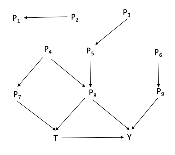
In our problem setting, the conditional causal effect can be reduced to a simple form as follows, given a causal DAG and $Y$’s parents.

Similarly, $\operatorname{P}(y\mid do(T=0),\mathbf{P})=\operatorname{P}(y\mid do(T=0),\operatorname{PA}^{\prime}(Y)=\mathbf{p^{\prime}})$.

Therefore, the lemma is proved. $\Box$

The above lemma reduces the conditional set from all pretreatment variables to the parents of $Y$ excluding $T$. The following theorem shows how the conditional causal effect of $T$ on $Y$ is estimated in our problem setting.

In DAG $G_{\underline{T}}$ where outgoing edges of $T$ have been removed, $\operatorname{PA}^{\prime}(Y)$ $d$-separate nodes $T$ and $Y$, and hence $Y\mathbin{\mathchoice{\hbox to0.0pt{\hbox{$\displaystyle\perp$}\hss}\kern 3.46875pt\kern 3.46875pt\hbox{$\displaystyle\perp$}}{\hbox to0.0pt{\hbox{$\textstyle\perp$}\hss}\kern 3.46875pt\kern 3.46875pt\hbox{$\textstyle\perp$}}{\hbox to0.0pt{\hbox{$\scriptstyle\perp$}\hss}\kern 2.48856pt\kern 2.48856pt\hbox{$\scriptstyle\perp$}}{\hbox to0.0pt{\hbox{$\scriptscriptstyle\perp$}\hss}\kern 1.78203pt\kern 1.78203pt\hbox{$\scriptscriptstyle\perp$}}}T\mid\operatorname{PA}^{\prime}(Y)$. Therefore, $\operatorname{P}(y\mid do(T=1),\operatorname{PA}^{\prime}(Y)=\mathbf{p^{\prime}})=\operatorname{P}(y\mid T=1,\operatorname{PA}^{\prime}(Y)=\mathbf{p^{\prime}})$ according to Rule 2 in Theorem 1. Therefore, $\operatorname{P}(y\mid do(T=1),\mathbf{P=p})=\operatorname{P}(y\mid T=1,\operatorname{PA}^{\prime}(Y)=\mathbf{p^{\prime}})$.

Similarly, $\operatorname{P}(y\mid do(T=0),\mathbf{P=p})=\operatorname{P}(y\mid T=0,\operatorname{PA}^{\prime}(Y)=\mathbf{p^{\prime}})$.

Referring to Table 2, in this case the objective functions of causal classification and uplift modelling are the same. Therefore, causal classification can be resolved by uplift modelling on the projected data set containing $(T,\operatorname{PA}^{\prime}(Y),Y)$.

Therefore, the theorem is proved.

$\Box$

The above theorem gives a covariate set for estimating conditional causal effect if we use causal heterogeneity modelling term, and gives a right variable set for uplift modelling. Condition on $\operatorname{PA}^{\prime}(Y)$, the conditional causal effect can be estimated in data, and uplift estimated in data is the conditional causal effect. In other words, the uplift is consistent with conditional causal effect in our problem setting.

In the DAG in Figure 1, for conditional causal effect estimation, only variables $P_{8}$ and $P_{9}$ are relevant since they are parent nodes of $Y$ apart from $T$. Note that, this is different from general feature selection since variables $P_{3}$ to $P_{9}$ are all correlated to variable $Y$. The correlation between two adjacent nodes may not be larger than that between two non-adjacent nodes. For example, the correlation between $P_{9}$ and $Y$ may be weaker than the correlation between $P_{4}$ and $Y$. In general feature selection, $P_{4}$ is preferred over $P_{9}$ because of its higher correlation.

Theorem 2 links causal classification with normal classification since both $\operatorname{P}(y\mid T=1,\operatorname{PA}^{\prime}(Y)=\mathbf{p^{\prime}})$ and $\operatorname{P}(y\mid T=0,\operatorname{PA}^{\prime}(Y)=\mathbf{p^{\prime}})$ can be estimated by classifiers in data.

In some applications, domain knowledge can be directly used instead of a DAG. Knowing the direct causes of $Y$ is sufficient for causal classification.

Theorem 2 and Corollary 1 establish the conditions under which causal classification can be resolved by uplift modelling. The conditions are also for unbiased estimation of conditional causal effects in data. Under the conditions, causal heterogeneity modelling and uplift modelling are consistent, and they both can be used for causal classification. Hence, in the following, we do not distinguish causal heterogeneity modelling and uplift modelling.

When we do not know the causes of $Y$, finding $\operatorname{PA}(Y)$ from data is the first step for causal classification. One straightforward way is to learn an entire causal DAG from data and then to read $\operatorname{PA}(Y)$ from the DAG, However, learning an entire DAG is computationally expensive or intractable with high dimensional data. Furthermore, it is often unnecessary and wasteful to find the entire DAG when we are only interested in the local structure around $Y$.

Local structure discovery [15, 16] fits our purpose better. Currently there are mainly two types of local structure discovery methods, one for identifying $\operatorname{PC}(Y)$, the set of Parents (direct causes) and Children (direct effects) of the target $Y$; and one for discovering $MB(Y)$, the Markov Blanket of $Y$, i.e. the parents, children and spouses (the parents of the children) of $Y$. Discovering $\operatorname{PC}(Y)$ is sufficient in our problem setting, $Y$ does not have descendants, i.e. $\operatorname{PC}(Y)=\operatorname{PA}(Y)$. Several algorithms have been developed for discovering $\operatorname{PC}(Y)$, such as MMPC (Max-Min Parents and Children) [17] and HITION-PC [18]. These algorithms use the framework of constraint-based Bayesian network learning and employ conditional independence tests for discovering $\operatorname{PC}(Y)$.

Our framework builds a causal classification model and conducts classification using the following Two Model approach.

Based on the proposed framework, we present the Causal Classification by the Two Model approach (CCTM) in Algorithm 1. The training phase of CCTM is to build two classifiers using variables in $\operatorname{PA}^{\prime}(Y)$ in the two sub data sets containing $T=1$ and $T=0$ respectively. Any classification method, such as decision tree or SVM can be plugged in to build the classifiers. In the prediction phase, the trained classifier pairs $M_{T=1}$ and $M_{T=0}$ predict whether a treatment will lead to a positive response (effect) or not. Line 1 of the prediction phase projects the test data set to contain the same variables in $\operatorname{PA}^{\prime}(Y)$ in order to use the two classifiers to estimate $\operatorname{P}(y\mid T=1,\mathbf{P^{\prime}=p^{\prime}})$ and $\operatorname{P}(y\mid T=0,\mathbf{P^{\prime}=p^{\prime}})$ respectively for an individual. If the difference in the probabilities (estimated conditional causal effect) is larger than $\theta$, the individual is predicted to have a positive response and should be treated. Otherwise, the treatment should not be applied to the individual.

In this section, we show how to use local structure learning algorithms MMPC and HITON-PC [15] to achieve the first step in the framework: to find the parents of the outcome variable. We also demonstrate their performance for parent discovery. Their implementations are from the Causal Explorer package [19], and $G^{2}$ test (with significance level 0.01) is used for conditional independence test. For the conditional independence tests, the maximum size of a conditioning variable set is 3 for both algorithms. The experiments are done on a PC with Intel(R) i5-8400 and 16GB memory.

We will use data sets which have known parents for evaluation, i.e. we use the known parents as the ground truth to evaluation the results of parent discovery. Four benchmark Bayesian networks (BNs), CHILD [20], ALARM [21], PIGS [22], and GENE [23] (www.bnlearn.com/bnrepository) containing 20, 37, 441 and 801 variables respectively, are used to generate the evaluation data sets. For each BN, we generate data sets with 500, 1000, and 5000 samples respectively. For each sample size, we generate a group of 10 data sets, so in total 120 data sets are generated for the four BNs. We make use of nodes having no descendants as the treatment or outcome variable, to be consistent with our problem setting, i.e. $T$ and $Y$ have no descendants and all other variables are pretreatment.

The quality of parent discovery is measured by the average precision, recall, and F1 score of the discovered parents against the known parents in each data set. The average precision, recall, and F1 score are reported in Table 3. In most cases, the algorithms produce accurate results. For the data sets with 5000 samples, both MMPC and HITON-PC achieve perfect results with 100% precision and recall. This shows that if the data set is large, the parent discovery can be accurate.

To show the time efficiency and scalability of the local structure learning algorithms MMPC and HITON-PC, we generate data sets with 5 K, 15 K, 25 K, 35 K and 50 K samples respectively. As shown in Figure 2, both MMPC and HITON-PC are fast and scalable to the size of data sets.

In the proposed CCTM algorithm, MMPC is used because it is slightly faster than HITON-PC.

We demonstrate the efficacy of the CCTM framework by using two instantiations of it. We use two popular classifiers, SVM and Random Forest (RF) to instantiate the proposed causal classification framework to two algorithms, denoted as CCTM-SVM and CCTM-RF respectively. The implementations of RF and SVM are from
https://cran.r-project.org/web/packages/randomForest/index.html and https://www.csie.ntu.edu.tw/~cjlin/libsvm/respectively. Default parameters are used.

We will demonstrate that the instantiated algorithms CCTM-SVM and CCTM-RF perform well in causal classification, and that Theorem 2 is generally applicable to uplift (and causal heterogeneity) modelling methods. In this evaluation, for each method, we compare its performance when using parent variables with its performance when using all variables.

To benchmark the instantiated algorithms, we also run some well known uplift (and causal heterogeneity) modelling methods, including Uplift Random Forests (Uplift RF) [24], Uplift Causal Conditional Inference Forests (Uplift CCIF) [25], t-Statistics Tree [26], CausalTree [9], and the X-Learner [11]. We also compare the instantiations with two treatment responder classification methods under causal effect monotonicity [27]: RespSVM-Linear and RespLR-Gen. In our experiments, we use the implementations of the methods from authors’ or commonly used packages: Uplift RF and Uplift CCIF from https://cran.r-project.org/web/packages/uplift/index.html, t-Stats Tree and Causal Tree from https://github.com/susanathey/causalTree, X-Learner from https://github.com/soerenkuenzel/causalToolbox, and RespSVM-Linear and RespLR-Gen from https://github.com/CausalML/classifying-responders. Default parameters are used for all methods except RespSVM-Linear and RespLR-Gen. The parameter on the regularization term for RespSVM-Linear is selected by 5-fold cross validation on each training data set from the set (0.001, 0.01, 0.1, 1, 10, 100, 1000). RespLR-Gen is a neural network with no hidden layer learning by the Adam optimiser using 200 epochs as in [27].

We will need data sets with known ground truth (true uplifts or conditional causal effects) for evaluation. Two groups of simulation data sets (Group 1 and Group 2) are generated following the work in [28]. The generation program is at https://cran.r-project.org/web/packages/CovSelHigh/index.html. The causal DAGs used for generating the data sets are shown in Figure 3. Each group contains 10 data sets, and each data set has 10,000 samples and 102 variables. $T$ and $Y$ are binary. Apart from $X_{1}$ to $X_{10}$ in the DAGs, other 90 variables which are irrelevant to $T$ and $Y$ are included to simulate real world situations. 100 variables are drawn from a mixture of continuous and binary distributions. where the left graph (for generating Data set 1) is to simulate the situation when causal sufficiency is satisfied, and the right graph (for generating Data set 2) is to simulate the situation when hidden variables exist. When generating a data set in Group 2, after obtaining the data set based on the right structure in Figure 3, we remove the columns for variables $U_{1}$,$U_{2}$ and $U_{3}$ from the data set to simulate latent variables. The DAG underlying Group 2 data sets does not cause a major problem for the CCTM methods although the casual sufficiency assumption is not satisfied. In the DAG, the two paths with hidden variables do not link to $T$ and hence hidden variables do not cause a bias in causal effect estimation. $X_{4}$ is not a parent of $Y$ but is a good proxy of $U_{3}$ (which is the parent of $Y$). Some effect of $U_{2}$ on $Y$ (not via $X_{9}$) is missed, and this results in an uncertainty for all methods.

For evaluation of causal classification, a half of data set is used for training models and another half is used to test the accuracy. Threshold $\theta$ is set to 0 to separate positive causal effect from zero or negative causal effect. A prediction is correct if the treatment assignment is the same as the assignment based on the ground truth causal effect for data generation.

The accuracies of all methods are presented in Table 4. Each method is run by using all variables and $\operatorname{PA}^{\prime}(Y)$ respectively and the two accuracies are compared. T-test is conducted with the null hypothesis that there is no difference between two accuracies achieved using all variables and $\operatorname{PA}^{\prime}(Y)$. The confidence level of the t-test is set at 95%, and significant results are marked by *. Using parent variables consistently achieves higher accuracy than using all the variables for all methods. Most differences are statistically significant. This means that our theoretical result, i.e. Theorem 2, improves all uplift (causal heterogeneity) modelling methods.

Table 5 presents the results of t-tests of accuracies between a pair of a CCTM method and a comparison method. Using off-the-shelf package without parameter tuning, the two instantiations achieve mostly better performance in comparison with other methods (17/28). They perform worse than other in three cases. Considering that the comparison methods are tailor designed (some are asymptotic) solutions, the performance CCTM methods is very good.

We evaluate CCTM-RF and CCTM-SVM by benchmarking with those uplift (causal heterogeneity) modelling methods in two real world data sets, Hillstrom [29] and Twins [30]. In this evaluation, the estimated uplifts (conditional causal effects) are not dichotomised and the capability for identifying subgroups with largest uplifts (causal effects) is evaluated.

Hillstrom contains 42613 customer records from an email marketing campaign collected for an uplift modelling challenge [29]. Half of these customers were randomly chosen to receive an advertisement email targeting male users, and the other half of the customers served as a control group. There are 7 pretreatment variables describing customers. The outcome is whether a customer visits the website. MMPC finds three parent variables for the outcome.

Twins [30]consists of 4821 samples of twin births (with birth weight $<2$ Kg and having no missing values) in the USA between 1989 and 1991. Each record contains 40 pretreatment variables. describing biological parents, pregnancy and information about the birth. Treatment $T\!=\!1$ indicates the heavier one in the twins and $T\!=\!0$ indicates the lighter one. The outcome is the mortality of a child after one year. MMPC finds 4 parent variables for the outcome.

Since there are not ground truth uplifts (or conditional causal effects), we use the Qini curve [31], a widely used metric for uplift modelling to compare the algorithms. Qini coefficient is calculated as $n_{Y=1,T=1}-(n_{Y=1,T=0}\cdot n_{T=1})/(n_{T=0})$, where $n_{Y=1,T=1}$ and $n_{Y=1,T=0}$ are the numbers of positive outcomes in the treatment ($T=1$) and control ($T=0$) groups respectively, and $n_{T=1}$ and $n_{T=0}$ are the total numbers of samples in the treatment and control groups respectively. Qini curve shows the cumulative amount of the uplift as a function of the proportion of test samples treated in descending order of predicted uplifts (conditional causal effects). The larger the area a curve covers, the better the corresponding method is. A 10 fold cross validation is used to obtain the Qini curve for each method, and parameter selection is as discussed before.

Figure 4 shows that the CCTM instantiations, CCTM-SVM and CCTM-RF, achieve competitive performance with other compared methods, ranked the second and third with the Hillstrom data set, and the third and first with the Twins data set. This means that CCTM can also work for uplift (causal heterogeneity) modelling where continuous uplifts (conditional causal effects) are used instead of dichotomised uplifts (conditional causal effects).

In sum, the experimental results demonstrate that the proposed framework works with off-the-shelf methods. Parent discovery is essential in our framework and Section 5.2 shows that it is helpful for existing uplift (causal heterogeneity) modelling methods too. For both causal classification and uplift (causal heterogeneity) modelling tasks, the two CCTM instantiations perform competitively in comparison with other methods. Note that, the purpose of these experiments are not to demonstrate which methods are better than the others, but to show that the proposed framework can be instantiated using off-the-shelf methods and can achieve competitive performance with other existing methods. The framework is principally correct when assuming causal sufficiency, and provides a means for users to implement any causal classification methods fitting their applications.

We are aware of the criticisms on two model approach in [32], but the recent surveys and evaluations [6, 8, 33] have shown that a two model method performs competitively with other methods. In some cases, a two model method performs the best. However, the conditions for using a two model method have not be discussed in the previous work, and what we have done in this paper has filled in the gap. The proposed framework supports a number of choices of uplift (causal heterogeneity) modelling methods from the off-the-shelf supervised methods for an application, and users can choose the most suitable one for their application.

Parent identification is a crucial step for the CCTM framework. If other variables are pretreatment variables and a data set is reasonably large, in our experience, parent discovery is quite accurate. Furthermore, Corollary 1 enables domain experts to review the automatically discovered parents. In case of missing parents or inclusion of false parents, they have different impacts on the causal classification models. In the case of missing parents, some confounding variables may be missed, and this will lead to a bias in conditional causal effect estimation. When false parents are included, false inclusion may introduce high variance in estimation. Both lead to inaccurate models in causal classification.