Spontaneous vectorization in the presence of vector field coupling to matter
Abstract
We examine the possibility of spontaneous vectorization in the vector-tensor theories with the vector conformal and disformal couplings to matter. We study the static and spherically symmetric solutions of the relativistic stars with the nontrivial profile of the vector field satisfying the boundary conditions at the spatial infinity, where represents the vector field. First, we study the linear perturbations about the general relativistic (GR) stellar solutions with the vanishing vector field . We show that the pure vector disformal coupling causes the ghost or gradient instability of the GR stars, indicating the breakdown of the hyperbolicity on the GR stellar backgrounds. On the other hand, the pure conformal coupling causes the tachyonic instability of the GR solutions and would lead to the spontaneous growth of the vector field toward the nontrivial solutions as in the manner of spontaneous scalarization in the scalar-tensor theories. We then construct the static and spherically symmetric solutions of the relativistic stars with and nodes of the vector field in the presence of the pure disformal coupling. We find that the properties of the solutions with the nontrivial vector field are similar to those of the generalized Proca theories. As in the mass-radius diagram the branches of the and node solutions are disconnected to that of the GR solutions in the lower density regimes, they may be formed from the selected choice of the initial conditions. We also construct the node solutions in the case of the pure conformal coupling, and show that the branch of these solutions is connected to that of the GR solutions in both the low and high density regions and hence would arise spontaneously via the continuous evolution from the GR solutions. Finally, we briefly discuss the combined effects of the conformal and disformal couplings on the nontrivial solutions.
I Introduction
It is well-known that general relativity (GR) has passed all experimental tests from the Solar System to the strong-field and low-velocity regime of binary pulsars Will 2014. With the dawn of gravitational-wave astronomy, a new frontier for testing GR in strong-field and high-velocity regimes has opened Berti et al. 2015; Berti et al. 2018a; Berti et al. 2018b. Some of the scalar-tensor theories of gravitation not only pass the Solar System tests, but also allow for large deviations from GR in the relativistic star interiors such as neutron stars, through the process called spontaneous scalarization Damour and Esposito-Farèse 1993. Spontaneous scalarization would be triggered by the tachyonic growth of the scalar field inside the relativistic stars. In the simplest case where the metrics in the Jordan and Einstein frames are related by the conformal transformation, , the GR solution with the vanishing scalar field suffers from the tachyonic instability if , leading to the relativistic stars with the nontrivial profile of the scalar field Damour and Esposito-Farèse 1996; Harada 1997; Harada 1998; Novak 1998; Palenzuela et al. 2014; Sampson et al. 2014; Pani and Berti 2014; Silva et al. 2015. For the exponential coupling , spontaneous scalarization of the static and spherically symmetric stars happens for Harada 1997; Harada 1998, depending weakly on the equation of state and fluid properties Novak 1998; Silva et al. 2015.
An interesting question is whether phenomena similar to spontaneous scalarization can be induced by another field, for instance, the vector field. The possibility of spontaneous vectorization triggered by the tachyonic instability of the vector field has been recently studied in Refs. Ramazanoğlu 2017; Ramazanoğlu 2019; Annulli et al. 2019; Ramazanoğlu and Ünlütürk 2019; Kase et al. 2020. The authors of Ref. Annulli et al. 2019 have studied the model of the vector-tensor theory with the nonminimal couplings to the Ricci tensor (as well as ), and found that below the threshould couplings the GR solutions with the vanishing vector field suffer from the tachyonic instability. They have also constructed the static and spherically symmetric solutions with the nontrivial vector field profile with nodes for , which would be formed from the selected choice of the initial conditions, rather than from the tachyonic instability of the GR solutions. A similar model in the context of the generalized Proca theories Heisenberg 2014; De Felice et al. 2016 with the nonminimal coupling to the Einstein tensor , which is free from the Ostrogradsky instability, has been studied in Ref. Kase et al. 2020. The node solutions have been shown to exhibit the similar behavior to those in the above model, and the node solutions have also been studied. While the coupling parameter for the existence of the node solutions is consistent with the instability of the GR solutions, in the mass-radius diagram the branch of the nontrivial vector field solutions is not smoothly connected to that of the GR solutions with the vanishing vector field. Thus, it may be formed from the selected choice of the initial conditions as the node solutions. These properties of the relativistic stars were much different from those of spontaneous scalarization.
While these studies have analyzed the possibility of spontaneous vectorization from the viewpoint of the Jordan frame where the nonminimal coupling of the vector field to the spacetime curvature is present, the other approach is to take the viewpoint of the Einstein frame where the nonminimal coupling of the vector field to matter is present. Ref. Ramazanoğlu 2017 has shown that the conformal coupling to the vector field , where
| (1) |
is the norm of the vector field and is the regular function of , could trigger the tachyonic instability of the vector field, and the explicit stellar solutions with the nontrivial profile of the vector field have been constructed for the coupling () and the nonzero mass of the vector field. More recently, Ref. Ramazanoğlu and Ünlütürk 2019 has also suggested that the vector disformal coupling Kimura et al. 2017, , where is also the regular function of , could also trigger the tachyonic instability of the vector field in the relativistic stars. We note that the Jordan frame formulation of the case of the pure conformal coupling was recently presented in Ref. Ramazanoğlu 2019. We also note that in the context different from spontaneous vectorization hairy relativistic star solutions in generalized vector-tensor theories have been recently studied in Refs. Chagoya et al. 2017; Kase et al. 2018.
The purpose of the paper is to present the more quantitative study of the relativistic stars with the nontrivial profile of the vector field in the presence of conformal and disformal couplings to matter, and to address whether the solutions satisfying the boundary conditions at the spatial infinity can be the vectorized solutions of the relativistic stars. In this paper, we consider the vector-tensor theory with the direct coupling of the vector field and matter, whose action is given by
| (2) | |||||
where with being the gravitational constant and being the speed of light, is the metric in the Einstein frame, is the scalar curvature associated with , is the vector field, is the field strength, and is the bare mass squared of the vector field. We assume that the metric in the Jordan frame denoted by is related to the Einstein frame one by the combination of conformal and disformal couplings
| (3) |
The gravitational part of the action in Eq. (2) written in terms of the Jordan frame metric belongs to a class of the beyond-generalized Proca theories Heisenberg et al. 2016a; Heisenberg et al. 2016b; Kimura et al. 2017. In this paper, we will work in the units where the speed of light to be unity , unless it should be shown explicitly.
For the analysis of the solutions of the relativistic stars, we will employ only the polytrope equation of state Damour and Esposito-Farèse 1993; Baumgarte and Shapiro (See Eqs. (51) and (54)). Since this equation of state would be less realistic, we will not make any comparison with the observational data associated with the mass and radius of the neutron stars, and focus on the physical properties of the solutions. In Ref Kase et al. 2020, it has also been shown that the qualitative features of the relativistic stars in the generalized Proca theories do not depend on the choice of the equations of state. We expect that in our model the properties of the star are also less sensitive to the choice of the equation of state.
The organization of the paper is as follows: In Sec. II, we will derive the set of the covariant equations of motion by varyng the action (2) and analyze the stability of the GR solutions. In Sec. III, we will apply the above formulation to the static and spherically symmetric spacetme, reduce the set of the equations of motion to the modified Tolman-Oppenheimer-Volkov system, and derive the interior and exterior solutions of the star. In Sec. IV, we will analyze the properties of the test vector field on top of the constant density star, and estimate the typical values of the conformal and disformal couplings to enhance the vector field at the center of the star. In Sec. V, we will explicitly construct solutions of the relativistic star with the nontrivial vector field profile in the simplest model of the pure disformal coupling and discuss their properties. In Sec. VI, we will analyze the simplest model with the pure conformal coupling. In Sec. VII, we will briefly discuss the combined effects of the conformal and disformal couplings on the nontrivial solutions. The last Sec. VIII will be devoted to a brief summary and conclusion.
II the vector-tensor theories and the GR solutions
In this section, we derive the covariant equations of motion by varying the action (2) with respect to the Einstein frame metric and the vector field .
II.1 The covariant equations of motion
Varying the action (2) with Eq. (3) with respect to the vector field , we obtain the equation of motion for the vector field
| (4) |
where , and we have defined the energy-momentum tensor of matter in the Jordan frame
| (5) |
with the inverse and determinant of the metric tensor in the Jordan frame Eq. (3), respectively, given by Eq. (A). On the other hand, varying the action (2) with respect to the Einstein frame metric , we obtain the gravitational equations of motion in the Einstein frame
| (6) |
where we have defined the energy-momentum tensor of the vector field and matter in the Einstein frame, respectively by
| (7) | |||||
and
| (8) | |||||
with , , and . Acting on Eq. (6), with the use of the contracted Bianchi identity , we find
| (9) |
which after some algebra leads to
| (10) | |||||
II.2 The GR solutions and their stability
The metric satisfying the Einstein equations in GR
| (11) |
and the vanishing vector field (and hence ) are the solution of the theory (2) with Eq. (3) for the coupling functions and are regular at and , which can be written in terms of the Taylor series with respect to ,
| (12) | |||||
| (13) |
where () and () are constants. For the couplings (12) and (13) regular at , substituting into Eqs. (3), (7), and (8), we find that
| (14) |
Eq. (6) reduces to the ordinary Einstein equation (11) and Eq. (II.1) is trivially satisfied. This is the GR solution.
We then consider the small perturbations about the GR solutions with . At the level of the linear perturbations, the equations for the metric and vector field perturbations are decoupled. Thus, the metric perturbation obeys the perturbed Einstein equation in GR,
| (15) |
where and are the perturbed Einstein and energy-momentum tensor of matter, respectively. From Eq. (II.1), the vector field perturbation satisfies
where is the perturbed field strength.
We assume the perfect fluid form of the matter energy-momentum tensor , where is the four-velocity satisfying . We also assume a general static and spherically symmetric solution whose metric is given by
where and are functions of , is the metric of the unit two-sphere, and the indices run the directions of the two-sphere. In the static and spherically symmetric spacetime Eq. (II.2), only the - and -components of the vector field can have nonzero values
| (18) |
with .
We focus on the radial perturbations where the vector field perturbation is explicitly given by
| (19) |
We note that for the nonradial perturbations with the multipole indices , because of the centrifugal term proportional to , the effective potential is always enhanced, and hence to discuss the stability of the GR solutions it is sufficient to discuss the radial perturbations. In the static GR background (II.2) with and , at the level of the linearized perturbations we obtain
| (20) | |||||
| (21) |
where the prime denotes the derivative with respect to , , and we have defined
| (22) | |||||
| (23) |
Combining Eqs. (20) and (21), we obtain the master equation for the vector field perturbation about the background
| (24) |
In the case of the pure vector conformal coupling and , and for the tachyonic instability would take place for even for . The tachyonic instability suggests that the GR solution would spontaneously evolve to the nontrivial solution with the nonzero value of the vector field, which would be energetically more stable. In Sec. VII, we will construct the nontrivial solutions for the massless case as the possible consequence of the tachyonic instability.
On the other hand, in the case of the pure vector disformal coupling and , and , and hence especially for the massless case , we have , irrespective of the sign of . This suggests that the GR solution would suffer from the ghost or gradient instability, rather than the tachyonic instability. This instability would be related to the breakdown of the hyperbolicity on the GR stellar backgrounds, rather than the mere energetic instability. Thus, the pure disformal coupling would not cause spontaneous vectorization as in the way analogous to spontaneous scalarization. The result is rather different from the expectation in Ref. Ramazanoğlu and Ünlütürk 2019 that the disformal coupling to the matter would also cause the tachyonic instability on the GR stellar background. Nevertheless, in Sec. VI, we will explicitly construct the solutions of the relativistic stars with the nontrivial profile of the vector field, as they may be formed via the initial conditions different from the GR solutions with . We will explicitly confirm that in the mass-radius diagram the branches of the nontrivial solutions are disconnected to that of the GR solutions.
III Static and spherically symmetric spacetime
In this section, we focus on the static and spherically symmetric spacetime (II.2) and (18), and derive the equations to analyze the hydrostatic structure of the relativistic stars, i.e., the modified Tolman-Oppenheimer-Volkoff equations.
III.1 The modified Tolman-Oppenheimer-Volkoff equations
We assume that the nonzero components in the Jordan frame (3) are given by the perfect fluid form
| (25) |
Correspondingly, the nonzero components of the energy-momentum tensor of matter in the Einstein frame are given by Eq. (A).
The -component of the vector field equation (II.1) is given by
| (26) |
which allows the two branches, or the combination inside the round bracket vanishes. Here, we choose the former branch , and then the Jordan frame metric Eq. (A) reduces to the diagonal form and the energy-momentum tensor of matter in the Einstein frame also has the perfect fluid form whose components are given by Eq. (74).
The -component of the vector field equation of motion (II.1) is given by
| (27) |
On the other hand, the -, -, and - components of the gravitational equations of motion (6) are respectively given by
| (28) | |||
| (29) | |||
| (30) |
Finally, the nontrivial -component of Eq. (10) is given by
| (31) | |||||
Eliminating with the mass function defined by
| (32) |
Eqs. (28) and (29) can be rewritten as
| (33) | |||||
| (34) | |||||
Eq. (31) is rewritten as
| (35) | |||||
Similarly, eliminating , Eq. (27) reduces to
| (36) | |||||
We focus on matter with the isotropic pressure
| (37) |
and then all the unknown are the five variables , , , , and , while we have the four independent equations Eqs. (33), (34), (35), and (36). The system of the equations is closed once the equation of state
| (38) |
is specified. We note that Eq. (30) is not independent of the other equations.
III.2 The interior solution
The interior solution is obtained by integrating Eqs. (33), (34), (35), and (36) with a given equation of state (38) from the center of the star to the surface of the star whose position is determined by the condition (See Eq. (74))
| (39) |
The interior solution in the vicinity of the center is given by
| (40) |
where the coefficients , , , and are given in Eq. (A), with , , , , and in these relations. Without loss of generality, we set , so that the time coordinate corresponds to the proper time at the center of the star. From Eq. (A), the case of , , and recovers the stellar solution in GR
| (41) |
From Eq. (A) with , we find the relation of the mass functions and radial coordinates of the Jordan and Einstein frames, where , and respectively given by
| (42) | |||||
| (43) |
Thus, the radius of the star in both the frames is related by
| (44) |
We assume that as , , , and is regular, and then the masses in both the frames coincide
| (45) |
III.3 The external solution and the matching at the surface of the star
From now on, we set . The external solution is then given by the Reissner-Nordström solution
| (46) |
where , , , and are integration constants. The external solution is matched to the internal one at the surface of the star determined by Eq. (39). Imposing the continuity of , , and at ,
| (47) |
we obtain
| (48) |
and correspond to the mass and vector field charge of the star. Since the gauge invariance is broken because of the vector field coupling to matter, is also a physical quantity. The proper time measured at the spatial infinity is given by . The redshift factor for photons radially traveling from the center of the star to the spatial infinity is given by
| (49) |
where and are the frequencies measured at the center of the star and at the spatial infinity, respectively. Similarly, the redshift between the surface of the star and the spatial infinity is given by
| (50) | |||||
where represents the frequency measured at the surface of the star.
III.4 The polytrope equation of state
For the numerical analyses in Secs. V, VI, and VII, we employ the polytrope equation of state
| (51) |
where is the rest mass density with and being the baryonic mass and the number density, respectively, and and are constants. The mean baryonic mass is identified with the neutron mass .
The total energy density is given by , where is the dimensionless internal energy per unit mass. For adiabatic nuclear matter, the first law of thermodynamics reduces to . With and , the first law leads to , which with Eq. (51) can be integrated as . Thus, the relation between the total energy density and pressure in the Jordan frame is given by
| (52) |
Defining the dimensionless number density by , with and being the mean number density of the baryonic particles, the total energy density and pressure can be written as
| (53) |
where . Eq. (52) can be rewritten in terms of
| (54) |
For our numerical analyses, we will choose the parameters
| (55) |
We also parametrize the pressure at the center of the star () as
| (56) | |||||
where represents a constant parameter. Correspondingly, from Eq. (54) then the energy density at the center of the star is given by
| (57) |
IV The test vector field solutions in the weak gravity regimes
Before going to the numerical studies with the polytrope equation of state (51) and (54) in the next sections, we estimate the critical vector field couplings that enhance the amplitude and charge of the test vector field on top of the constant density star in GR.
For any regular coupling (12), the GR stellar solution with exists in the vector-tensor theory (2) with Eq. (3). Since there is no distinction between the Jordan and Einstein frames, , and . We consider an incompressible fluid, , where the interior metric and pressure () are given by
| (58) |
where at the surface of the star , , and and are the total mass and compactness
| (59) |
The exterior solution () is given by the Schwarzschild metric
| (60) |
On top of the constant density star, the test vector field obeys the equation
| (61) | |||||
Thus, in the weak gravity regime , the approximated interior solution () is given by
| (62) |
where we have chosen the regularity boundary conditions at the center of the star , for which the solution decreases. We assume that
| (63) |
We note that for , the interior solution regular at the center of the star grows as , which is unphysical and excludes this possibility in the rest.
The exterior solution () is given by
| (64) |
The matching of Eqs. (62) and (64) at the surface of the star provides
| (65) |
As , and are enhanced for the case
| (66) |
where denotes the number of nodes of the vector field inside the star. The estimation above is analogous to the case of spontaneous scalarization Harada 1997.
Here, we focus on the fundamental node solutions . Extrapolating to the relatively high compact star , the value of the coupling for which the vector field is amplified is given by . If the above static solution becomes the weak field approximation for the fully vectorized relativistic stars, it implies that the full vectorized solution would exist for or to be of .
V The case of the pure disformal coupling
In this section, we consider the simplest model with the pure disformal coupling given by
| (67) |
where is the constant. From Eqs. (44) and (45), we obtain
| (68) |
As argued in Sec. II.2, the pure disformal coupling induces the ghost or gradient instability of the GR solutions, rather than the tachyonic instability. Thus, the hyperbolicity of the perturbations is broken on the GR stellar background and hence spontaneous vectorization analogous to spontaneous scalarization would not take place. Nevertheless, we will study the nontrivial solutions satisfying the boundary condition , as they may be formed from another choice of the initial conditions. As we will see below, the properties of the solutions are similar to those obtained in the generalized Proca theories Kase et al. 2020.
V.1 The node solutions
First, we focus on the node solutions, where the temporal component of the vector field never crosses both the interior and exterior of the star. In Fig. 1, the typical behavior for the node solutions is shown for . In both the panels, the solid and dashed curves correspond to the cases of and , respectively. In the top panel, the red and blue curves represent the energy density and pressure inside the star, respectively, and the horizontal and vertical axes are shown in the units of and , respectively. The bottom panel shows the temporal component of the vector field as the function of . In the bottom panel, the red points correspond to the surface of the star.


In Fig. 2, following Eq. (III.3), is shown as the function of for . The red, blue-dashed, green-dotted, and black-dotdashed curves correspond to the cases of , respectively.

All the curves take at , which corresponds to the GR solutions. The curves for take the positive values for the smaller , and then cross the axis of once, where the node solutions exist. On the other hand, the curve for never crosses the axis of except at and hence there exists only the GR solutions. As , i.e., , increases, the root of becomes smaller and finally reaches the origin . Thus, above the critical value of , the node solutions converge to the GR solutions with .
In Fig. 3, the mass-radius diagram is shown for the node solutions. In the top panel, the red, blue-dashed, and green-dotted curves correspond to the cases of , respectively, while the black curve corresponds to the GR solutions. The bottom panel focuses on the case of . In the bottom panel, the black-dashed curve represents the range of the branch of the GR solutions for which the branch of the node solutions coexists. The radius and mass are measured in the units of and the Solar mass , respectively.
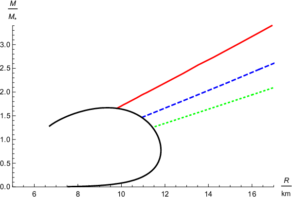
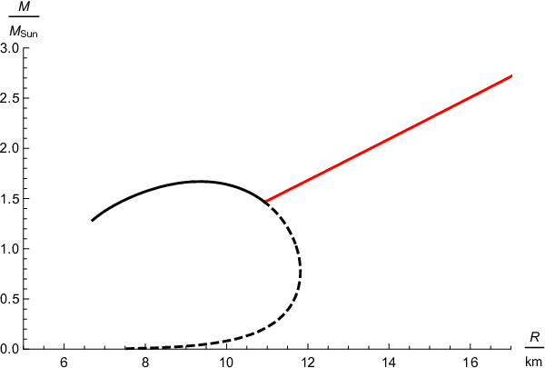
As , i.e., , decreases, both the mass and radius increase. On the other hand, as increases, the branch of the nontrivial vector field solutions finally converges to that of the GR solutions.
For , the node solutions exist only for . The similar behavior was also observed in the generalized Proca theories Kase et al. 2020. In our model, as suggested in Sec. II.2, the node solutions arise from the selected choice of the initial conditions rather than the instability of the GR solutions, as the hyperbolicity of the perturbations would be broken on the GR stellar backgrounds.
V.2 The node solutions
Next, we focus on the node solutions. In Fig. 4, the typical behavior for the node solutions is shown for . In both the panels, the solid and dashed curves correspond to the cases of and , respectively. In the top panel, the red and blue curves represent the energy density and pressure inside the star, respectively, and the horizontal and vertical axes are shown in the units of and , respectively. The bottom panel shows the temporal component of the vector field as the function of . In the bottom panel, the red points correspond to the surface of the star.


In Fig. 5, is shown as the function of for . The red-dashed, blue-dotted, green-dotdashed, and black curves correspond to correspond to the cases of , respectively.

For the smaller , i.e., , as shown by the red curve, there is no root satisfying , which corresponds to the node solutions. For the larger , i.e., , as shown by the blue and green curves, two roots of appear at the finite . As further increases, the smaller root approaches and finally converges to the GR solutions , while the larger root keeps increasing. For the sufficient large , only the larger root exists. As in Ref. Kase et al. 2020, we focus on the smaller root and show the mass-radius diagram.
In Fig. 6, the top panel shows the mass-radius diagram for the node solutions. The red, blue-dashed, and green-dotted curves correspond to the cases of , while the black curve corresponds to the GR solutions. The bottom panel shows the solution for . In the bottom panel, the black-dashed curve represents the range of the branch of the GR solutions for which the branch of the node solutions coexists. The radius and mass are measured in the units of and the Solar mass , respectively.


In the bottom panel, for the smaller values of , i.e., smaller , the solution is described by the GR solution with the polytrope equation of state, and across the critical central pressure , it suddenly jumps to the nontrivial node solutions described by the red curve. As further increases, the radius increases but the mass decreases, and the branch of the node solutions finally converges to that of the GR solutions at .
For , we observe that the node solutions exist for . The behavior of the node solutions is also similar to what was observed in Ref. Kase et al. 2020. As seen in Fig. 6, in the low density regimes the branch of the node solutions is disconnected to the branch of the GR solutions. This indicates that the node solutions may also be formed from the selected choice of the initial conditions. Although we have not employed the more realistic equations of state, we expect that the essential results are insensitive to the choice of the equations of state.
VI The case of the pure conformal coupling
We then consider the model with the pure conformal coupling given by
| (69) |
where is the constant. The relation of the mass and radius of the star in both the frames is given by Eqs. (44) and (45), respectively. We then focus on the solutions satisfying the boundary condition . As we have seen in Sec. II.2, these solutions may be formed as the consequence of the tachyonic instability of the GR solution. In this section, we focus only on the node solutions, as they can be obtained for , which is the value suggested from the analysis of the weak gravity limit in Sec IV. While the model with the massive vector field was analyzed in Ref. Ramazanoğlu 2017, we will focus on the model of the massless vector field . To our knowledge, there has been no quantitative study even in the massless case yet.
In Fig. 7, the typical behavior for the node solutions is shown for . In both the panels, the solid and dashed curves correspond to the cases of and , respectively. In the top panel, the red and blue curves represent the energy density and pressure inside the star, respectively, and the horizontal and vertical axes are shown in the units of and , respectively. The bottom panel shows the temporal component of the vector field as the function of . In the bottom panel, the red points correspond to the surface of the star.


In Fig. 8, following Eq. (III.3), is shown as the function of for (the top panel) and (the bottom panel). In the top panel, the black, red-dashed, blue-dotted, and green-dotdashed curves correspond to the cases of , respectively. In the bottom panel, the black, red-dashed, blue-dotted, and green-dotdashed curves correspond to the cases of , respectively.


In both the panels, all curves take at , which correspond to the GR solutions. For , the curves of cross the axis of at which corresponds to the nontrivial node solutions, while the curve of has no root other than . As , i.e., , increases, the root of increases, then decreases and finally converges to the GR solutions . Thus, the nontrivial node solutions exist in the intermediate range of , and in the low and high density regimes they converge to the GR solutions.
On the other hand, for , the curve of crosses the axis of once at . The curves for cross the axis of twice. The smaller root exists only for , and at the certain converges to the branch of the GR solutions. The larger root keep increasing for the increasing . Thus, the behavior for is qualitatively different from the cases of , and especially the low density regimes the -node solutions are not smoothly connected to the GR solutions.
In Fig. 9, the mass-radius diagram for the node solutions is shown. The red, blue-dashed, green-dotted, and purple-dotdashed curves correspond to the cases of the -node solutions for , respectively, while the black curve corresponds to the case of the GR solutions. The radius and mass are measured in the units of and the Solar mass , respectively.

For , the branch of node solutions is connected to the branch of the GR solutions. Thus, as in the case of spontaneous scalarization, in the mass-radius diagram, the branch of the node solutions bifurcates from the branch of the GR solutions in the low density regimes. After the significant deviations from the branch of the GR solutions, they finally merge to the GR solutions in the high density regimes. For the same radius of the star, the mass of the star for node solutions becomes smaller than that for the GR solutions. On the other hand, for the branch of the -node solutions is disconnected to the branch of the GR solutions in the low density regime, while it marges to the branch of the GR solutions in the high density regimes. For such a case, spontaneous vectorization would not happen in the same manner as spontaneous scalarization. We note that our study is the first one which shows the mass-radius diagram for the vectorized relativistic stars in the case of the massless vector-tensor theories.
In Fig. 10, the dimensionless ratio is shown as the function of the mass . The black and red-dashed curves correspond to the cases of , respectively. The mass is measured in the units of the Solar mass .

Since vectorized solutions with two different masses can share the same radius, in some range of the mass the dimensionless ratio also becomes the multivalued function of . The dimensionless ratio exceeds unity around its maximal value and approaches zero at the both endpoints, as the vectorized branch approaches the GR branch in the low and high density regimes. The maximal value of also increases as increases.
Although we have focused on the simplest model (69), we expect that spontaneous vectorization would still take place for the more general couplings (12) with and (). While the behavior in the vicinity of the bifurcation points from the branch of the GR solutions in the low and high density regimes in the mass-radius diagram would remain the same, the behavior in the intermediate density regime would depend crucially on the choice of the coupling function . The case of the other coupling function and the inclusion of the nonzero bare mass of the vector field will be left for the future work.
VII The case of the combined conformal and disformal couplings
Before closing this paper, we briefly discuss the case of the combined effects of the conformal and disformal couplings on the nontrivial solutions. For simplicity, we consider the minimal extension of the models considered in Secs. V and VI,
| (70) |
For a fixed nonzero value of where we have obtained the vectorized solutions with nodes for in Sec. VI, we will see how adding the nonzero value of modifies the structure of the nontrivial solutions and the existence of the solutions.
In Fig, 11, is shown as the function of for and . In the top panel, the black, red-dashed, blue-dotted, and green-dotdashed curves correspond to the cases of , respectively. In the bottom panel, the black, red-dashed, blue-dotted, and green-dotdashed curves correspond to the cases of , respectively.


For , the solution of corresponds to the solution with nodes as for . For , there is no solution of . For and , there are the 0-node solutions, but as seen in Fig. 12, the profile of the vector field possesses a spike inside the star.


The solution of for corresponds to a -node solution with a single spike inside the star. For these spiky solutions, as in the top panel of Fig. 12, both the energy density and pressure increase in the vicinity of the center of the star.
Thus, adding the disformal coupling to the pure conformal coupling makes the properties of the nontrivial solutions more unphysical than in the case of the pure conformal coupling. In other words, the model with the pure conformal coupling would be the most competitive one for spontaneous vectorization.
VIII Conclusions
In this paper, we have examined the possibility of spontaneous vectorization in the vector-tensor theories with the vector conformal and disformal couplings to matter given by the action Eq. (2) with (3). In each class of the couplings, we have constructed the static and spherically symmetric solutions of the relativistic stars with the nontrivial profile of the vector field satisfying the boundary conditions at the spatial infinity, . We have worked from the viewpoint of the Einstein frame, and note that the gravitational action (2) rewritten in terms of the Jordan frame metric belongs to a class of the beyond-generalized Proca theories.
First, we have considered the general couplings which allow the general relativistic (GR) solutions. After varying the action, we have derived the covariant equations of motion. Then, applying to the static and spherically symmetric spacetime, we have derived the modified Tolman-Oppenheimer-Volkoff equations. The radial component of the vector field equation forces us to set the radial component of the vector field to zero, . In the case that the bare mass of the vector field is zero, the exterior solution is given by the Reissner-Nordström solution. The external solution is matched to the internal solution constructed by solving the modified Tolman-Oppenheimer-Volkoff equations from the center to the surface of the star under the regularity boundary conditions at the center of the star. The matching at the surface of the star determines the mass and the vector field charge of the star.
After deriving the covariant equations of motion, we have investigated the linear perturbations about the static and spherically symmetric GR solutions. Focusing on the radial perturbations, we have found that the vector conformal and disformal couplings cause different kinds of instability. In the case of the pure conformal coupling, we have shown that the GR solutions suffer from the tachyonic instability, indicating that the GR solutions would spontaneously evolve to the nontrivial solutions with the nonzero value of the vector field.
On the other hand, in the case of the pure vector disformal coupling, we argued that the GR solutions suffer from the ghost or gradient instability, indicating the breakdown of the hyperbolicity on the GR stellar backgrounds. Thus, we have expected that the pure disformal coupling would not cause spontaneous vectorization in the same manner as spontaneous scalarization, and the stellar solutions with the nontrivial profile of the vector field may be formed from the selected class of the initial conditions.
Second, we have focused on the simplest model with the pure disformal coupling (67). We have constructed the static and spherically symmetric solutions with the asymptotic value . The properties of the stellar solutions are similar to those in the generalized Proca theories Kase et al. 2020. The node solutions exist for the coupling parameter of , while the node solutions exist for the coupling parameter of . As expected, in the mass-radius diagram the branch of the node solutions is disconnected to that of the GR solutions in the low density regimes.
On the other hand, we have also studied the simplest model with the pure conformal coupling (69). We have argued that the node solutions are formed spontaneously via the continuous evolution from the GR solutions. For the smaller absolute value of the conformal coupling parameter, we have found that the branch of the node solutions is connected to that of the GR solutions in the low density regimes, and hence these node solutions may be the vectorized solutions arising from the tachyonic instability of the GR solutions. The mass of the solutions is always smaller than that of the GR solutions. On the other hand, for the larger absolute value of the coupling parameter, the branch of the node solutions is disconnected to that of the GR solutions in the low density regimes, and hence the node solutions may be formed from the selected choice of the initial conditions.
We have also seen the behavior of the nontrivial solution in the presence of both the conformal and disformal couplings. Although we could obtain the nontrivial vector field solutions satisfying in this model, adding the disformal coupling to the pure conformal coupling model has made the properties of the stars more unphysical than in the case of the pure conformal coupling, as a spiky feature appears in the profile of the vector field and both the energy density and pressure increase in the vicinity of the center of the star.
While in the present work we have focused on the simplest cases of the pure vector conformal and disformal couplings with the polytrope equation of state, the analysis of the more general models with the more realistic equations of state will be left for the future studies. We will also leave the analysis of the time evolution toward the nontrivial solutions of the vector field for the future work. Clarifying these points will make the difference of the properties of spontaneous vectorization from those of spontaneous scalarization more evident.
Acknowledgements.
M.M. was supported by the research grant under the Decree-Law 57/2016 of August 29 (Portugal) through the Fundação para a Ciência e a Tecnologia, and CENTRA through the Project No. UIDB/00099/2020.Appendix A Some useful formulas
The inverse and determinant of the metric (3) are given by
| (71) |
The nonzero components of the metric in the Jordan frame in the static and spherically symmetric system are given by
| (72) |
The components of the matter energy-momentum tensor in the Einstein frame in the static and spherically symmetric system are given by
| (73) |
When , it reduces to the perfect fluid form as
| (74) | |||||
The coefficients in the approximated solutions in the vicinity of the center of the star Eq. (III.2) are given by
| (75) | |||||
References
- Will (2014) C. M. Will, Living Rev. Rel. 17, 4 (2014), arXiv:1403.7377 [gr-qc] .
- Berti et al. (2015) E. Berti et al., Class. Quant. Grav. 32, 243001 (2015), arXiv:1501.07274 [gr-qc] .
- Berti et al. (2018a) E. Berti, K. Yagi, H. Yang, and N. Yunes, Gen. Rel. Grav. 50, 49 (2018a), arXiv:1801.03587 [gr-qc] .
- Berti et al. (2018b) E. Berti, K. Yagi, and N. Yunes, Gen. Rel. Grav. 50, 46 (2018b), arXiv:1801.03208 [gr-qc] .
- Damour and Esposito-Farèse (1993) T. Damour and G. Esposito-Farèse, Phys.Rev.Lett. 70, 2220 (1993).
- Damour and Esposito-Farèse (1996) T. Damour and G. Esposito-Farèse, Phys.Rev. D54, 1474 (1996), arXiv:gr-qc/9602056 [gr-qc] .
- Harada (1997) T. Harada, Prog.Theor.Phys. 98, 359 (1997), arXiv:gr-qc/9706014 [gr-qc] .
- Harada (1998) T. Harada, Phys.Rev. D57, 4802 (1998), arXiv:gr-qc/9801049 [gr-qc] .
- Novak (1998) J. Novak, Phys.Rev. D58, 064019 (1998), arXiv:gr-qc/9806022 [gr-qc] .
- Palenzuela et al. (2014) C. Palenzuela, E. Barausse, M. Ponce, and L. Lehner, Phys.Rev. D89, 044024 (2014), arXiv:1310.4481 [gr-qc] .
- Sampson et al. (2014) L. Sampson, N. Yunes, N. Cornish, M. Ponce, E. Barausse, et al., (2014), arXiv:1407.7038 [gr-qc] .
- Pani and Berti (2014) P. Pani and E. Berti, Phys.Rev. D90, 024025 (2014), arXiv:1405.4547 [gr-qc] .
- Silva et al. (2015) H. O. Silva, C. F. B. Macedo, E. Berti, and L. C. B. Crispino, Class. Quant. Grav. 32, 145008 (2015), arXiv:1411.6286 [gr-qc] .
- Ramazanoğlu (2017) F. M. Ramazanoğlu, Phys. Rev. D96, 064009 (2017), arXiv:1706.01056 [gr-qc] .
- Ramazanoğlu (2019) F. M. Ramazanoğlu, Phys. Rev. D99, 084015 (2019), arXiv:1901.10009 [gr-qc] .
- Annulli et al. (2019) L. Annulli, V. Cardoso, and L. Gualtieri, Phys. Rev. D99, 044038 (2019), arXiv:1901.02461 [gr-qc] .
- Ramazanoğlu and Ünlütürk (2019) F. M. Ramazanoğlu and K. İ. Ünlütürk, Phys. Rev. D100, 084026 (2019), arXiv:1910.02801 [gr-qc] .
- Kase et al. (2020) R. Kase, M. Minamitsuji, and S. Tsujikawa, (2020), arXiv:2001.10701 [gr-qc] .
- Heisenberg (2014) L. Heisenberg, JCAP 05, 015 (2014), arXiv:1402.7026 [hep-th] .
- De Felice et al. (2016) A. De Felice, L. Heisenberg, R. Kase, S. Tsujikawa, Y.-l. Zhang, and G.-B. Zhao, Phys.Rev.D 93, 104016 (2016), arXiv:1602.00371 [gr-qc] .
- Kimura et al. (2017) R. Kimura, A. Naruko, and D. Yoshida, JCAP 1701, 002 (2017), arXiv:1608.07066 [gr-qc] .
- Ramazanoğlu (2019) F. M. Ramazanoğlu, Phys. Rev. D99, 044003 (2019), arXiv:1901.00194 [gr-qc] .
- Chagoya et al. (2017) J. Chagoya, G. Niz, and G. Tasinato, Class. Quant. Grav. 34, 165002 (2017), arXiv:1703.09555 [gr-qc] .
- Kase et al. (2018) R. Kase, M. Minamitsuji, and S. Tsujikawa, Phys. Rev. D97, 084009 (2018), arXiv:1711.08713 [gr-qc] .
- Heisenberg et al. (2016a) L. Heisenberg, R. Kase, and S. Tsujikawa, Phys.Lett.B 760, 617 (2016a), arXiv:1605.05565 [hep-th] .
- Heisenberg et al. (2016b) L. Heisenberg, R. Kase, and S. Tsujikawa, Phys.Rev.D 94, 123513 (2016b), arXiv:1608.08390 [gr-qc] .
- (27) T. W. Baumgarte and S. L. Shapiro, Cambridge University Press (2010) .