跳到论文正文
W Papers独立论文阅读器 arXiv:2003.11821 论文正文 计算阅读时间 · 0%
引用这篇论文根据当前论文元数据生成,正式投稿前建议核对。


License: arXiv.org perpetual non-exclusive license
arXiv:2003.11821v3 [hep-ph] 22 Jul 2020

Distinguishing Inert Higgs Doublet and Inert Triplet ScenariosPreprint: IITH-PH-0002/20

Shilpa Jangid Email: ph19resch02006@iith.ac.in, bpriyo@phy.iith.ac.in     Priyotosh Bandyopadhyay
Abstract

In this article we consider a comparative study between Type-I 2HDM and Y=0Y=0, S​U​(2)SU(2) triplet extensions having one Z2Z_{2}-odd doublet and triplet that render the desired dark matter(DM). For the inert doublet model (IDM) either a neutral scalar or pseudoscalar can be the DM, whereas for inert triplet model (ITM) it is a CP-even scalar. The bounds from perturbativity and vacuum stability are studied for both the scenarios by calculating the two-loop beta functions. While the quartic couplings are restricted to 0.1−0.20.1-0.2 for a Planck scale perturbativity for IDM, these are much relaxed (0.80.8 ) for ITM. The RG-improved potentials by Coleman-Weinberg show the regions of stability, meta-stability and instability of the electroweak vacuum. The constraints coming from DM relic, the direct and indirect experiments like XENON1T, LUX and H.E.S.S., Fermi-LAT allow the DM mass >⁣∼700, 1176\mathrel{\mathop{\kern 0.0pt\hbox to0.0pt{\raise 0.86108pt\hbox{$>$}\hss}}\lower 3.87495pt\hbox{\kern-1.90002pt$\sim$}}700,\,1176 GeV for IDM, ITM respectively. Though mass-splitting among Z2Z_{2}-odd particles in IDM is a possibility for ITM we have to rely on loop-corrections. The phenomenological signatures at the LHC show that the mono-lepton plus missing energy with prompt and displaced decays in the case of IDM and ITM can distinguish such scenarios at the LHC along with other complementary modes.

Keywords
Higgs bosons, Beyond Standard Model, Dark matter, LHC

1 Introduction

Higgs boson was the last key stone predicted by Standard Model (SM), which was discovered at the LHC Aad:2012tfa; Chatrchyan:2012xdj. So far five decay modes of the SM Higgs boson are discovered at the LHC Sirunyan:2018koj; ATLAS:2018doi and they fall nearly by SM prediction. In spite of immense success, SM cannot resolve many theoretical and experimental anomalies; like existence of dark matter (DM), explanation of very light neutrinos, Higgs mass hierarchy, vacuum stability, muon g−2g-2, etc. Though discovery of Higgs boson was a direct proof of the role of a scalar in electro-weak symmetry breaking (EWSB) the existence of other Higgs multiplets cannot be ruled out. Recent studies also show that SM stands in a metastable state Isidori:2001bm and need other scalar to make the electro-weak (EW) vacuum stable till Planck scale. This motivates to extend the SM by other Higgs multiplets.

The simplest extension could be via a singlet singletex; HiggsDM1; BLscalar but there could be a possibility of extension with another S​U​(2)SU(2) Higgs doublet, i.e. two Higgs doublet model (2HDM) 2HDMs; Honorez:2010re; HiggsDM; khan1; 2HDMpheno or with a S​U​(2)SU(2) triplet Tripletex which can enhance the vacuum stability. The extensions of SM with fermions motivated by Seesaw mechanisms often suffers from vacuum instability and one needs some extra scalar to compensate the negative effects exwfermion-Garg:2017iva. Many of these extensions have a Z2Z_{2}-odd particle, i.e. inert particle which is stable and being lightest among them, can be a dark matter candidate.

Supersymmetric sector in its minimal framework has 2HMD of Type-II primer. However, the minimal scenario is often challenged by fine-tuning of ∼125\sim 125 GeV light SM-like Higgs boson mass. One of the remedies of this problem is also to extend the Higgs sector beyond its minimal form. This can be achieved by extension by a SM gauge singlet NSSM; Bandyopadhyay:2015dio, S​U​(2)SU(2) triplet TESSM-Bandyopadhyay:2014tha or via singlet and triplet superfields TNSSM. In this case the DM particles is generated by RR-parity and it is a supersymmetric particle with odd RR-parity. The extended Higgs superfields mix at the superpotential level causing the mixing of Higgs bosons after EWSB among different representations, i.e. doublet-singlet, doublet-triplet, etc Bandyopadhyay:2015tva; dissusy; Bandyopadhyay:2015ifm; Bandyopadhyay:2017klv. However, we see the situation is very different for non-SUSY Higgs extensions, especially for the inert models. There are no mixing among these extra Higgs states and the SM particles, making them more illusive to produce and detect at the colliders. Nevertheless, they can provide the much needed dark matter candidate and also make the EW vacuum more stable.

In this article we consider two different extensions of SM to attain the dark sector. In the first one we extend SM to Type-I 2HDM with Z2Z_{2}-odd S​U​(2)SU(2) doublet that constitutes the dark sector and the scenario is known as inert Higgs doublet (IDM). In the second case we consider the dark sector as Y=0Y=0 S​U​(2)SU(2) triplet which is again Z2Z_{2}-odd and the scenario is known as inert Higgs Triplet scenario (ITM). Both the scenarios help in extending the vacuum stability 2HDMs; Tripletex; however, we will see that they differ in various constraints coming from perturbativity, vacuum stability, DM relic abundance, direct detection and collider searches. IDM has more scalar with relatively larger mass splitting among the Z2Z_{2}-odd states whereas the ITM has only two Z2Z_{2}-odd states mass degenerate at the tree-level.

Another aspect extended Higgs sector is the search for Higgs quartic coupling. The SM Higgs quartic coupling is till to be measured precisely and only bounds are obtained from the di-Higgs production constraints at the LHC Sirunyan:2018two; ATLAS:2018otd. Extended Higgs sectors have many such quartic couplings and they differ from IDM to ITM and are very crucial in determining the fate of the Higgs potential. One or few such quartic couplings can provide the much needed Higgs-DM coupling HiggsDM1; HiggsDM. In this case we focus our region where the DM mass is greater than discovered Higgs mass, i.e. 125.5125.5 GeV. Considering the bounds from vacuum stability, perturbativity, DM relic and direct DM searches we estimate the allowed parameter space and try to distinguish IDM and ITM at the LHC via the compressed spectrum and less number Z2Z_{2}-odd states for the later.

Higgs sector dark matter also has appeal as the quartic coupling between SM-like Higgs boson and dark sector is crucial in measuring such scenario experimentally as well as theoretically. There have been lots of work done in measuring Higgs-DM coupling Honorez:2010re; HiggsDM1; HiggsDM; Arina:2009um; Araki:2010zz; nevertheless a comprehensive study including bounds from vacuum stability, perturbativity, DM relic and direct DM is expected and which is the topic of this article.

This article is arranged as follows. In section 2 and section 3 we discuss the IDM and ITM briefly along with electro-weak symmetry breaking conditions and the tree-level Higgs boson masses. The comparative study of tree-level mass spectra between IDM and ITM is detailed in section 4. The perturbativity and vacuum stability bounds are discussed in section 5 and section 6 respectively. The DM relic and direct dark matter constraints are calculated in section 7 and section 8 respectively. Indirect bounds are discussed in section 9. In section 10 we dispense the parameter space verses the validity scale and in section 11 we discuss the LHC phenomenology briefly. Finally we conclude in section 12.

2 Inert Doublet Model (IDM)

The inert 2HDM is a minimalist (apart from SM singlet) extension of the SM with a second S​U​(2)SU(2) Higgs doublet Φ2\Phi_{2} with the same quantum numbers as the SM Higgs doublet Φ1\Phi_{1}. The Lagrangian is invariant under the Z2Z_{2} parity transformation where Φ2→−Φ2\Phi_{2}\rightarrow-\Phi_{2}, Φ1→Φ1\Phi_{1}\rightarrow\Phi_{1} and all the SM fields are even under this symmetry. Such discrete symmetry guarantees the absence of Yukawa couplings between fermions and the inert doublet Φ2\Phi_{2} and prohibits any tree-level flavor changing neutral currents. The most general renormalizable, CP conserving potential for inert doublet model Honorez:2010re; Gustafsson:2010zz-LopezHonorez:2006gr is given by

Vscalar\displaystyle\rm V_{scalar} =m112​Φ1†​Φ1+m222​Φ2†​Φ2+λ1​(Φ1†​Φ1)2+λ2​(Φ2†​Φ2)2+λ3​(Φ1†​Φ1)​(Φ2†​Φ2)\displaystyle=m_{11}^{2}\Phi_{1}^{\dagger}\Phi_{1}+m_{22}^{2}\Phi_{2}^{\dagger}\Phi_{2}+\lambda_{1}(\Phi_{1}^{\dagger}\Phi_{1})^{2}+\lambda_{2}(\Phi_{2}^{\dagger}\Phi_{2})^{2}+\lambda_{3}(\Phi_{1}^{\dagger}\Phi_{1})(\Phi_{2}^{\dagger}\Phi_{2}) (1)
+λ4(Φ1†Φ2)(Φ2†Φ1)+[λ5((Φ1†Φ2)2)+h.c],\displaystyle+\lambda_{4}(\Phi_{1}^{\dagger}\Phi_{2})(\Phi_{2}^{\dagger}\Phi_{1})+[\lambda_{5}((\Phi_{1}^{\dagger}\Phi_{2})^{2})+h.c],

where,

Φ1=(ϕ1+ϕ10),Φ2=(ϕ2+ϕ20)\displaystyle\Phi_{1}=\begin{pmatrix}\phi^{+}_{1}\\ \phi^{0}_{1}\end{pmatrix},\hskip 10.00002pt\hskip 10.00002pt\Phi_{2}=\begin{pmatrix}\phi^{+}_{2}\\ \phi^{0}_{2}\end{pmatrix}

and m112m_{11}^{2}, m222m_{22}^{2} and λ1−5\lambda_{1-5} are real parameters. Electro-weak symmetry breaking is achieved by giving real vev to the first Higgs doublet i.e. Φ1\Phi_{1} and the second Higgs doublet does not take part in EWSB. At EW minima,

⟨Φ1⟩=12​(0v),\langle\Phi_{1}\rangle\ =\ \frac{1}{\sqrt{2}}\left(\begin{array}[]{c}0\\ v\\ \end{array}\right), (2)

with v≃246v\simeq 246 GeV, whereas the second Higgs doublet, being Z2Z_{2}-odd, does not take part in symmetry breaking; hence the name is‘inert 2HDM’.

Using minimization conditions, we express the mass parameter m112m_{11}^{2} in terms of other parameters as follows:

m112=−λ1​v2.\displaystyle m_{11}^{2}\ =\ -\lambda_{1}v^{2}. (3)

Except for the SM Higgs boson, hh, four new physical scalar states are present: one charged Higgs boson pair H±H^{\pm}, one CP-even neutral Higgs boson H0H_{0} and one CP-odd neutral Higgs boson AA. Lightest of the the two neutral Higgs bosons can be a candidate of cold dark matter that would be discussed later. After electroweak symmetry breaking, the masses of the scalar particles are given by:

Mh2\displaystyle\rm M_{h}^{2} =\displaystyle= 2​λ1​v2\displaystyle 2\lambda_{1}v^{2}
MH02\displaystyle\rm M_{H_{0}}^{2} =\displaystyle= 12​(2​m222+v2​(λ3+λ4+2​λ5))\displaystyle\frac{1}{2}(2m_{22}^{2}+v^{2}(\lambda_{3}+\lambda_{4}+2\lambda_{5}))
MA2\displaystyle\rm M_{A}^{2} =\displaystyle= 12​(2​m222+v2​(λ3+λ4−2​λ5))\displaystyle\frac{1}{2}(2m_{22}^{2}+v^{2}(\lambda_{3}+\lambda_{4}-2\lambda_{5}))
MH±2\displaystyle\rm M_{H^{\pm}}^{2} =\displaystyle= m222+12​v2​λ3.\displaystyle m_{22}^{2}+\frac{1}{2}v^{2}\lambda_{3}. (4)

Since, Φ2\Phi_{2} is inert, there is no mixing between Φ1\Phi_{1} and Φ2\Phi_{2} and the gauges eigenstates are same as the mass eigenstates for the Higgs bosons. The Z2Z_{2} symmetry prevents any such mass mixing through Higgs portal and it also prevents the second Higgs doublet to couple to fermions. In this case we get two CP-even neutral Higgs hh and H0H_{0}, where hh is likely to be the discovered Higgs boson around 125 GeV at the LHC Aad:2012tfa; Chatrchyan:2012xdj and the other is yet to be found out. Similarly we are also looking for the pseudoscalar Higgs boson AA and the charged Higgs boson H±H^{\pm} at the collider. It can be seen from Eq. 2 that H0H_{0}, AA and H±H^{\pm} are nearly degenerate. Depending upon the sign of λ5\lambda_{5} one of scalar between H0H_{0} and AA can be lighter and a cold dark matter candidate Gustafsson:2010zz-LopezHonorez:2006gr. Unlike khan1; 2HDMpheno here we concentrate of MH0,MA>mhM_{H_{0}},M_{A}>m_{h} and the corresponding couplings.

3 Inert Triplet Model (ITM)

In completing SM with a dark sector we can have DM in the S​U​(2)SU(2) triplet representation which does not take part in the EWSB. This can be simply achieved by adding a S​U​(2)SU(2) real triplet scalar with Y=0Y=0 hypercharge and again making it Z2Z_{2}-odd to provide to take part in EWSB Tripletex. Here we introduce in addition to SM Higgs doublet i.e. Φ\Phi, another S​U​(2)LSU(2)_{L} triplet scalar with Y=0, i.e. TT and due to Z2Z_{2}-odd nature, the triplet field does not take part in EWSB, i.e. the vev of the triplet, vT=0\rm v_{T}=0.

Φ=(ϕ+ϕ0)\Phi=\left(\begin{array}[]{c}\phi^{+}\\ \phi^{0}\end{array}\right) , T=12​(T02​T+2​T−−T0)T=\frac{1}{2}\left(\begin{array}[]{cc}T_{0}&\sqrt{2}T^{+}\\ \sqrt{2}T^{-}&-T_{0}\\ \end{array}\right).

The Higgs Lagrangian for ITM case can be written as,

ℒk=(Dμ​Φ)†​(Dμ​Φ)+T​r​[(Dμ​T)†​(Dμ​T)]−V⁡(Φ,T),{\cal L}_{k}=(D^{\mu}\Phi)^{\dagger}(D_{\mu}\Phi)+Tr[(D^{\mu}T)^{\dagger}(D_{\mu}T)]-V(\Phi,T), (5)

where the covariant derivatives involving the gauge-fields are given by,

Dμ​Φ\displaystyle D_{\mu}\Phi =\displaystyle= (∂μ−ig2τaWμa−ig′2BμY)Φ,\displaystyle(\partial_{\mu}-i\frac{g}{2}\tau^{a}W_{\mu}^{a}-i\frac{g^{\prime}}{2}B_{\mu}Y)\Phi, (6)
Dμ​T\displaystyle D_{\mu}T =\displaystyle= (∂μ−ig2τaWμa)T.\displaystyle(\partial_{\mu}-i\frac{g}{2}\tau^{a}W_{\mu}^{a})T. (7)

Now we impose an additional Z2Z_{2} symmetry under which triplet is assigned to be odd and other fields are even. The Lagrangian is invariant under the Z2Z_{2} parity transformation where T→−TT\rightarrow-T and all the SM fields are even. A Z2Z_{2} symmetric potential for ITM can be written as:

V=mh2​Φ†​Φ+mT2​T​r​(T†​T)+λ1​|Φ†​Φ|2+λt​(T​r​|T†​T|)2+λh​t​Φ†​Φ​T​r​(T†​T).V=m_{h}^{2}\Phi^{\dagger}\Phi+m_{T}^{2}Tr(T^{\dagger}T)+\lambda_{1}|\Phi^{\dagger}\Phi|^{2}+\lambda_{t}(Tr|T^{\dagger}T|)^{2}+\lambda_{ht}\Phi^{\dagger}\Phi Tr(T^{\dagger}T). (8)

In ITM the triplet field does not get vev i.e., vT=0\rm v_{T}=0 and only doublet gets vev as given by,

Φ=(G+12​(vh+h)+i​G0)\Phi=\left(\begin{array}[]{c}G^{+}\\ \frac{1}{\sqrt{2}}(v_{h}+h)+iG^{0}\end{array}\right),     T=12​(T02​T+2​T−−T0).T=\frac{1}{2}\left(\begin{array}[]{cc}T_{0}&\sqrt{2}T^{+}\\ \sqrt{2}T^{-}&-T_{0}\\ \end{array}\right).

Here v=246v=246 GeV and the model in known as ‘inert triplet model’. In minimization conditions, we express the mass parameter mh2m_{h}^{2} in terms of other parameters as follows:

mh2=−λ1​vh2.m_{h}^{2}=-\lambda_{1}v_{h}^{2}. (9)

Triplet field does not contribute to mass of any of the SM particle and the gauge bososn masses solely get contribution from Φ\Phi as shown below:

Mw2=g22​vh2,Mz2=(g2+g′2)4​vh2.M_{w}^{2}={g^{2}\over 2}v_{h}^{2},\hskip 10.00002ptM_{z}^{2}={(g^{2}+g^{\prime 2})\over 4}v_{h}^{2}. (10)

Thus in this case ρ=Mw2c​o​s2​θw​Mz2\rho={M_{w}^{2}\over cos^{2}\theta_{w}M_{z}^{2}} stays in SM value at the tree-level. Except for the SM Higgs boson, hh, three new physical scalar particle states are present: one charged Higgs boson pair T±T^{\pm} and one CP-even neutral Higgs boson T0T_{0}. After EWSB the physical Higgs boson masses can be read as:

Mh2\displaystyle M_{h}^{2} =\displaystyle= 2​λ1​vh2\displaystyle{2\lambda_{1}v_{h}^{2}}
MT02\displaystyle M_{T_{0}}^{2} =\displaystyle= 12​vh2​λht+mT2\displaystyle\frac{1}{2}v_{h}^{2}\lambda_{\text{ht}}+m^{2}_{T}
MT±2\displaystyle M^{2}_{T^{\pm}} =\displaystyle= 12​vh2​λht+mT2,\displaystyle\frac{1}{2}v_{h}^{2}\lambda_{\text{ht}}+m^{2}_{T}, (11)

where mTm_{T} and λh​t\lambda_{ht} are the parameters as shown in the Higgs potential Eq. 8. Note that at the tree-level from Eq.3, masses of neutral and charged components are the same, but loop corrections tend to make the charged components, T±T^{\pm} slightly heavier than the neutral one T0T_{0} with a mass gap of δ​M​(MT±,MT0)=166\delta M(M_{T}^{\pm},M_{T_{0}})=166 MeV Cirelli:2005uq. Hence, T0T_{0} turns out to be lightest component of triplet scalar and a suitable DM candidate.

Next we compare both the models after EWSB by their physical mass eigenstates, mass spectrum and perturbativity, stability bounds. We mentioned earlier that for IDM we have one extra excitation as CP-odd Higgs boson i.e. AA which can be a DM candidate. Whereas in case of ITM the DM is always a purely CP-even scalar. In sections below we categorically address the issues regarding the mass spectrum, bounds from perturbativity and vacuum stability, DM relic and direct dark matter detection.

4 Mass spectrum of IDM and ITM

In Figure 1 we describe the mass correlations among the heavier Higgs states for both IDM. Figure 1 depicts the mass correlation between MH0\rm M_{H_{0}} and MA\rm M_{A} in GeV and the green colour corresponds to the mass-splitting greater than MWM_{W} and red colour describes the mass-splitting less than MWM_{W}. In this case the tree-level mass splitting is generated by the λ5\lambda_{5} term. Such mass splitting is greater in the lower mass range and as the mass spectrum increases, m22m_{22} term dominates over the λ3−5\lambda_{3-5} which makes all Z2Z_{2} odd states almost degenerate. We find that the mass splitting between MH\rm M_{H} and MA\rm M_{A} is greater than WW boson mass till MH0=600\rm M_{H_{0}}=600GeV. This mass-splitting between MH+M_{H}^{+} and MAM_{A} keeps below MWM_{W} for MH±≲400M_{H^{\pm}}\lesssim 400 GeV as can be seen from Figure 1. We also note that the mass splitting between MH+M_{H}^{+} and MAM_{A} is lower than the corresponding splitting between MH0M_{H_{0}} and MAM_{A}.

Refer to caption
Refer to caption
Figure 1: 1: Mass correlation between MH0\rm M_{H_{0}} and MA\rm M_{A} in GeV; 1: Mass correlation between MH+M_{H}^{+} and MAM_{A} in GeV. Green color corresponds to mass splitting greater than MW\rm M_{W} and red color corresponds to mass splitting less than MW\rm M_{W}. The mass splitting between MH+M_{H}^{+} and MAM_{A} is lower than the corresponding splitting between MH0M_{H_{0}} and MAM_{A}.

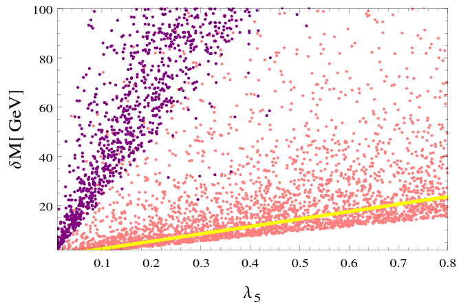
Figure 2 shows the variation of λ5\lambda_{5} and δ​M​(MH0−MA)\delta M(M_{H_{0}}-M_{A}) for different values of m22m_{22}. Purple, yellow and pink colours describe the variation for m22m_{22}=150, 2000 GeV and for 100−3000100-3000 GeV respectively. As the value of m22m_{22} is increasing it dominates the splitting effect of quartic couplings and the mass-splitting becomes lower and lower. Figure 2 depicts the mass splitting δ​M\delta M (MH0−MA)(M_{H_{0}}-M_{A}) with m22m_{22} for different values of λ5\lambda_{5}. Here the magenta and orange colours correspond to λ5=0.01,0.8\lambda_{5}=0.01,0.8 respectively and the cyan region corresponds to λ5=0.01−0.80\lambda_{5}=0.01-0.80. For lower values of m22m_{22}, mass splitting can be greater than ∼\sim 100 GeV and it comes down to ∼\sim 20 GeV for higher values m22∼3000m_{22}\sim 3000 GeV depending on the allowed parameter space.
Refer to caption
Refer to caption
Figure 2: 2: Variation of λ5\lambda_{5} verses δ​M​(MH0−MA)\delta M(M_{H_{0}}-M_{A}) in GeV for different values of m22m_{22}. Purple, yellow and pink colours describe the variation for m22m_{22}=150, 2000 GeV and for 100−3000100-3000 GeV respectively; 2: Variation of m22m_{22} verses δ​M​(MH0−MA)\delta M(M_{H_{0}}-M_{A}) in GeV for different values of λ5\lambda_{5}. Here the magenta and orange colours correspond to λ5=0.01,0.8\lambda_{5}=0.01,0.8 respectively and the cyan region corresponds to λ5=0.01−0.80\lambda_{5}=0.01-0.80. For lower values of m22m_{22}, mass splitting can be greater than ∼\sim 100 GeV and it comes down to ∼\sim 20 GeV for higher values m22∼3000m_{22}\sim 3000 GeV depending on the allowed parameter space.
Figure 3: Variation of MT±M_{T}^{\pm} vs MT0M_{T_{0}} in GeV. At the tree-level there is no mass-splitting and the width describes the different solutions allowed by parameter space.

Figure 3 describes the variation of MT±M_{T}^{\pm} vs MT0M_{T_{0}} in GeV at tree-level. We see that at the tree-level there is no mass-splitting between triplet states. One has to rely on the loop-contributions for 𝒪⁡(166)\mathcal{O}(166) MeV mass splitting between T±T^{\pm} and T0T_{0} which will be crucial for the phenomenological studies Cirelli:2005uq.

5 Perturbativity Bound

To emulate the theoretical bounds from perturbative unitarity of the dimensionless couplings, we impose that all dimensionless couplings of the model must remain perturbative for a given value of the energy scale μ\mu, i.e. the couplings must satisfy the following constraints:

|λi|≤ 4​π,|gj|≤ 4​π,|Yk|≤4​π,\displaystyle\left|\lambda_{i}\right|\ \leq\ 4\pi,\hskip 20.00003pt\left|g_{j}\right|\ \leq\ 4\pi,\hskip 20.00003pt\left|Y_{k}\right|\ \leq\ \sqrt{4\pi}\,, (12)

where λi\lambda_{i} with i=1,2,3,4,5i=1,2,3,4,5 are the scalar quartic couplings; gjg_{j} with j=1,2j=1,2 are EW gauge couplings;11 1 The running of the strong coupling g3g_{3} is same as in the SM, so we do not show it here. and YkY_{k} with k=u,d,ℓk=u,d,\ell are all Yukawa couplings for the up, down types quarks and leptons respectively. The two-loop beta functions generated by SARAH 4.13.0 Staub:2013tta, given in Appendix A and Appendix B are used to check the variations of the dimensionless couplings with the scale of the variation (μ\mu in GeV).

Figure 4: Two-loop running of the scalar quartic couplings λ3\lambda_{3}, λ4\lambda_{4} and λ5\lambda_{5} as a function of perturbative scale. Here red, green, blue and purple curves in each plot correspond to different initial conditions for λi\lambda_{i} (with i=2,3,4,5i=2,3,4,5) at the EW scale, representative of very weak (λi=0.01\lambda_{i}=0.01), weak (λi=0.1\lambda_{i}=0.1), moderate (λi=0.4\lambda_{i}=0.4) and strong (λi=0.8\lambda_{i}=0.8) coupling limits respectively.

The perturbativity behaviour of the scalar quartic couplings λ3,4,5\lambda_{3,4,5} is studied in Figure 4-4 respectively where the other quartic couplings λ(i=2,3,4,5)\lambda_{(i=2,3,4,5)} are fixed at some values. Here red, green, blue and purple curves in each plot correspond to different initial conditions for other λi\lambda_{i} at the EW scale, representative of very weak (λi=0.01\lambda_{i}=0.01), weak (λi=0.10\lambda_{i}=0.10), moderate (λi=0.40\lambda_{i}=0.40) and strong (λi=0.80\lambda_{i}=0.80) coupling limits respectively. The dashed black line corresponds to Planck scale (101910^{19} GeV). Higgs quartic coupling λ3\lambda_{3} remains perturbative till Planck scale for λ3≲0.51,0.32\lambda_{3}\lesssim 0.51,0.32 for λi​(EW)=0.01,0.10\lambda_{i}(\rm{EW})=0.01,0.10 respectively as shown in Figure 4. For λi​(EW)=0.40,0.80\lambda_{i}(\rm{EW})=0.40,0.80 theory becomes non-perturbative at much lower scale ∼\sim 108.9, 105.610^{8.9},\,10^{5.6} GeV respectively for almost all initial values of λ3\lambda_{3}.

Figure 4 shows similar behaviour for λ4\lambda_{4} and here for the choice of λi​(EW)=0.01,0.10\lambda_{i}(\rm{EW})=0.01,0.10 the perturbative limits remain valid till Planck scale for λ4≲0.60, 0.30\lambda_{4}\lesssim 0.60,\,0.30 respectively. For higher values of λi​(EW)\lambda_{i}(\rm{EW}) the perturbative bounds remain similar to Figure 4. Figure 4 depicts the behaviour for λ5\lambda_{5} for the chosen other λi​(EW)\lambda_{i}(\rm{EW}). Here for λi​(EW)=0.01,0.10\lambda_{i}(\rm{EW})=0.01,0.10 the perturbative limit till Planck scale is valid for λ5\lambda_{5} ≲0.28, 0.19\lesssim 0.28,\,0.19 respectively. In general when λi≃0.1−0.2\lambda_{i}\simeq 0.1-0.2 at the EW scale, all the quartic couplings remains perturbative till Planck scale for IDM.

Figure 5: Two-loop running of the scalar quartic coupling λh​t\lambda_{ht} as a function of perturbative scale. Here red, green, blue and purple curves in each plot correspond to different initial conditions for λt\lambda_{t} and λh​t\lambda_{ht} at the EW scale, representative of very weak (λt=0.01\lambda_{t}=0.01), weak (λt=0.1\lambda_{t}=0.1), moderate (λt=0.4\lambda_{t}=0.4) and strong (λt=0.8\lambda_{t}=0.8) coupling limits respectively.

Figure 5 shows the variation of quartic coupling λh​t\lambda_{ht} which describes the interaction between SM doublet and Y=0Y=0 Higgs triplet. The dashed black line corresponds to the Planck scale. Due to the existence of lesser number of quartic couplings compared to the 2HDM, the theory stays perturbative till Planck scale for much higher values of quartic couplings λt,λh​t\lambda_{t},\lambda_{ht}. For choice of λt​(EW)\lambda_{t}(\rm EW)=0.01, 0.1, 0.4 and 0.8 the perturbative limits remains valid till Planck scale for λh​t=0.1−0.8\lambda_{ht}=0.1-0.8 at EW scale. Perturbativity puts upper bound on Higgs quartic coupling λh​t≲0.50\lambda_{ht}\lesssim 0.50 for λt=1.3\lambda_{t}=1.3 at the EW scale. For ITM case the SM-like Higgs quartic coupling only takes part in the EWSB breaking and its values at two-loop level is fixed at 0.12640.1264 for the SM-like Higgs boson mass at 125.50125.50 GeV.

6 Stability Bound

In this section we discuss the stability of Higgs potential via two different approaches. Firstly via calculating two-loop scalar quartic couplings and checking if the SM-like Higgs quartic coupling λh\lambda_{h} is getting negative at some scale. In this case λh=λ1\lambda_{h}=\lambda_{1} at tree-level but at one-loop and two-loop levels λh\lambda_{h} gets contribution from SM fields as well as the BSM scalars as we describe in the subsection 6.1. For the simplicity in subsection 6.1 we give the expressions of the corresponding beta functions at one-loop level and in the Appendix A, B the two-loop beta functions are given.

6.1 RG Evolution of the Scalar Quartic Couplings

To study the evaluations of dimensionless couplings we implemented both the IDM and the ITM scenarios in SARAH 4.13.0 Staub:2013tta and the corresponding β\beta-functions for various gauge, quartic and Yukawa couplings are calculated at one- and two-loop levels. The explicit expressions for the two-loop β\beta-functions can be found in Appendix A, B and they are used in our numerical analysis of vacuum stability in this section. To illustrate the effect of the Yukawa and additional scalar quartic couplings on the RG evolution of the SM-like Higgs quartic coupling λ1\lambda_{1} in the scalar potential (1) and (8), let us first look at the one-loop β\beta-functions. λh=λ1\lambda_{h}=\lambda_{1} at tree-level and at the one-loop level, the β\beta-function for the SM Higgs quartic coupling in this model receives two different contributions: one from the SM gauge, Yukawa, quartic interactions and the second from the inert scalar sectors of IDM/ITM as shown below:

βλ1=βλ1SM+βλ1IDM/ITM,\beta_{\lambda_{1}}=\beta_{\lambda_{1}}^{\rm SM}+\beta_{\lambda_{1}}^{\rm IDM/ITM}, (13)

where,

βλ1SM\displaystyle\beta_{\lambda_{1}}^{\rm SM} =\displaystyle= 116​π2[27200g14+920g12g22+98g24−95g12λ1−9g22λ1+24λ12\displaystyle\frac{1}{16\pi^{2}}\Bigg[\frac{27}{200}g_{1}^{4}+\frac{9}{20}g_{1}^{2}g_{2}^{2}+\frac{9}{8}g_{2}^{4}-\frac{9}{5}g_{1}^{2}\lambda_{1}-9g_{2}^{2}\lambda_{1}+24\lambda_{1}^{2} (14)
+12​λ1​Tr​(Yu​Yu†)+12​λ1​Tr​(Yd​Yd†)+4​λ1​Tr​(Ye​Ye†)\displaystyle+12\lambda_{1}\mbox{Tr}\Big({Y_{u}Y_{u}^{\dagger}}\Big)+12\lambda_{1}{\rm Tr}\Big({Y_{d}Y_{d}^{\dagger}}\Big)+4\lambda_{1}\mbox{Tr}\Big({Y_{e}Y_{e}^{\dagger}}\Big)
−6Tr(YuYu†YuYu†)−6Tr(YdYd†YdYd†)−2Tr(YℓYℓ†YℓYℓ†)],\displaystyle-6\mbox{Tr}\Big({Y_{u}Y_{u}^{\dagger}Y_{u}Y_{u}^{\dagger}}\Big)-6\mbox{Tr}\Big({Y_{d}Y_{d}^{\dagger}Y_{d}Y_{d}^{\dagger}}\Big)-2\mbox{Tr}\Big({Y_{\ell}Y_{\ell}^{\dagger}Y_{\ell}Y_{\ell}^{\dagger}}\Big)\Bigg],
βλ1IDM\displaystyle\beta_{\lambda_{1}}^{\rm IDM} =\displaystyle= 116​π2​[2​λ32+2​λ3​λ4+λ42+4​λ52].\displaystyle\frac{1}{16\pi^{2}}\Big[2\lambda_{3}^{2}+2\lambda_{3}\lambda_{4}+\lambda_{4}^{2}+4\lambda_{5}^{2}\Big]. (15)
βλ1ITM\displaystyle\beta_{\lambda_{1}}^{\rm ITM} =\displaystyle= 116​π2​[8​λh​t2].\displaystyle\frac{1}{16\pi^{2}}\Big[8\lambda_{ht}^{2}\Big]. (16)

Here g1,g2,g3g_{1},g_{2},g_{3} are respectively the U​(1)YU(1)_{Y}, S​U​(2)LSU(2)_{L} and S​U​(3)cSU(3)_{c} gauge couplings, and Yu,Yd,YℓY_{u},Y_{d},Y_{\ell} are respectively the up, down and lepton-Yukawa coupling matrices of SM. We use the SM input values for these parameters at the EW scale: λ1=0.1264\lambda_{1}=0.1264, g1=0.3583g_{1}=0.3583, g2=0.6478g_{2}=0.6478, yt=0.9369y_{t}=0.9369 and other Yukawa couplings are neglected Degrassi:2012ry; Buttazzo:2013uya.

Figure 6: Two loop running of the SM like Higgs quartic coupling in IDM and ITM for four benchmark values of the Higgs quartic couplings (λ1=2,3,4,5)(\lambda_{1=2,3,4,5}) in IDM and (λh​t,t)(\lambda_{ht,t}) in ITM to be 0.010, 0.060, 0.068 and 0.100 respectively. Here the red curve corresponds to the inert 2HDM and the green curve corresponds to the inert triplet Model.

Figure 6 depicts the running of SM-like Higgs quartic coupling at two-loop level for four benchmark points with (λ2,3,4,5)(\lambda_{2,3,4,5}) for IDM and (λh​t,t)(\lambda_{ht,t}) for ITM to be 0.010, 0.060, 0.068 and 0.100 respectively. For both the cases λ1=0.1264\lambda_{1}=0.1264 is kept at two-loop level for the SM-like Higgs boson mass at 125.5125.5 GeV. Here the red curve corresponds to the IDM and the green curve corresponds to the ITM. For λi​(EW)\lambda_{i}\rm(EW)=0.010, in Figure 6, the effect of scalars on stability is less and both IDM and ITM becomes unstable at same scale ∼109.7\sim 10^{9.7}. In Figure 6 for λi​(EW)=0.060\lambda_{i}(\rm{EW})=0.060 we see that the λh\lambda_{h} becomes negative around 101210^{12} GeV but λh\lambda_{h} turns upward at 101610^{16} GeV and touches zero value for 102010^{20} GeV in the case of IDM while for ITM it still stays negative. As λi​(EW)\lambda_{i}(\rm{EW}) enhances to 0.068 in Figure 6, the stability scale increases to ∼1013.5\sim 10^{13.5} in ITM while IDM becomes completely stable. Since, there are more number of scalars in IDM than ITM, the theory becomes stable at much lower values of λi\lambda_{i}. Further enhancement of λi​(E​W)\lambda_{i}(EW) to 0.100, Figure 6 makes both IDM and ITM stable till Planck scale.

6.2 Vacuum Stability from RG-improved potential Approach

In this section, we investigate the vacuum stability via RG-improved effective potential approach by Coleman and Weinberg Coleman:1973jx, and calculate the effective potential at one-loop for IDM/ITM. The parameter space of the models are then scanned for the stability, metastability and instability of the potential by calculating the effective Higgs quartic coupling and implementing the constraints as discussed in the paragraph follows.

Before going to quantum corrected potential lets look at the stability conditions of the tree-level potential of IDM/ITM. The tree-level potential of IDM is given in Eq. (1) and the potential is bounded from below in all the directions is ensured by the tree-level stability conditions given by Branco:2011iw

λ1≥ 0,λ2≥ 0,λ3≥−λ1​λ2,λ3+λ4−|λ5|≥−λ1​λ2.\displaystyle\lambda_{1}\ \geq\ 0\,,\hskip 10.00002pt\lambda_{2}\ \geq\ 0\,,\hskip 10.00002pt\lambda_{3}\ \geq\ -\sqrt{\lambda_{1}\lambda_{2}}\,,\hskip 10.00002pt\lambda_{3}+\lambda_{4}-|\lambda_{5}|\ \geq\ -\sqrt{\lambda_{1}\lambda_{2}}\,. (17)

Similarly, the tree-level potential of ITM is given in Eq. (8) and the corresponding tree-level stability conditions are given by Araki:2010zz

λh≥ 0,λt≥ 0,|λh​t|≥−2​λh​λt.\displaystyle\lambda_{h}\ \geq\ 0\,,\hskip 10.00002pt\lambda_{t}\ \geq\ 0\,,\hskip 10.00002pt|\lambda_{ht}|\geq-2\sqrt{\lambda_{h}\lambda_{t}}. (18)

Considering the running of couplings with the energy scale in the SM, we know that the Higgs quartic coupling λh\lambda_{h} gets a negative contribution from top Yukawa coupling yty_{t}, which makes it negative around 109−1010^{9-10} GeV Buttazzo:2013uya; EliasMiro:2011aa and we expect a second deeper minimum for the high field values. Since, the other minimum exists at much higher scale than the EW minimum, we can safely consider the effective potential in the hh-direction to be

Veff​(h,μ)≃λeff​(h,μ)​h44,with​h≫v,\displaystyle V_{\rm eff}(h,\mu)\ \simeq\ \lambda_{\rm eff}(h,\mu)\frac{h^{4}}{4},\hskip 10.00002pt{\rm with}\penalty\ h\gg v\,, (19)

where λeff​(h,μ)\lambda_{\rm eff}(h,\mu) is the effective quartic coupling which can be calculated from the RG-improved potential. The stability of the vacuum can then be guaranteed at a given scale μ\mu by demanding that λeff​(h,μ)≥0\lambda_{\rm eff}(h,\mu)\geq 0. We follow the same strategy as in the SM in order to calculate λeff​(h,μ)\lambda_{\rm eff}(h,\mu) in our model, as described below.

The one-loop RG-improved effective potential in our model can be written as

Veff=V0+V1SM+V1IDM/ITM,\displaystyle V_{\rm eff}\ =\ V_{0}+V_{1}^{\rm SM}+V_{1}^{\rm IDM/ITM}\,, (20)

where V0V_{0} is the tree-level potential given by Eq. (1) for IDM and Eq. (8) for ITM. V1SMV_{1}^{\rm SM} is the effective Coleman-Weinberg potential of the SM that contains all the one-loop corrections involving the SM particles at zero temperature with vanishing momenta. V1IDMV_{1}^{\rm IDM} and V1ITMV_{1}^{\rm ITM} are the corresponding one-loop effective potential terms from the IDM and the ITM loops. In general, V1V_{1} can be written as

V1​(h,μ)=164​π2​∑i(−1)F​ni​Mi4​(h)​[log⁡Mi2​(h)μ2−ci],\displaystyle V_{1}(h,\mu)\ =\ \frac{1}{64\pi^{2}}\sum_{i}(-1)^{F}n_{i}M_{i}^{4}(h)\Bigg[\log\frac{M_{i}^{2}(h)}{\mu^{2}}-c_{i}\Bigg], (21)

where the sum runs over all the particles that couple to the hh-field, F=1​and​ 0F=1\,\rm{and}\,0 for fermions and the bosons in the loop, nin_{i} is the number of degrees of freedom of each particle, Mi2M_{i}^{2} are the tree-level field-dependent masses given by

Mi2​(h)=κi​h2−κi′,\displaystyle M_{i}^{2}(h)\ =\ \kappa_{i}h^{2}-\kappa^{\prime}_{i}, (22)

with the coefficients given in Table 1 and m2m^{2} corresponds to Higgs mass parameter. Note that the massless particles do not contribute to Eq. (22), and so to Eq. (21). Therefore, for the SM fermions, we only include the dominant contribution from top quarks, and neglect the other quarks. We take h=μh=\mu for the numerical analysis as at that scale the potential remains scale invariant Casas:1994us.

Particles ii FF nin_{i} cic_{i} κi\kappa_{i} κi′\kappa^{\prime}_{i}
W±W^{\pm} 0 6 5/6 g22/4g_{2}^{2}/4 0
ZZ 0 3 5/6 (g12+g22)/4(g_{1}^{2}+g_{2}^{2})/4 0
SM tt 1 12 3/2 Yt2Y_{t}^{2} 0
hh 0 1 3/2 λh\lambda_{h} m2m^{2}
G±G^{\pm} 0 2 3/2 λh\lambda_{h} m2m^{2}
G0G^{0} 0 1 3/2 λh\lambda_{h} m2m^{2}
H±H^{\pm} 0 2 3/2 λ3/2\lambda_{3}/2 0
IDM HH 0 1 3/2 (λ3+λ4+2​λ5)/2(\lambda_{3}+\lambda_{4}+2\lambda_{5})/2 0
AA 0 1 3/2 (λ3+λ4−2​λ5)/2(\lambda_{3}+\lambda_{4}-2\lambda_{5})/2 0
ITM T±T^{\pm} 0 2 3/2 λh​t/2\lambda_{ht}/2 0
TT 0 1 3/2 λh​t/2\lambda_{ht}/2 0
Table 1: Coefficients entering in the Coleman-Weinberg effective potential, cf. Eq. (21).

Using Eq. (21) for the one-loop potentials, the full effective potential in Eq. (20) can be written in terms of an effective quartic coupling as in Eq. (19). This effective coupling can be written as follows:

λeff​(h,μ)\displaystyle\lambda_{\rm eff}\left(h,\mu\right) ≃λh​(μ)⏟tree-level+116​π2​∑i=W±,Z,t,h,G±,G0ni​κi2​[log⁡κi​h2μ2−ci]⏟Contribution from SM+116​π2​∑i=H,A,H±ni​κi2​[log⁡κi​h2μ2−ci]⏟ Contribution from IDM/ITM ,\displaystyle\ \simeq\ \underbrace{\lambda_{h}\left(\mu\right)}_{\text{tree-level}}+\underbrace{\frac{1}{16\pi^{2}}\sum_{\begin{subarray}{c}i=W^{\pm},Z,t,\\ h,G^{\pm},G^{0}\end{subarray}}n_{i}\kappa_{i}^{2}\Big[\log\frac{\kappa_{i}h^{2}}{\mu^{2}}-c_{i}\Big]}_{\text{Contribution from SM}}+\underbrace{\frac{1}{16\pi^{2}}\sum_{i=H,A,H^{\pm}}n_{i}\kappa_{i}^{2}\Big[\log\frac{\kappa_{i}h^{2}}{\mu^{2}}-c_{i}\Big]}_{\text{ Contribution from IDM/ITM }}, (23)

where the corresponding coefficients for all the required fields are given in the Table 1. The nature of λeff\lambda_{\rm eff} in the models thus guides us to identify the possible instability and metastability regions, as discussed below.

6.3 Stable, Metastable and Unstable Regions

The parameter space where λeff>0\lambda_{\rm eff}>0 is termed as the stable region, since the EW vacuum is the global minimum in this region. For λeff<0\lambda_{\rm eff}<0, there exists a second minimum deeper than the EW vacuum. In this case, the EW vacuum could be either unstable or metastable, depending on the tunnelling probability from the EW vacuum to the true vacuum. The parameter space with λeff<0\lambda_{\rm eff}<0, but with the tunnelling lifetime longer than the age of the universe is termed as the metastable region. The expression for the tunnelling probability to the deeper vacuum at zero temperature is given by

P=T04​μ4​e−8​π23​λeff​(μ),\rm P\ =\rm\ T_{0}^{4}{\mu}^{4}e^{\frac{-8{\pi}^{2}}{3\lambda_{\rm eff}(\mu)}}\,, (24)

where T0T_{0} is the age of the universe and μ\mu denotes the scale where the probability is maximized, i.e. ∂P∂μ=0\frac{\partial P}{\partial\mu}=0. This gives us a relation between the λ\lambda values at different scales:

λeff​(μ)=λeff​(v)1−32​π2​log⁡(vμ)​λeff​(v),\displaystyle\lambda_{\rm eff}(\mu)\ =\ \frac{\lambda_{\rm eff}(v)}{1-\frac{3}{2\pi^{2}}\log\left(\frac{v}{\mu}\right)\lambda_{\rm eff}(v)}\,, (25)

where v≃246v\simeq 246 GeV is the EW VEV. Setting P=1P=1, T=1010T=10^{10} years and μ=v\mu=v in Eq. (24), we find λeff​(v)\lambda_{\rm eff}(v) =0.0623. The condition P<1P<1, for a universe about T=1010T=10^{10} years old is equivalent to the requirement that the tunnelling lifetime from the EW vacuum to the deeper one is larger than T0T_{0} and we obtain the following condition for metastability Isidori:2001bm:

0>λeff​(μ)≳−0.0651−0.01​log⁡(vμ).\displaystyle 0\ >\ \lambda_{\rm eff}(\mu)\ \gtrsim\ \frac{-0.065}{1-0.01\log\left(\frac{v}{\mu}\right)}. (26)

The remaining parameter space with λeff<0\lambda_{\rm eff}<0, where the condition (26) is not satisfied is termed as the unstable region. As can be seen from Eq. (23), these regions depend on the energy scale μ\mu, as well as the model parameters, including the gauge, scalar quartic and Yukawa couplings.

Figure 7: Phase diagram in terms of Higgs and top pole masses in GeV for 7: SM like scenario, 7: Inert Higgs Doublet Model and 7: Inert Higgs Triplet Model. The red colour corresponds to the unstable region, yellow color corresponds to the metastable region and the green colour corresponds to the stable region. The contours and the dot show the current experimental 1​σ,2​σ,3​σ1\sigma,2\sigma,3\sigma regions and central value in the (Mh,Mt)(M_{h},M_{t}) plane.

Figure 7 represents the phase diagram in terms of Higgs and top pole masses in GeV. The red, yellow and green regions correspond to the unstable, metastable and stable regions respectively. The contours and the dot show the current experimental 1​σ,2​σ,3​σ1\sigma,2\sigma,3\sigma regions and central value in the (Mh,Mt)(M_{h},M_{t}) plane Buttazzo:2013uya; Masina:2012tz. To obtain the regions we vary all the λi​(EW)=0.01−0.80\lambda_{i}(\rm EW)=0.01-0.80 for random values maintaining the Planck scale perturbativity and also maintain the mhm_{h} and mtm_{t} within limits shown in Figure 7. Figure 7 shows the scenario where λ1≠0\lambda_{1}\neq 0 and all other λi=0\lambda_{i}=0 and clearly the region is in metastbale state as expected for SM Buttazzo:2013uya. Introduction of inert doublet adds more scalars to the effective potential so the λeff\lambda_{\rm{eff}} becomes more positive and the region is fully in the stable region as can be seen from Figure 7. In Figure 7 we depicts the scenario for ITM, where such extra scalar degrees of freedoms are lesser than IDM but more than SM, so the 3​σ3\sigma contour in mh−mtm_{h}-m_{t} plane includes some region of metastability. In this context we also want to mention that the extra scalars are necessary and come as saviour for the models with right-handed neutrino with 𝒪⁡(1)\mathcal{O}(1) neutrino Yukawa coupling exwfermion-Garg:2017iva.

7 Calculation of Relic Density in freeze out scenario for IDM and ITM

After the theoretical constraints from perturbativity and vacuum stability we focus on the constraints coming from the dark sector. In case of IDM lightest of the AA and H0H_{0} can be dark matter candidate being Z2Z_{2}-odd. For our study we focus on the parameter space for which AA is the lightest and serves as the DM. However, for the ITM case we have only one Z2Z_{2}-odd neutral scalar, i.e. T0T_{0} which serves as the DM. The different possible annihilation and co-annihilation diagrams are shown in Figure 8 for IDM and in Figure 9 for ITM respectively. Both of these DM candidates A/T0A/T_{0} are charged under S​U​(2)SU(2) and thus the dominant mode of annihilation is W±​W∓W^{\pm}W^{\mp}. Being Y=0Y=0 triplet in the case of ITM there is no direct annihilation to Z​ZZZ via contact or tt-channel, which exist in the case of IDM. However, a ss-channel annihilation via SM Higgs boson is possible. Apart from the annihilation channels, T±​T0T^{\pm}T_{0} and H±​AH^{\pm}A co-annihilation to W±​Z/γW^{\pm}Z/\gamma channels exist in both the scenarios which are secondary contributors. In both the cases DM annihilation channels to h​hhh is subdominant one and annihilation to fermion pair is negligible.

The matrix element squared for the dominant DM annihilation and co-annihilation channels, i.e. to W±​W∓,Z​ZW^{\pm}W^{\mp},\,ZZ and Z​W±ZW^{\pm} are given in the Appendix C. Once we have the matrix element squared we calculate the ⟨σ​v⟩\big<\sigma v\big> in the non-relativistic limit following Eq. 27

⟨σ​v⟩=1kf!​16​π​s​s−4​mf2mi​|ℳ|2¯\big<\sigma v\big>=\frac{1}{k_{f}!16\pi s}\frac{\sqrt{s-4m^{2}_{f}}}{m_{i}}{\overline{|\mathcal{M}|^{2}}} (27)

where s=Ec​m2s=E^{2}_{cm}, vv stands for the relative velocity of the dark matter particles and kfk_{f} is the symmetry factor for the identical particles in the final states. |ℳ|2¯\overline{|\mathcal{M}|^{2}} is the spin averaged matrix element squared for annihilation and co-annhilation channels. For the numerical calculation we have taken all possible interference terms involved in the matrix element square calculation which are not shown in the Appendix C.

Equipped with the ⟨σ​v⟩\big<\sigma v\big> for different annihilation modes we now examine the thermal relic abundance of DM particle. ϕDM\phi_{\rm{DM}} (A/T0A/T_{0} for IDM/ITM) via Freeze-out mechanism Banerjee:2019luv; freezeout. The evolution of the number density of DM is obtained by solving the Boltzmann equation Araki:2011hm

d​nϕDMd​t+3HnϕDM=−⟨σv⟩(nϕDM2−nϕDM,e​q2),\frac{dn_{\phi_{\rm{DM}}}}{dt}+3Hn_{\phi_{\rm{DM}}}=-\big<\sigma v\big>(n^{2}_{\phi_{\rm{DM}}}-n^{2}_{\phi_{\rm{DM}},eq}), (28)

where H is the Hubble parameter, nϕDMn_{\phi_{\rm{DM}}}, nϕDM,e​qn_{\phi_{\rm{DM}},eq} and σ\sigma are the number density of DM particle, the number density in thermal equilibrium and the total annihilation cross-section of ϕDM\phi_{\rm{DM}} respectively. All the particles in the Z2Z_{2}-odd multiplets for both IDM/ITM will eventually contribute with ⟨σ​v⟩\big<\sigma v\big>. Before the onset of freeze-out, the universe was hot and dense and as the universe expands, the temperature falls down. In this scenario the respective dark matter particles will not be able to find each other fast enough to maintain the equilibrium abundance. So when the equilibrium ends and the freeze-out starts, inert particles T0T_{0} and AA, can contribute in the relic density of DM through freeze-out mechanism freezeout. Freeze-out of ϕD​M\phi_{DM} determines the DM relic abundance in today’s time which gets constraints from the WMAP and Planck experiments Planck with the current value

ΩDM​h2=0.1199±0.0027,\displaystyle\rm\Omega_{DM}h^{2}=0.1199\pm 0.0027, (29)

where h=0.67±0.012\rm h=0.67\pm 0.012 is the scaled current Hubble parameter in units of 100​k​m/s.Mpc\rm 100km/s.Mpc. Here, we use this value as upper bound on the contribution on dark matter production for the models IDM Banerjee:2019luv and ITM Tripletex.

Refer to caption
Figure 8: Dominant annihilation and co-annihilation modes that contribute to DM relic for IDM.
Refer to caption
Figure 9: Dominant annihilation and co-annihilation modes that contribute to DM relic for ITM.

Unlike IDM, the mass splitting between dark matter (T0)(T_{0}) and charged components (T±)(T^{\pm}) is much smaller for ITM, 𝒪⁡(166)\mathcal{O}(166) MeV. Thus the co-annihilation T0​T±→Z​W±T_{0}T^{\pm}\rightarrow ZW^{\pm} contribution is larger as compared to IDM. Below we scan the parameter space for both IDM and ITM to find out the regions with correct DM relic as given in Eq. (29).

For this scan we take the allowed parameter space from perturbativity and stability till Planck scale for the analysis of correct DM relic density by Micromegas 5.0.8 Belanger:2008sj; Belanger:2006is; Belanger:2010pz. There we have taken contributions from all possible annhilation and co-annihilation channels and the interference effects therein. Figure 10 describes the variation of relic density with the masses of charged Higgs boson and DM (A/T0A/T_{0} for IDM/ITM). The colour code of DM relic (Ω​h2\Omega h^{2}) is shown from blue to red for 0.0−0.40.0-0.4 for both IDM and ITM respectively. The correct values of Ω​h2=0.1199±0.0027\Omega h^{2}=0.1199\pm 0.0027 is specified by a star in both the cases. We can read from Figure 10 that for IDM MA>⁣∼700M_{A}\mathrel{\mathop{\kern 0.0pt\hbox to0.0pt{\raise 0.86108pt\hbox{$>$}\hss}}\lower 3.87495pt\hbox{\kern-1.90002pt$\sim$}}700 GeV corresponds to correct DM relic value. However, for ITM the correct relic value corresponds to MT0>⁣∼1176M_{T_{0}}\mathrel{\mathop{\kern 0.0pt\hbox to0.0pt{\raise 0.86108pt\hbox{$>$}\hss}}\lower 3.87495pt\hbox{\kern-1.90002pt$\sim$}}1176 GeV as shown in Figure 10. The presence of one extra Z2Z_{2}-odd scalar in IDM compared to ITM, results into higher the DM number density in IDM case and thus requires more annihilation or co-annihilation modes to obtain the correct relic compared to the ITM case, leading to lower mass bound on DM mass for IDM. Even for relatively heavier mass spectrum of IDM corresponds mass gap of the order of 𝒪⁡(1)\mathcal{O}(1) GeV among the Z2Z_{2}-odd particles. In comparison the ITM scenario leads to even smaller mass gap 𝒪⁡(166)\mathcal{O}(166) MeV coming from one-loop corrections, which leads to a dominant co-annihilation processes obtaining the correct relic as pointed out earlier.

Refer to caption
Refer to caption
Figure 10: 3D plot describing the variation of relic density with dark matter mass and charged Higgs boson mass in GeV. 10: IDM, 10: ITM. The correct relic density corresponds to DM mass >⁣∼700\mathrel{\mathop{\kern 0.0pt\hbox to0.0pt{\raise 0.86108pt\hbox{$>$}\hss}}\lower 3.87495pt\hbox{\kern-1.90002pt$\sim$}}700 GeV in IDM and the mass splitting between DM mass and charged Higgs boson mass is order of 𝒪⁡(1)\mathcal{O}(1) GeV. In ITM scenario corresponds to DM mass of >⁣∼1176\mathrel{\mathop{\kern 0.0pt\hbox to0.0pt{\raise 0.86108pt\hbox{$>$}\hss}}\lower 3.87495pt\hbox{\kern-1.90002pt$\sim$}}1176 GeV with the mass gap being 𝒪⁡(166)\mathcal{O}(166) MeV at one-loop.

8 Constrains from Direct Dark Matter experiments

In this section, we discuss the direct detection prospects of DM candidate for both IDM and ITM scenarios. Dark matter can be detected via elastic scattering with terrestrial detectors, the so-called direct detection method. From the particle physics point of view, the quantity that determines the direct detection rate is the dark matter-nucleon (DM−N\rm{DM}-N) scattering cross-section. In the IDM, the DM−N\rm{DM}-N scattering process relevant for direct detection is Higgs-mediated. The tree-level spin-independent DM-nucleon interaction cross section, in IDM scenario Diaz:2015pyv; Garcia-Cely:2015ysa is given by Eq. (30)

σSI=λ3452​fN24​π​Mh4​MN4(MN+MA)2,\rm\sigma_{SI}=\frac{\lambda_{345}^{2}f_{N}^{2}}{4\pi M_{h}^{4}}\frac{M_{N}^{4}}{(M_{N}+M_{A})^{2}}, (30)

were MhM_{h} is the mass of the SM-like Higgs boson, MA\rm M_{A} is the mass of the DM candidate, MNM_{N} is the nucleon mass that we took equal to the average of proton and neutron masses, fNf_{N} is the nucleon form factor, taken equal to 0.3 for the subsequent analysis and λ345=λ3+λ4−2​λ5\lambda_{345}=\lambda_{3}+\lambda_{4}-2\lambda_{5} with λ5>0\lambda_{5}>0, is the combined coupling that is responsible for the scattering. we have used Micromegas 5.0.8 Belanger:2008sj; Belanger:2006is; Belanger:2010pz to calculate the direct spin-independent scattering cross-sections and DM relic density for the parameter space and later compare with the experimental bounds from different direct detection experiments as discussed later.

In the case of ITM, the T0T_{0} DM candidate can interact with nucleon by exchanging Higgs boson and the DM-nucleon scattering cross section is given by Tripletex Eq 31

σSI=λht2​fN24​π​Mh4​MN4(MN+MT0)2,\rm\sigma_{SI}=\frac{\lambda_{ht}^{2}f_{N}^{2}}{4\pi M_{h}^{4}}\frac{M_{N}^{4}}{(M_{N}+M_{T_{0}})^{2}}, (31)

where the coupling constant fNf_{N} is given by nuclear matrix elements and MN=0.939\rm M_{N}=0.939 GeV is nucleon mass which is average of the proton and neutron masses, MhM_{h} is the SM-like Higgs boson mass, MT0M_{T_{0}} is the dark matter mass and λh​t\lambda_{ht} is only responsible Higgs coupling here.

There are several experiments to detect DM particles directly through the elastic DM-nucleon scattering. The strong bounds on the DM-nucleon cross section are obtained from XENON100 Aprile:2012nq, LUX Akerib:2013tjd and XENON1T Aprile:2015uzo experiments. The minimum upper limits on the spin independent cross sections are:

XENON100:σSI≤2.0×10−45​cm2\displaystyle\rm XENON100:\rm\sigma_{SI}\leq 2.0\times 10^{-45}\,cm^{2} (32)
LUX:σSI≤7.6×10−46​cm2\displaystyle\ \rm LUX:\rm\sigma_{SI}\leq 7.6\times 10^{-46}\,cm^{2}\, (33)
XENON1T:σSI≤1.6×10−47​cm2\displaystyle\rm XENON1T:\rm\sigma_{SI}\leq 1.6\times 10^{-47}\,cm^{2}\, (34)
XENONnT:σSI≤1.6×10−48​cm2.\displaystyle\rm XENONnT:\rm\sigma_{SI}\leq 1.6\times 10^{-48}\,cm^{2}. (35)

Figure 11 describes the variation of spin independent (SI)\rm(SI) DM-nucleon scattering cross-section with DM mass for both IDM and ITM. The red colour corresponds to the cross-section bound satisfied by XENON100 experiment Aprile:2012nq, green colour satisfies the LUX experimental bound Akerib:2013tjd and the blue colour corresponds to the experimental bound of XENON1T experiment Aprile:2015uzo for both IDM and ITM. The cross-section varies with the DM mass and the Higgs quartic coupling λ345\lambda_{345} for IDM and λh​t\lambda_{ht} for ITM. If the Higgs quartic coupling is chosen to be small enough λ345=0.01\lambda_{345}=0.01 for IDM, the minimum DM mass satisfying the XENON1T bound is 420420 GeV 11. Unfortunately this value of quartic coupling in ITM i.e. λh​t\lambda_{ht}=0.01 is not allowed by the vacuum stability. The enhancement in Higgs quartic coupling λ345/h​t=0.2\lambda_{345/ht}=0.2 increases the lower bound of DM mass to 27702770 GeV by XENON1T data11.

Figure 11: SI cross-section verses dark matter mass in GeV. Here we have shown XENON100, LUX and XENON1T data in red, green and blue regions respectively. Widths in green and blue regions are to make them transparent such that other bounds are visible.

The variation of DM mass with Higgs quartic coupling λ3\lambda_{3} in IDM and λh​t\lambda_{ht} in ITM is depicted in Figure 12. The light purple and blue colour describe the allowed regions by stability and perturbativity till Planck scale for IDM and ITM respectively. The black vertical lines correspond to the relic density bound satisfied by DM mass 700,1200700,1200 GeV for IDM, ITM respectively. The green and red colour points describe the minimum values of MDMM_{\rm{DM}} for a given λ345/λh​t\lambda_{345}/\lambda_{ht} for IDM and ITM respectively that satisfy the direct Dark matter constraint of XENON1T Aprile:2015uzo. In IDM the effective quartic coupling λ345\lambda_{345} allows to choose maximum allowed value of λ3\lambda_{3} satisfying the direct DM constraints, while in the case of ITM the minimum value of MDMM_{\rm{DM}} increases with increase in λh​t\lambda_{ht}.

Figure 12: Variation of DM mass with Higgs quartic coupling λ3\lambda_{3} in IDM and ITM. The light purple and blue color describe the allowed region by stability and perturbativity for IDM and ITM respectively. The black vertical lines correspond to the relic density bound satisfied by DM mass 700,1200700,1200 GeV for IDM, ITM respectively. The green and red coloured points describe the minimum value of MDMM_{\rm{DM}} for a given λ345/λh​t\lambda_{345}/\lambda_{ht} for IDM and ITM respectively that satisfy the direct Dark matter constraint of XENON1T.
Figure 13: Physical mass eigenstates of the Higgs bosons in IDM and ITM corresponding to lightest possible DM mass satisfying the correct DM relic. hh is the 125.5125.5 GeV SM-like Higgs boson. Green colour corresponds to physical mass eigenstates in IDM. where AA is DM with MA=700.18M_{A}=700.18 GeV and MH±=702.364M_{H}^{\pm}=702.364 GeV, MH0=708.314M_{H_{0}}=708.314 GeV respectively. For ITM the lightest possible DM mass is MT0=1176.00M_{T_{0}}=1176.00 GeV along with almost degenrate charged Higgs mass MT±=1176.16M_{T^{\pm}}=1176.16 GeV represented in blue colour.

Figure 13 describes the mass spectrum for both IDM and ITM allowed by perturbativity and vacuum stability till Planck scale, DM relic density and DM-nucleon scattering cross-section. The lightest allowed values for IDM in the case are: MA=700.18M_{A}=700.18 GeV, MH±=702.36M_{H}^{\pm}=702.36 GeV, MH0=708.31M_{H_{0}}=708.31 GeV. The same reveals the lightest values for ITM are MT​0=1176.00M_{T0}=1176.00 GeV and MT±=1176.16M_{T^{\pm}}=1176.16 GeV where as the SM-like Higgs stays with mass 125.5 GeV for both the cases. One more number of Z2Z_{2}-odd field in IDM as compared to ITM which contributes to the number density of the dark matter. Thus IDM requires more annihilation cross-sections than ITM in getting the correct DM relic, which results in lower DM mass (∼700\sim 700) GeV for IDM as compared to ∼1.2\sim 1.2 TeV for ITM.

9 Constraints from H.E.S.S. and Fermi-Lat experiemtns

Indirect detection of dark matter is an interesting way to probe particle dark matter models. Among the few targets are Galactic centre and Dwarf Spheroidal Galaxies (dSphs), where dark matter annihilate or semi-annihilate into electron, positron, neutrinos, etc., yield gamma rays of different energies which are then observed by various telescopes. If the gamma-ray observation from different galactic sources are used as standard candles then any excess on the measured gamma-ray spectra can be used to probe the dark matter annihilation or co-annihilation channels.

The expected gamma-ray flux coming from the dark matter annihilation for DM​DM→SM​SM\rm DM\,DM\to SM\,SM can be written as

d​ϕγd​E=18​π​mD​M2<σ​v>d​Nγd​E​J,\frac{d\phi_{\gamma}}{dE}=\frac{1}{8\pi m^{2}_{DM}}<\sigma v>\frac{dN_{\gamma}}{dE}J, (36)

where mD​Mm_{DM} is the DM mass; which is mA​(mT0)m_{A}(m_{T_{0}}) for IDM (ITM), <σ​v><\sigma v> is the annihilation cross-section, d​Nγd​E\frac{dN_{\gamma}}{dE} is the gamma-ray spectrum and JJ is the JJ-factor which takes into account all the astrophysical processes and is given by,

J=∫r.o.id​Ω​∫l.o.sρDM2​𝑑l,J=\int_{r.o.i}d\Omega\int_{l.o.s}\rho^{2}_{\rm DM}dl, (37)

where ρDM2\rho^{2}_{\rm DM} is the DM density over the region of interest (r.o.i) and the line of sight (l.o.s). In general JiJ_{i} from different dSphs have uncertainties and a combined analysis of 15 dSphs have been used FermiLAT. Now for different choices of the final state annihilation channel, dark matter mass we can compute the gamma-ray spectrum and compare with the experimental data to put bounds on those annihilation modes. Here for the datasets we compare with two following experimental data sets to put bounds on <σ​v><\sigma v>:

  • •

    Fermi-LAT gamma-ray observations in the direction of dwarf spheroidal galaxies FermiLAT;

  • •

    H.E.S.S. gamma-ray observations in the direction of the Galactic Center HESS.

The Fermi-LAT satellite has measured over the years gamma-ray covering an energy range of 500 MeV to 500 GeV and no excess has been reported in the direction of dSphs FermiLAT. Thus stringent limits were imposed on the dark matter annihilation cross-sections for the standard annihilation channels. On the other hand the High Energy Stereoscopic System (H.E.S.S.) gave us a new look at high energy gamma-rays from the Galactic Centre with current sensitivity of DM mass of 100 TeV HESS.

Refer to caption
Refer to caption
Figure 14: <σ​v><\sigma v> in W±​W∓W^{\pm}W^{\mp} mode verses the DM mass as shown by pink lines in 14 for IDM and in 14 for ITM respectively. The Blue line corresponds to the H.E.S.S bounds HESS and the green line corresponds to Fermi-LAT bounds FermiLAT in W±​W∓W^{\pm}W^{\mp} mode. The start (⋆\star) the points are chosen benchmark points as discussed in Table 2.

Since both the cases (IDM and ITM) the dark matter annihilate to W±​W∓W^{\pm}W^{\mp} directly, the bounds on <σ​v><\sigma v> in W±​W∓W^{\pm}W^{\mp} mode from H.E.S.S HESS and Fermi-LAT FermiLAT would be very evident. We impose such bounds on our parameter space as shown in Figure 14 describes <σ​v><\sigma v> in W±​W∓W^{\pm}W^{\mp} mode verses the DM mass by pink lines: Figure 14 for IDM and Figure 14 for ITM respectively. The Blue line corresponds to the H.E.S.S bounds HESS and the green line corresponds to Fermi-LAT bounds FermiLAT in W±​W∓W^{\pm}W^{\mp} mode. As expected due to triplet coupling to W±W^{\pm} is larger (See Eq. 6) in comparison with the doublets, the cross-section in W±​W∓W^{\pm}W^{\mp} mode is larger for a given mass. The start (⋆\star) points are the chosen benchmark points as discussed in Table 2 are allowed by both H.E.S.S HESS and Fermi-LAT FermiLAT data in W±​W∓W^{\pm}W^{\mp} mode. In the context of IDM other indirect bounds are discussed in the literature hessIDM.

10 Dependence on the validity scale

In this section we discuss how the parameter space depends on the validity scale of perturbativity and vacuum stability along with the relic and direct DM constraints. While implementing that we consider three different scales; namely the Planck scale (101910^{19} GeV), the GUT scale (101510^{15} GeV) and the 10410^{4} GeV scale as the upper limit of the theory. It would be interesting to see how two different DM models differ in such different requirements.

10.1 Validity till Planck scale

Here we consider that all the dimensionless couplings remain perturbative and the EW vacuum remains stable till Planck scale (μ≲1019\mu\lesssim 10^{19} GeV). In Figure 15 we present the parameter points in DM mass verses DM relic density for both IDM and ITM. The Red coloured points are allowed by the electroweak symmetry breaking. Among those points, the Green coloured points correspond to the points which are allowed by both perturbativity and stability till Planck scale (μ≲1019\mu\lesssim 10^{19} GeV). The black and blue lines correspond to those points which are allowed by direct detection cross-section bound of XENON1T Aprile:2015uzo for two different benchmark scenarios chosen for IDM and ITM. The benchmark points chosen for direct detection are λ345=0.050\lambda_{345}=0.050 (λ3=0.200,λ4=0.100,λ5=0.125)(\lambda_{3}=0.200,\lambda_{4}=0.100,\lambda_{5}=0.125) and λ345=0.09\lambda_{345}=0.09 (λ3=0.200,λ4=0.200,λ5=0.155)(\lambda_{3}=0.200,\lambda_{4}=0.200,\lambda_{5}=0.155) for IDM as shown in Figure 15 described by black and blue lines. We see that the similar constraints for ITM are presented in Figure 15 for λh​t=0.05\lambda_{ht}=0.05 and λh​t=0.09\lambda_{ht}=0.09 respectively. In the case of ITM, the quartic coupling value λh​t=0.05\lambda_{ht}=0.05 is allowed by perturbativity till Planck scale but only to μ≲109\mu\lesssim 10^{9} GeV by vacuum stability, while λh​t=0.09\lambda_{ht}=0.09 is allowed by both till Planck scale. The dashed horizontal line defines the correct DM relic density as given in Eq: 29.

Refer to caption
Refer to caption
Figure 15: Relic density vs dark matter mass in GeV. 15: Inert Higgs Doublet Model; 15: Inert Higgs Triplet Model. Red color corresponds to the electroweak symmetry breaking allowed points, Green color corresponds to the points which are allowed by both perturbativity and stability till Planck scale. The black and the blue lines correspond to those points which are allowed by direct detection cross-section bound of XENON1T for two different values of Higgs quartic coupling λ345=0.05,0.09\lambda_{345}=0.05,0.09 in IDM and λh​t=0.05,0.09\lambda_{ht}=0.05,0.09 in ITM.

Refer to caption
Refer to caption
Figure 16: Relic density vs dark matter mass in GeV. 16: Inert Higgs Doublet Model; 16: Inert Higgs Triplet Model.Red color corresponds to the electroweak symmetry breaking allowed points, Green color corresponds to the points which are allowed by both perturbativity and stability till Gut scale. The black and blue lines correspond to those points which are allowed by direct detection cross-section bound of XENON1T.

10.2 Validity till GUT scale

Figure 16 shows the DM mass verses relic density variation in IDM and ITM. Simialr to previous case here also green colour corresponds to the points which are allowed by both perturbativity and vacuum stability till GUT scale (101510^{15} GeV). For IDM and ITM, the allowed parameter space by both perturbativity and vacuum stability remain same as Planck scale. The black and blue lines again correspond to those points which are allowed by the direct detection cross-section bound of XENON1T Aprile:2015uzo. The corresponding benchmark points are chosen λ345/λh​t=0.05,0.09\lambda_{345}/\lambda_{ht}=0.05,0.09 for IDM/ITM respectively as shown in Figure 16 and Figure 16. As discussed earlier for ITM, the EW vacuum is stable till μ∼109\mu\sim 10^{9} GeV for λh​t=0.05\lambda_{ht}=0.05.

x

10.3 Validity till 10410^{4} GeV

The above analysis is repeated for the benchmark points which are allowed by perturbativuty, vacuum stability, DM relic bound and direct detection cross-section bound till scale μ∼104\mu\sim 10^{4} GeV as shown in Figure 17. In this scenario, green colour corresponds to points which are allowed by both perturbativity and vacuum stability till 10410^{4} GeV scale. The allowed parameter space by vacuum stability and perturbativity increases for both IDM and ITM as we see more green points as compared to Figure 15 and Figure 16. The corresponding benchmark points are chosen λ345/λh​t=0.05,0.09\lambda_{345}/\lambda_{ht}=0.05,0.09 for IDM/ITM respectively as shown in Figure 17 and Figure 17 and all the points are allowed by the perturbativity and vacuum stability constraints till μ∼104\mu\sim 10^{4} GeV.

Refer to caption
Refer to caption
Figure 17: Relic density verses dark matter mass in GeV: 17 Inert Higgs Doublet Model; 17 Inert Higgs Triplet Model. Red colour correspond to the electroweak symmetry breaking allowed points, Green colour correspond to the points which are allowed by both perturbativity and stability till 10410^{4} GeV scale. The black line corresponds to those points which are allowed by direct detection cross-section bound of XENON1T.

11 LHC Phenomenology

LHC is looking for the heavier states specially for the another Higgs bosons for both CP-even and CP-odd but so far no new resonances are found out and only cross-section bounds have been given by both CMS and ATLAS Aaboud:2017sjh; Sirunyan:2018zut. In this article we consider the extension of SM with a inert S​U​(2)SU(2) doublet or inert Y=0Y=0 S​U​(2)SU(2) triplet. In both the cases the extra scalar gives rise to a lightest Z2Z_{2}-odd particle which does not decay and can contribute as missing energy in the collider Kalinowski:2019cxe; Wan:2018eaz.

IDM has one pseudoscalar Higgs boson (AA), one CP-even Higgs boson (H0H_{0}) and the charged Higgs boson (H±)(H^{\pm}) and all are from the inert doublet Φ2\Phi_{2}, which is Z2Z_{2} odd and their mass splittings are mostly ≲MW\lesssim M_{W} in allowed mass range, making a quasi-degenerate mass spectra. Contary to IDM, ITM has only a CP-even real Higgs boson (T0T_{0}) and a charged Higgs boson (T±T^{\pm}). In this case their tree-level masses are identical unlike IDM case and only mass splitting of 166 MeV comes from loop-corrections.

In ITM the triplet does not take part in EWSB and so there is no mass mixing between the doublet and triplet which is very different from the supersymmetric triplet case TESSM; Bandyopadhyay:2014tha; TNSSM; Bandyopadhyay:2015tva where such mixing occur from the superpotential. Moreover, Y=0Y=0 triplet nature does not allow it to couple to fermion in both SUSY and non-SUSY cases disparate from Y=2Y=2 triplet case of Type-II seesaw. The normal Y=0Y=0 triplet which takes part in EWSB, breaks the custodial symmetry (vT≠0)(v_{T}\neq 0) which implies gW∓−Z−H±≠0g_{W^{\mp}-Z-H^{\pm}}\neq 0 at tree-level. This makes ρ>1\rho>1, which strongly constrains vT≲5v_{T}\lesssim 5 GeV PDG. In case of ITM, we have vT=0v_{T}=0 as triplet stays in Z2Z_{2}-odd, which certainly ceases the gW∓−Z−H±g_{W^{\mp}-Z-H^{\pm}} coupling to exist. Thus the charged Higgs boson decays to mono-lepton or di-jet plus E̸T\not{E_{T}} via off-shell W±W^{\pm} and DM unlike tri-lepton plus missing energy in case of triplets that gets vev and breaks custodial symmetry at tree-level Bandyopadhyay:2015oga; Bandyopadhyay:2014vma; Bandyopadhyay:2017klv; TavaresVelasco:2003ka.

Associated production of charged Higgs boson with another triplet neutral scalar in ITM scenario thus gives rise to mono-lepton or di-jet plus missing energy signature. A pair of charged Higgs boson will give rise to di-lepton plus missing energy Chiang:2020rcv; Bell:2020gug. The signatures of ITM and IDM Arhrib:2014pva; Lu:2019lok; Belyaev:2016lok are very similar and the only difference is that in case of IDM we have additional neutral scalar (CP-even or CP-odd) which gives rise to distinguishing signature and thus can be separated from the ITM. Due to Z2Z_{2}-odd, both inert Higgs bosons do not couple to fermions and their decay only happen via gauge mode on- or off-shell.

Model Masses in GeV Decay Modes BR in % Decay Width Decay Length
in GeV in m
IDM MA=898.48M_{A}=898.48 H0→A​d¯​dH_{0}\rightarrow A\bar{d}d 12.2112.21 5.80×10−75.80\times 10^{-7} 3.40×10−103.40\times 10^{-10}
MH±=902.69M_{H}^{\pm}=902.69 H0→A​s¯​sH_{0}\rightarrow A\bar{s}s 12.2012.20
MH0=911.88M_{H_{0}}=911.88 H0→∑i=2,3A​νi¯​νi\displaystyle H_{0}\rightarrow\sum_{i=2,3}{A\bar{\nu_{i}}\nu_{i}} 10.7510.75
H0→A​u¯​uH_{0}\rightarrow A\bar{u}u 9.589.58
H0→A​c¯​cH_{0}\rightarrow A\bar{c}c 9.019.01
H±→A​d​u¯H^{\pm}\rightarrow Ad\bar{u} 38.6638.66
H±→∑i=1,2,3A​νi¯​ℓi\displaystyle H^{\pm}\rightarrow\sum_{i=1,2,3}{A\bar{\nu_{i}}\ell_{i}} 32.8532.85 3.69×10−93.69\times 10^{-9} 5.34×10−85.34\times 10^{-8}
H±→A​s​c¯H^{\pm}\rightarrow As\bar{c} 28.4728.47
ITM MT0=1178.60M_{T_{0}}=1178.60 T±→T0​d¯​uT^{\pm}\rightarrow T_{0}\bar{d}u 72.72 7.58×10−177.58\times 10^{-17} 2.64
MT±=1178.76M_{T}^{\pm}=1178.76 T±→T0​ν​ℓ±T^{\pm}\rightarrow T_{0}\nu\ell^{\pm} 24.30
Table 2: Dominant 3-body decay modes and corresponding branching ratios, decay width and decay length for the Z2Z_{2}-odd Higgs bosons for the benchmark points of IDM and ITM.

In Table 2 we present the benchmark points for the future collider study which are allowed by the vacuum stability, perturbativity bounds till Planck scale, dark matter relic and DM constraints. The heavy Higgs boson and charged Higgs boson mass stay around 912 GeV and 903 GeV respectively with the pseudoscalar boson mass around 899 GeV. In this allowed mass range, the mass gap among the other heavier Higgs bosons are of the order of 𝒪⁡(1)\mathcal{O}(1) GeV, giving rise to naturally soft decay products for the associated Higgs productions. For the ITM case the mass splitting between T±T^{\pm} and T0T^{0} is ∼166\sim 166 MeV which comes from the loop correction.

Here the decays of Z2Z_{2} odd Higgs bosons (OPENH±/H0/T±)H^{\pm}/H_{0}/T^{\pm}) are only possible via three-body decays to quarks and leptons plus the DM particle via off-shell gauge boson due to insufficient phase space to decay into two on-shell gauge bosons. In these compressed scenarios of IDM and ITM, the dominant decay modes for heavy Higgs boson(H) and charged Higgs boson H±/T±H^{\pm}/T^{\pm} are H0→A​Z∗H_{0}\rightarrow AZ^{*} and H±/T±→A/T0​W±⁣∗H^{\pm}/T^{\pm}\rightarrow A/T_{0}\,W^{\pm*}, with off-shell W/Z bosons. After integrating out gauge bosons, the decay width for dominant H0→A​f​f¯H_{0}\rightarrow Af\overline{f} and H±/T±→A/T0​f​f′¯H^{\pm}/T^{\pm}\rightarrow A/T_{0}f\overline{f^{\prime}} channels can be approximately given by 3bdcy,

Γ⁡(H0→A​f​f¯)\displaystyle\Gamma(H_{0}\rightarrow Af\overline{f}) =\displaystyle= 1120​π3​g24mW4​(Δ​m0)5​∑iNci​[(aVi)2+(aAi)2]×θ⁡(Δ​m0−2​mi),\displaystyle\frac{1}{120\pi^{3}}\frac{g^{4}_{2}}{m_{W}^{4}}(\Delta m_{0})^{5}\sum_{i}N^{i}_{c}[(a^{i}_{V})^{2}+(a^{i}_{A})^{2}]\times\theta(\Delta m_{0}-2m_{i}),
Γ⁡(H±/T±→A/T0​f​f′¯)\displaystyle\Gamma(H^{\pm}/T^{\pm}\rightarrow A/T_{0}f\overline{f^{\prime}}) =\displaystyle= 1120​π3​g24mW4​(Δ​m±)5​∑j​kNcj​[|cVj​k|2+|cAj​k|2]×θ⁡(Δ​m±−mj−mk).\displaystyle\frac{1}{120\pi^{3}}\frac{g^{4}_{2}}{m_{W}^{4}}(\Delta m^{\pm})^{5}\sum_{jk}N^{j}_{c}[|c^{jk}_{V}|^{2}+|c^{jk}_{A}|^{2}]\times\theta(\Delta m^{\pm}-m_{j}-m_{k}).

where Ni​(j)cN^{i}(j)_{c} is the colour factor of the SM fermions in the decay. The step function θ\theta comes from the four-momentum conservation. The electroweak couplings aVia^{i}_{V} and aAia^{i}_{A} are given by

aVi=12​(Ti3−2​Qi​sW2),aAi=−12​Ti3,\displaystyle a^{i}_{V}=\frac{1}{2}(T^{3}_{i}-2Q_{i}s^{2}_{W}),\hskip 20.00003pta^{i}_{A}=-\frac{1}{2}T^{3}_{i},

where i runs over all SM fermion, Qi​(Ti3)\rm Q_{i}(T^{3}_{i}) is the charge (the third component of isospin) for the i-th fermion, and sW\rm s_{W} stands for sin​θW\rm sin\theta_{W} with θW\theta_{W} being the Weinberg angle. Similarly, the couplings cVj​kc^{jk}_{V} and cAj​kc^{jk}_{A} for lepton sectors can be represented as

cVj​k=−cAj​k=12​2​δj​k,\displaystyle c^{jk}_{V}=-c^{jk}_{A}=\frac{1}{2\sqrt{2}}\delta^{jk},

and for quark sectors

cVj​k=−cAj​k=12​2​VC​K​Mj​k,\displaystyle c^{jk}_{V}=-c^{jk}_{A}=\frac{1}{2\sqrt{2}}V^{jk}_{CKM},

where j(k) runs over up-type (down-type) fermions and VC​K​MV_{CKM} is the Cabbibo-Kobayashi-Maskawa matrix. Here Δ​m0\Delta m_{0} and Δ​m±\Delta m^{\pm} are the mass splittings for H0−AH_{0}-A and H±/T±−A/T0H^{\pm}/T^{\pm}-A/T_{0} pairs respectively which can be crucial giving rise to displaced decays. For ITM, Δ​m±∼166\Delta m^{\pm}\sim 166 MeV, which comes from the loop correction thus always will give displaced charged Higgs decay. On the other hand, for IDM both Δ​m0\Delta m_{0} and Δ​m±\Delta m^{\pm} have some tree-level contributions which can also lead to prompt decay like in our BP in Table 2.

In Table 2 we also show the dominant three-body decay modes for the heavy CP-even Higgs boson in IDM with branching fractions of BR(H0→A​d¯​d)∼12.21%(H_{0}\rightarrow A\bar{d}d)\sim 12.21\% and BR(H0→A​s¯​s)∼12.20%(H_{0}\rightarrow A\bar{s}s)\sim 12.20\% respectively with a total decay width of ∼5.80×10⁻⁷\sim 5.80\times 10^{-7} GeV. This corresponds to decay length of ∼10−10\sim 10^{-10} meter, which essentially give rise to a prompt decay. The other subdominant decay modes are with BR(H0→∑i=2,3A​νi¯​νi)∼10.75%\displaystyle(H_{0}\rightarrow\sum_{i=2,3}{A\bar{\nu_{i}}\nu_{i})}\sim 10.75\% and BR(H0→A​u¯​u)∼9.58%\displaystyle(H_{0}\rightarrow A\bar{u}u)\sim 9.58\% respectively. For the charged Higgs the domiant modes are A​d​u¯,A​ν¯​ℓ,A​s​c¯Ad\bar{u},A\bar{\nu}\ell,\,As\bar{c} with branching ratios 38.7%, 32.9%38.7\%,\,32.9\% and 28.5%28.5\%respectively.

Similarly lower panel of Table 2 shows the benchmark point for the ITM scenario. Here the charged Higgs bosons and the triplet neutral scalar stay almost mass degenerate with nMT0=M_{T_{0}}=1178.60 GeV and MT±=M_{T^{\pm}}=1178.76 GeV respectively. Such spectrum only allows the three body decays with branching ratios of BR (T±→T0​d¯​u)∼72.72%(T^{\pm}\rightarrow T_{0}\bar{d}u)\sim 72.72\% and BR(T±→T0​ν​ℓ±)∼24.30%(T^{\pm}\rightarrow T_{0}\nu\ell^{\pm})\sim 24.30\% respectively. A very small decay width of 7.58×10−177.58\times 10^{-17} GeV easily gives rise to 𝒪⁡(2)\mathcal{O}(2) meter displaced charged Higgs boson decay.Huitu:2010uc; BLscalar; Bandyopadhyay:2015iij; Bandyopadhyay:2014sma; Bandyopadhyay:2011qm; Bandyopadhyay:2010cu; Bandyopadhyay:2010wp

Energy IDM ITM
σ⁡(H±​H∓)\sigma(H^{\pm}H^{\mp}) σ⁡(H±​H0)\sigma(H^{\pm}H_{0}) σ⁡(H±​A)\sigma(H^{\pm}A) σ⁡(T±​T∓)\sigma(T^{\pm}T^{\mp}) σ⁡(T±​T0)\sigma(T^{\pm}T_{0})
in fb in fb in fb in fb in fb
14 TeV 1.88×10−21.88\times 10^{-2} 3.49×10−23.49\times 10^{-2} 3.64×10−23.64\times 10^{-2} 3.07×10−33.07\times 10^{-3} 6.82×10−36.82\times 10^{-3}
100 TeV 1.87 3.29 3.30 6.16×10−16.16\times 10^{-1} 1.231.23
Table 3: Production cross-section at LHC for 14 TeV and 100 TeV center of mass energy for the benchmark points in Table 2.

Next we focus on the production cross-sections of the chosen benchmark points at the LHC with centre of mass energy of 14, 100 TeV Ilnicka:2015sra. In Table 3 present the cross-sections of various associated Higgs production modes at the LHC with centre of mass energy of 14 and 100 TeV. Here we used CalcHEP 3.7.5 Belyaev:2012qa for calculating the tree-level cross sections and decay branching fraction for the chosen benchmark points. For the cross-sections NNPDF 3.0 QED LO pdf is used as parton distribution function and s^\sqrt{\hat{s}} is used as scale, where s=Ec​m2s=E^{2}_{cm} is the known Mandelmstam variable. The associated Higgs productions include the production modes of H±​H∓H^{\pm}H^{\mp}, H±​H0H^{\pm}H_{0}, H±​AH^{\pm}A in IDM and T±​T∓T^{\pm}T^{\mp}, T±​T0T^{\pm}T_{0} in ITM as shown in Table 3. The charged Higgs pair production and associated productions cross-sections at tree-level are σ⁡(H±​H∓)=1.88×10⁻²\sigma(H^{\pm}H^{\mp})=1.88\times 10^{-2} fb, σ⁡(H±​H0)=3.49×10⁻²\sigma(H^{\pm}H_{0})=3.49\times 10^{-2} fb and σ⁡(H±​A)=3.64×10⁻²\sigma(H^{\pm}A)=3.64\times 10^{-2} fb respectively for IDM. Similar cross-sections for ITM are given by σ⁡(T±​T∓)=3.07×10⁻³\sigma(T^{\pm}T^{\mp})=3.07\times 10^{-3} fb, σ⁡(T±​T0)=6.82×10⁻³\sigma(T^{\pm}T_{0})=6.82\times 10^{-3} fb respectively at the LHC with 14 TeV centre of mass energy. It is evident that the cross-sections are very low due to electro-weak nature of the process and around TeV mass of the particles. Nevertheless the situation improves at 100 TeV with σ⁡(H±​H∓)=1.87\sigma(H^{\pm}H^{\mp})=1.87 fb, σ⁡(H±​H0)=3.29\sigma(H^{\pm}H_{0})=3.29 fb, σ⁡(H±​A)=3.30\sigma(H^{\pm}A)=3.30 fb for IDM and σ⁡(T±​T∓)=6.16×10⁻¹\sigma(T^{\pm}T^{\mp})=6.16\times 10^{-1} fb, σ⁡(T±​T0)=1.23\sigma(T^{\pm}T_{0})=1.23 fb for ITM respectively. At 100 TeV LHC and with sufficiently large integrated luminosity studying the mono-lepton plus missing energy with prompt and displaced leptons one can distinguish such scenarios. IDM has one more massive mode compared to ITM which could also be instrumental in distinguishing such scenarios as we demonstrate below.

Before going to further analysis here we describe the set up and work flow of the collider simulation at the LHC. For some BSM models have been extracted by writing the Lagrangian in SARAH Staub:2013tta and then the corresponding CalCHEP Belyaev:2012qa model files are also generated. We used CalcHEP to generate events in lhe format than can be read by PYTHIA6 Sjostrand:2006za. PYTHIA6 is used for parton and hadron-level simulation using the Fastjet-3.2.3 FastJet with anti-kT algorithm. For the completeness of this simulation we switch on the initial state radiation (ISR), final state radiation (DSR) and multiple interactions (MI). For this, the jet size have been selected to be R = 0.5, with the following cuts:

  • •

    Calorimeter coverage: |η|<4.5|\eta|<4.5.

  • •

    Minimum transeverse momentum of each jet: pT,m​i​nj​e​t=20.0p_{T,min}^{jet}=20.0 GeV; jets are ordered in pTp_{T}.

  • •

    Jets are reconstructed out of only stable hadrons and no hard lepton.

  • •

    Selected leptons are hadronically clean, i.e, hadronic activity within a cone of Δ​R<0.3\Delta R<0.3 around each lepton should be less than 15%15\% of the leptonic transeverse momentum, i.e. pThad<0.15​pTlepp_{T}^{\mathrm{had}}<0.15p_{T}^{\text{lep}} within the cone.

  • •

    In order to make the leptons distinct from the jet, we put Δ​Rl​j>0.4\Delta R_{lj}>0.4 and Δ​Rl​l>0.2\Delta R_{ll}>0.2 to distinguish them from other leptons, where Δ​Ri​j=Δ​ηi​j2+Δ​ϕi​j2\Delta R_{ij}=\sqrt{\Delta\eta^{2}_{ij}+\Delta\phi^{2}_{ij}}.

For the case of IDM the leptons that comes from the decays of the charged Higgs boson are prompt ones as can be read from Table 2. Whereas, the leptons coming from the charged Higgs boson in case of ITM are displaced ones by few mm to few m. For such displaced leptons we do not have any SM backgrounds. One common feature that the both scenarios posses is that due to very compressed spectrum the missing energy cancels between the two DM particles, one coming from the charged Higgs decay and the other produced in association. The similar behaviour is also observed in charged Higgs pair production and generic to compressed spectrum scenarios found in supersymmetry PBASr and Universal Extra Dimensions UED. Nevertheless, for the IDM scenario due to a mass gap around 5-10 GeV among the charged Higgs and other other Z2Z_{2}-odd neutral Higgs bosons, pTp_{T} of the the leptons coming from the charged Higgs boson can be around 20 GeV considering the boost effect at 100 TeV centre of mass energy. The important point is to note that the leptons coming from SM gauge bosons W±,ZW^{\pm},\,Z would be relatively hard ∼40\sim 40 GeV or more and the missing energy from the W±W^{\pm} decays peaks around 5050 GeV. Drell-Yan (DY) processes via photon and ZZ boson on/off-shell comes always with two hard leptons in the final state. Process like γ​W±\gamma\,W^{\pm} can give rise to mono-lepton in the final states but always occupied the photon and relatively large missing energies. To eliminate this possible SM backgrounds for the IDM final sate we choose

nℓ=1+nj=0+nγ=0+pTℓ<30​GeV+​pT≤30​GeV.n_{\ell}=1+n_{j}=0+n_{\gamma}=0+p^{\ell}_{T}<30\,\rm{GeV}+\not\!\!{p_{T}}\leq 30\,\rm{GeV}. (38)

We present the numbers for hadronically quiet mono-lepton plus missing energy signatures as pointed out in Eq. (38) in Table 4 at 100 TeV centre of mass energy at the LHC at an integrated luminosity of 1000 fb-1 for the benchmark point of IDM given in Table 2. The numbers at 1000fb-1 of integrated luminosity suggests that around 18σ\sigma signal significance is possible at the LHC with EC​M=100E_{CM}=100 TeV. However, due to lower cross-sections at 14 TeV even with 3000 fb-1 of integrated luminosity is not enough for a 5​σ5\sigma discovery and so the numbers are not presented here. As mentioned before, the situation improves a lot for ITM due to displaced leptonic signatures around mm to m range and the final state of nℓ≥1n_{\ell}\geq 1 has no SM backgrounds as presented in Table 5 at an integrated luminosity of 1000 fb-1 at the LHC with ECM=100\rm E_{CM}=100 TeV. Numbers suggests that around 12​σ12\sigma discovery is possible. In the context of other scenario mono-lepton signature at the LHC has been looked for tim.

Signal ECM\rm E_{CM} IDM Backgrounds
in TeV H±​AH^{\pm}A H±​H∓H^{\pm}H^{\mp} H±​H0H^{\pm}H_{0} W±​W∓W^{\pm}W^{\mp} W±​ZW^{\pm}Z Z​ZZZ DY
nℓ=1+nj=0+nγ=0n_{\ell}=1+n_{j}=0+n_{\gamma}=0 100 105.6 96.2 123.1 0.0 0.0 0.0 0.0
+pTℓ<30​GeV+​pT≤30​GeV+p^{\ell}_{T}<30\,\rm{GeV}+\not\!\!{p_{T}}\leq 30\,\rm{GeV} Total=324.9 0.0
Table 4: nℓ=1+5≤pTℓ≤20n_{\ell}=1+5\leq p^{\ell}_{T}\leq 20GeV signature at center of Mass energy of 100 TeV for the chosen BP of IDM at an integrated luminosity of 1000 fb-1
Signal ECM\rm E_{CM} ITM
nℓ≥1&n_{\ell}\geq 1\,\,\& 100 89.4 59.0
1​m​m≤d≤101mm\leq d\leq 10 m 148.4
Table 5: nℓ≥1+​pT<20​GeVn_{\ell}\geq 1+\not\!\!{p_{T}}<20\,\rm{GeV} signature with displacement 1​m​m≤d≤101mm\leq d\leq 10 at centre of Mass energy of 100 TeV for the chosen BP of ITM at an integrated luminosity of 1000 fb-1

12 Conclusions

In this article we consider two possible extensions of SM which give rise to a potential DM candidate and further extensions of which can address many other phenomenological issues 2HDMpheno; Tripletex. For this purpose Z2Z_{2}-odd S​U​(2)SU(2) doublet extension, IDM and Y=0Y=0 S​U​(2)SU(2) triplet extension, ITM are analysed. The EWSB conditions in case of IDM give rise to extra CP-even(H0H_{0}) and CP-odd(AA) Higgs bosons along with a charged Higgs boson H±H^{\pm}. Here lightest of the two neutral Higgs boson can be the DM candidate. However, for ITM there is only one CP-even(T0T_{0}) neutral Higgs boson and one charged Higgs boson (T±T^{\pm}) that come from the Z2Z_{2} odd triplet multiplet. The EW mass gap among these Z2Z_{2}-odd particles varies between 𝒪⁡(MW)\mathcal{O}(M_{W}) to 𝒪⁡(1)\mathcal{O}(1) GeV in case of IDM at the tree-level. In comparison the Z2Z_{2} odd particles in ITM are all mass degenerate at the tree-level and only 𝒪⁡(1)\mathcal{O}(1) MeV mass splitting comes from loop correction.

After EWSB we checked the perturbative unitarity of all the dimensionless couplings for both IDM and ITM scenarios. Due to existence of large numbers of scalars IDM scenario gets perturbative bounds below Planck scale even with relatively smaller values of one of the Higgs quartic couplings at the EW scale i.e. λi≃0.1−0.2\lambda_{i}\simeq 0.1-0.2. On the other hand, ITM scenario remains perturbative till Planck scale for higher values of Higgs quartic coupling, i.e. λt,h​t≲0.8\lambda_{t,ht}\lesssim 0.8 and λh​t≲0.5,λt\lambda_{ht}\lesssim 0.5,\,\lambda_{t}=1.3. Similar to perturbativity, the stability of EW vacuum gives bounds on the parameter space by requiring that SM direction of the Higgs potential is stable and for SM such validity scale is μ∼109−10\mu\sim 10^{9-10} GeV Buttazzo:2013uya. Introduction of the Z2Z_{2} scalar in both the cases i.e. IDM and ITM moves the region to greater stability. Thus models with right-handed neutrinos with large Yukawa can be in the stable region by the help of these scalarsexwfermion-Garg:2017iva.

After checking the perturbative unitarity and stability we move to calculate the DM relic abundance for both the scenarios. The dominant mode of annihilation for the both the cases are into W±​W∓W^{\pm}W^{\mp} and co-annihilation is in association with the charged Higgs boson into W±​ZW^{\pm}Z. However, due to presence of one extra Z2Z_{2} scalar in IDM compared to ITM, the DM number density is relatively on higher side than ITM. This requires more annihilation or co-annihilation to obtain the correct relic compared to the ITM case, leading to lower mass bound on DM mass i.e. mDM>⁣∼700m_{\rm{DM}}\mathrel{\mathop{\kern 0.0pt\hbox to0.0pt{\raise 0.86108pt\hbox{$>$}\hss}}\lower 3.87495pt\hbox{\kern-1.90002pt$\sim$}}700 GeV in IDM compared to ITM, where it is mDM>⁣∼1176m_{\rm{DM}}\mathrel{\mathop{\kern 0.0pt\hbox to0.0pt{\raise 0.86108pt\hbox{$>$}\hss}}\lower 3.87495pt\hbox{\kern-1.90002pt$\sim$}}1176 GeV. Later we also considered the direct-DM bounds from DM-nucleon scattering cross-section from XENON100, LUX and XENON1T Aprile:2012nq; Akerib:2013tjd; Aprile:2015uzo. The corresponding indirect bounds on <σ​v><\sigma v> in W±​W∓W^{\pm}W^{\mp} mode from H.E.S.S HESS and Fermi-LAT FermiLAT are also taken into account.

At the end we studied their decay modes by calculating their decay branching fractions for the allowed benchmark points. We also estimate their production cross-sections for various associated Higgs-DM production modes at the LHC for the centre of mass energy of 14, 100 TeV respectively. Compressed spectrum for ITM will easily lead to displaced mono- or di-charged leptonic or displaced jet final states along with missing energy. Such displaced case however not so natural in case of IDM. Nevertheless, such inert scenarios can easily be distinguished from the normal Type-I 2HDM and Y=0Y=0 real scalar triplet, where both of them take part in EWSB as their decay products are not so restrictive. Finally a PYTHIA levele signal-background analysis shows that the displaced lepton plus missing energy for ITM and hadronically quiet mono-leptonic signature for the IDM at the LHC can be viable modes to probe these scenarios. Since 14 TeV numbers are not that significant owing TeV scale phenomenology, we presented the numbers at 100 TeV at the LHC at 1000 fb-1 of integrated luminosity. However, a 5​σ5\sigma discovery is expected in 75−17075-170 fb-1 luminosity at the LHC with ECM=100E_{\rm CM}=100 TeV.

Acknowledgements

PB wants to thank SERB project (CRG/2018/004971) for the financial support towards this work. SJ thanks DST/INSPIRES/03/2018/001207 for the financial support towards finishing this work. SJ thanks Arjun Kumar for useful discussions in Higgs Triplet. PB and SJ thank Eung Jin Chun, Marco Cirelli and Anirban Karan for useful discussions.

Appendix A Two-loop β\beta-functions for IDM

A.1 Scalar Quartic Couplings

βλ1=h=\displaystyle\beta_{\lambda_{1=h}}\ =\ 116​π2[27200g14+920g12g22+98g24−95g12λ1−9g22λ1+24λ12+2λ32+2λ3λ4+λ42+4λ52\displaystyle\frac{1}{16\pi^{2}}\Bigg[\frac{27}{200}g_{1}^{4}+\frac{9}{20}g_{1}^{2}g_{2}^{2}+\frac{9}{8}g_{2}^{4}-\frac{9}{5}g_{1}^{2}\lambda_{1}-9g_{2}^{2}\lambda_{1}+24\lambda_{1}^{2}+2\lambda_{3}^{2}+2\lambda_{3}\lambda_{4}+\lambda_{4}^{2}+4\lambda_{5}^{2}
+12​λ1​Tr​(Yd​Yd†)+4​λ1​Tr​(Ye​Ye†)+12​λ1​Tr​(Yu​Yu†)−6​Tr​(Yd​Yd†​Yd​Yd†)−2​Tr​(Ye​Ye†​Ye​Ye†)\displaystyle\hskip 8.50012pt\hskip 8.50012pt+12\lambda_{1}\mbox{Tr}\Big({Y_{d}Y_{d}^{\dagger}}\Big)+4\lambda_{1}\mbox{Tr}\Big({Y_{e}Y_{e}^{\dagger}}\Big)+12\lambda_{1}\mbox{Tr}\Big({Y_{u}Y_{u}^{\dagger}}\Big)-6\mbox{Tr}\Big({Y_{d}Y_{d}^{\dagger}Y_{d}Y_{d}^{\dagger}}\Big)-2\mbox{Tr}\Big({Y_{e}Y_{e}^{\dagger}Y_{e}Y_{e}^{\dagger}}\Big)
−6Tr(YuYu†YuYu†)]\displaystyle\hskip 8.50012pt\hskip 8.50012pt-6\mbox{Tr}\Big({Y_{u}Y_{u}^{\dagger}Y_{u}Y_{u}^{\dagger}}\Big)\Bigg]
+1(16​π2)2[−35372000g16−1719400g14g22−30380g12g24+29116g26+1953200g14λ1+11720g12g22λ1−518g24λ1+1085g12λ12\displaystyle+\frac{1}{(16\pi^{2})^{2}}\Bigg[-\frac{3537}{2000}g_{1}^{6}-\frac{1719}{400}g_{1}^{4}g_{2}^{2}-\frac{303}{80}g_{1}^{2}g_{2}^{4}+\frac{291}{16}g_{2}^{6}+\frac{1953}{200}g_{1}^{4}\lambda_{1}+\frac{117}{20}g_{1}^{2}g_{2}^{2}\lambda_{1}-\frac{51}{8}g_{2}^{4}\lambda_{1}+\frac{108}{5}g_{1}^{2}\lambda_{1}^{2}
+108​g22​λ12−312​λ13+910​g14​λ3+152​g24​λ3+125​g12​λ32+12​g22​λ32−20​λ1​λ32−8​λ33+920​g14​λ4\displaystyle\hskip 8.50012pt\hskip 8.50012pt+108g_{2}^{2}\lambda_{1}^{2}-312\lambda_{1}^{3}+\frac{9}{10}g_{1}^{4}\lambda_{3}+\frac{15}{2}g_{2}^{4}\lambda_{3}+\frac{12}{5}g_{1}^{2}\lambda_{3}^{2}+12g_{2}^{2}\lambda_{3}^{2}-20\lambda_{1}\lambda_{3}^{2}-8\lambda_{3}^{3}+\frac{9}{20}g_{1}^{4}\lambda_{4}
+32​g12​g22​λ4+154​g24​λ4+125​g12​λ3​λ4+12​g22​λ3​λ4−20​λ1​λ3​λ4−12​λ32​λ4+65​g12​λ42\displaystyle\hskip 8.50012pt\hskip 8.50012pt+\frac{3}{2}g_{1}^{2}g_{2}^{2}\lambda_{4}+\frac{15}{4}g_{2}^{4}\lambda_{4}+\frac{12}{5}g_{1}^{2}\lambda_{3}\lambda_{4}+12g_{2}^{2}\lambda_{3}\lambda_{4}-20\lambda_{1}\lambda_{3}\lambda_{4}-12\lambda_{3}^{2}\lambda_{4}+\frac{6}{5}g_{1}^{2}\lambda_{4}^{2}
+3​g22​λ42−12​λ1​λ42−16​λ3​λ42−6​λ43−125​g12​λ52−56​λ1​λ52−80​λ3​λ52−88​λ4​λ52\displaystyle\hskip 8.50012pt\hskip 8.50012pt+3g_{2}^{2}\lambda_{4}^{2}-12\lambda_{1}\lambda_{4}^{2}-16\lambda_{3}\lambda_{4}^{2}-6\lambda_{4}^{3}-\frac{12}{5}g_{1}^{2}\lambda_{5}^{2}-56\lambda_{1}\lambda_{5}^{2}-80\lambda_{3}\lambda_{5}^{2}-88\lambda_{4}\lambda_{5}^{2}
+120​(−5​(64​λ1​(−5​g32+9​λ1)−90​g22​λ1+9​g24)+9​g14+g12​(50​λ1+54​g22))​Tr​(Yd​Yd†)\displaystyle\hskip 8.50012pt\hskip 8.50012pt+\frac{1}{20}\Big(-5\Big(64\lambda_{1}\Big(-5g_{3}^{2}+9\lambda_{1}\Big)-90g_{2}^{2}\lambda_{1}+9g_{2}^{4}\Big)+9g_{1}^{4}+g_{1}^{2}\Big(50\lambda_{1}+54g_{2}^{2}\Big)\Big)\mbox{Tr}\Big({Y_{d}Y_{d}^{\dagger}}\Big)
−320​(15​g14−2​g12​(11​g22+25​λ1)+5​(−10​g22​λ1+64​λ12+g24))​Tr​(Ye​Ye†)−171100​g14​Tr​(Yu​Yu†)\displaystyle\hskip 8.50012pt\hskip 8.50012pt-\frac{3}{20}\Big(15g_{1}^{4}-2g_{1}^{2}\Big(11g_{2}^{2}+25\lambda_{1}\Big)+5\Big(-10g_{2}^{2}\lambda_{1}+64\lambda_{1}^{2}+g_{2}^{4}\Big)\Big)\mbox{Tr}\Big({Y_{e}Y_{e}^{\dagger}}\Big)-\frac{171}{100}g_{1}^{4}\mbox{Tr}\Big({Y_{u}Y_{u}^{\dagger}}\Big)
+6310​g12​g22​Tr​(Yu​Yu†)−94​g24​Tr​(Yu​Yu†)+172​g12​λ1​Tr​(Yu​Yu†)+452​g22​λ1​Tr​(Yu​Yu†)\displaystyle\hskip 8.50012pt\hskip 8.50012pt+\frac{63}{10}g_{1}^{2}g_{2}^{2}\mbox{Tr}\Big({Y_{u}Y_{u}^{\dagger}}\Big)-\frac{9}{4}g_{2}^{4}\mbox{Tr}\Big({Y_{u}Y_{u}^{\dagger}}\Big)+\frac{17}{2}g_{1}^{2}\lambda_{1}\mbox{Tr}\Big({Y_{u}Y_{u}^{\dagger}}\Big)+\frac{45}{2}g_{2}^{2}\lambda_{1}\mbox{Tr}\Big({Y_{u}Y_{u}^{\dagger}}\Big)
+80​g32​λ1​Tr​(Yu​Yu†)−144​λ12​Tr​(Yu​Yu†)+45​g12​Tr​(Yd​Yd†​Yd​Yd†)−32​g32​Tr​(Yd​Yd†​Yd​Yd†)\displaystyle\hskip 8.50012pt\hskip 8.50012pt+80g_{3}^{2}\lambda_{1}\mbox{Tr}\Big({Y_{u}Y_{u}^{\dagger}}\Big)-144\lambda_{1}^{2}\mbox{Tr}\Big({Y_{u}Y_{u}^{\dagger}}\Big)+\frac{4}{5}g_{1}^{2}\mbox{Tr}\Big({Y_{d}Y_{d}^{\dagger}Y_{d}Y_{d}^{\dagger}}\Big)-32g_{3}^{2}\mbox{Tr}\Big({Y_{d}Y_{d}^{\dagger}Y_{d}Y_{d}^{\dagger}}\Big)
−3​λ1​Tr​(Yd​Yd†​Yd​Yd†)−42​λ1​Tr​(Yd​Yd†​Yu​Yu†)−125​g12​Tr​(Ye​Ye†​Ye​Ye†)−λ1​Tr​(Ye​Ye†​Ye​Ye†)\displaystyle\hskip 8.50012pt\hskip 8.50012pt-3\lambda_{1}\mbox{Tr}\Big({Y_{d}Y_{d}^{\dagger}Y_{d}Y_{d}^{\dagger}}\Big)-42\lambda_{1}\mbox{Tr}\Big({Y_{d}Y_{d}^{\dagger}Y_{u}Y_{u}^{\dagger}}\Big)-\frac{12}{5}g_{1}^{2}\mbox{Tr}\Big({Y_{e}Y_{e}^{\dagger}Y_{e}Y_{e}^{\dagger}}\Big)-\lambda_{1}\mbox{Tr}\Big({Y_{e}Y_{e}^{\dagger}Y_{e}Y_{e}^{\dagger}}\Big)
−85​g12​Tr​(Yu​Yu†​Yu​Yu†)−32​g32​Tr​(Yu​Yu†​Yu​Yu†)−3​λ1​Tr​(Yu​Yu†​Yu​Yu†)+30​Tr​(Yd​Yd†​Yd​Yd†​Yd​Yd†)\displaystyle\hskip 8.50012pt\hskip 8.50012pt-\frac{8}{5}g_{1}^{2}\mbox{Tr}\Big({Y_{u}Y_{u}^{\dagger}Y_{u}Y_{u}^{\dagger}}\Big)-32g_{3}^{2}\mbox{Tr}\Big({Y_{u}Y_{u}^{\dagger}Y_{u}Y_{u}^{\dagger}}\Big)-3\lambda_{1}\mbox{Tr}\Big({Y_{u}Y_{u}^{\dagger}Y_{u}Y_{u}^{\dagger}}\Big)+30\mbox{Tr}\Big({Y_{d}Y_{d}^{\dagger}Y_{d}Y_{d}^{\dagger}Y_{d}Y_{d}^{\dagger}}\Big)
−6Tr(YdYd†YuYu†YdYd†)−6Tr(YdYd†YuYu†YuYu†)+10Tr(YeYe†YeYe†YeYe†)+30Tr(YuYu†YuYu†YuYu†)].\displaystyle\hskip 8.50012pt\hskip 8.50012pt-6\mbox{Tr}\Big({Y_{d}Y_{d}^{\dagger}Y_{u}Y_{u}^{\dagger}Y_{d}Y_{d}^{\dagger}}\Big)-6\mbox{Tr}\Big({Y_{d}Y_{d}^{\dagger}Y_{u}Y_{u}^{\dagger}Y_{u}Y_{u}^{\dagger}}\Big)+10\mbox{Tr}\Big({Y_{e}Y_{e}^{\dagger}Y_{e}Y_{e}^{\dagger}Y_{e}Y_{e}^{\dagger}}\Big)+30\mbox{Tr}\Big({Y_{u}Y_{u}^{\dagger}Y_{u}Y_{u}^{\dagger}Y_{u}Y_{u}^{\dagger}}\Big)\Bigg]\,.
βλ2=\displaystyle\beta_{\lambda_{2}}\ =\ 116​π2​[24​λ22+2​λ32+2​λ3​λ4+4​λ52−9​g22​λ2+27200​g14+920​g12​(−4​λ2+g22)+98​g24+λ42]\displaystyle\frac{1}{16\pi^{2}}\Bigg[24\lambda_{2}^{2}+2\lambda_{3}^{2}+2\lambda_{3}\lambda_{4}+4\lambda_{5}^{2}-9g_{2}^{2}\lambda_{2}+\frac{27}{200}g_{1}^{4}+\frac{9}{20}g_{1}^{2}\Big(-4\lambda_{2}+g_{2}^{2}\Big)+\frac{9}{8}g_{2}^{4}+\lambda_{4}^{2}\Bigg]
+1(16​π2)2[−35372000g16−1719400g14g22−30380g12g24+29116g26+1953200g14λ2+11720g12g22λ2−518g24λ2\displaystyle\hskip 8.50012pt\hskip 8.50012pt+\frac{1}{(16\pi^{2})^{2}}\Bigg[-\frac{3537}{2000}g_{1}^{6}-\frac{1719}{400}g_{1}^{4}g_{2}^{2}-\frac{303}{80}g_{1}^{2}g_{2}^{4}+\frac{291}{16}g_{2}^{6}+\frac{1953}{200}g_{1}^{4}\lambda_{2}+\frac{117}{20}g_{1}^{2}g_{2}^{2}\lambda_{2}-\frac{51}{8}g_{2}^{4}\lambda_{2}
+108​g22​λ22−312​λ23+910​g14​λ3+152​g24​λ3+125​g12​λ32+12​g22​λ32−20​λ2​λ32−8​λ33+920​g14​λ4\displaystyle\hskip 8.50012pt\hskip 8.50012pt+108g_{2}^{2}\lambda_{2}^{2}-312\lambda_{2}^{3}+\frac{9}{10}g_{1}^{4}\lambda_{3}+\frac{15}{2}g_{2}^{4}\lambda_{3}+\frac{12}{5}g_{1}^{2}\lambda_{3}^{2}+12g_{2}^{2}\lambda_{3}^{2}-20\lambda_{2}\lambda_{3}^{2}-8\lambda_{3}^{3}+\frac{9}{20}g_{1}^{4}\lambda_{4}
+32​g12​g22​λ4+154​g24​λ4+125​g12​λ3​λ4+12​g22​λ3​λ4−20​λ2​λ3​λ4−12​λ32​λ4+65​g12​λ42\displaystyle\hskip 8.50012pt\hskip 8.50012pt+\frac{3}{2}g_{1}^{2}g_{2}^{2}\lambda_{4}+\frac{15}{4}g_{2}^{4}\lambda_{4}+\frac{12}{5}g_{1}^{2}\lambda_{3}\lambda_{4}+12g_{2}^{2}\lambda_{3}\lambda_{4}-20\lambda_{2}\lambda_{3}\lambda_{4}-12\lambda_{3}^{2}\lambda_{4}+\frac{6}{5}g_{1}^{2}\lambda_{4}^{2}
+3​g22​λ42−12​λ2​λ42−16​λ3​λ42−6​λ43−125​g12​λ52−56​λ2​λ52−80​λ3​λ52−88​λ4​λ52+1085​g12​λ22\displaystyle\hskip 8.50012pt\hskip 8.50012pt+3g_{2}^{2}\lambda_{4}^{2}-12\lambda_{2}\lambda_{4}^{2}-16\lambda_{3}\lambda_{4}^{2}-6\lambda_{4}^{3}-\frac{12}{5}g_{1}^{2}\lambda_{5}^{2}-56\lambda_{2}\lambda_{5}^{2}-80\lambda_{3}\lambda_{5}^{2}-88\lambda_{4}\lambda_{5}^{2}+\frac{108}{5}g_{1}^{2}\lambda_{2}^{2}
−6​(2​λ32+2​λ3​λ4+4​λ52+λ42)​Tr​(Yd​Yd†)−2​(2​λ32+2​λ3​λ4+4​λ52+λ42)​Tr​(Ye​Ye†)\displaystyle\hskip 8.50012pt\hskip 8.50012pt-6\Big(2\lambda_{3}^{2}+2\lambda_{3}\lambda_{4}+4\lambda_{5}^{2}+\lambda_{4}^{2}\Big)\mbox{Tr}\Big({Y_{d}Y_{d}^{\dagger}}\Big)-2\Big(2\lambda_{3}^{2}+2\lambda_{3}\lambda_{4}+4\lambda_{5}^{2}+\lambda_{4}^{2}\Big)\mbox{Tr}\Big({Y_{e}Y_{e}^{\dagger}}\Big)
−12λ32Tr(YuYu†)−12λ3λ4Tr(YuYu†)−6λ42Tr(YuYu†)−24λ52Tr(YuYu†)].\displaystyle\hskip 8.50012pt\hskip 8.50012pt-12\lambda_{3}^{2}\mbox{Tr}\Big({Y_{u}Y_{u}^{\dagger}}\Big)-12\lambda_{3}\lambda_{4}\mbox{Tr}\Big({Y_{u}Y_{u}^{\dagger}}\Big)-6\lambda_{4}^{2}\mbox{Tr}\Big({Y_{u}Y_{u}^{\dagger}}\Big)-24\lambda_{5}^{2}\mbox{Tr}\Big({Y_{u}Y_{u}^{\dagger}}\Big)\Bigg]\,.
βλ3=\displaystyle\beta_{\lambda_{3}}\ =\ 116​π2[27100g14−910g12g22+94g24−95g12λ3−9g22λ3+12λ1λ3+12λ2λ3+4λ32+4λ1λ4+4λ2λ4+2λ42\displaystyle\frac{1}{16\pi^{2}}\Bigg[\frac{27}{100}g_{1}^{4}-\frac{9}{10}g_{1}^{2}g_{2}^{2}+\frac{9}{4}g_{2}^{4}-\frac{9}{5}g_{1}^{2}\lambda_{3}-9g_{2}^{2}\lambda_{3}+12\lambda_{1}\lambda_{3}+12\lambda_{2}\lambda_{3}+4\lambda_{3}^{2}+4\lambda_{1}\lambda_{4}+4\lambda_{2}\lambda_{4}+2\lambda_{4}^{2}
+8λ52+6λ3Tr(YdYd†)+2λ3Tr(YeYe†)+6λ3Tr(YuYu†)]\displaystyle\hskip 8.50012pt\hskip 8.50012pt+8\lambda_{5}^{2}+6\lambda_{3}\mbox{Tr}\Big({Y_{d}Y_{d}^{\dagger}}\Big)+2\lambda_{3}\mbox{Tr}\Big({Y_{e}Y_{e}^{\dagger}}\Big)+6\lambda_{3}\mbox{Tr}\Big({Y_{u}Y_{u}^{\dagger}}\Big)\Bigg]
+1(16​π2)2[−35371000g16+909200g14g22+3340g12g24+2918g26+2710g14λ1−3g12g22λ1+452g24λ1+2710g14λ2\displaystyle+\frac{1}{(16\pi^{2})^{2}}\Bigg[-\frac{3537}{1000}g_{1}^{6}+\frac{909}{200}g_{1}^{4}g_{2}^{2}+\frac{33}{40}g_{1}^{2}g_{2}^{4}+\frac{291}{8}g_{2}^{6}+\frac{27}{10}g_{1}^{4}\lambda_{1}-3g_{1}^{2}g_{2}^{2}\lambda_{1}+\frac{45}{2}g_{2}^{4}\lambda_{1}+\frac{27}{10}g_{1}^{4}\lambda_{2}
−3​g12​g22​λ2+452​g24​λ2+1773200​g14​λ3+3320​g12​g22​λ3−1118​g24​λ3+725​g12​λ1​λ3+72​g22​λ1​λ3\displaystyle\hskip 8.50012pt\hskip 8.50012pt-3g_{1}^{2}g_{2}^{2}\lambda_{2}+\frac{45}{2}g_{2}^{4}\lambda_{2}+\frac{1773}{200}g_{1}^{4}\lambda_{3}+\frac{33}{20}g_{1}^{2}g_{2}^{2}\lambda_{3}-\frac{111}{8}g_{2}^{4}\lambda_{3}+\frac{72}{5}g_{1}^{2}\lambda_{1}\lambda_{3}+72g_{2}^{2}\lambda_{1}\lambda_{3}
−60​λ12​λ3+725​g12​λ2​λ3+72​g22​λ2​λ3−60​λ22​λ3+65​g12​λ32+6​g22​λ32−72​λ1​λ32−72​λ2​λ32\displaystyle\hskip 8.50012pt\hskip 8.50012pt-60\lambda_{1}^{2}\lambda_{3}+\frac{72}{5}g_{1}^{2}\lambda_{2}\lambda_{3}+72g_{2}^{2}\lambda_{2}\lambda_{3}-60\lambda_{2}^{2}\lambda_{3}+\frac{6}{5}g_{1}^{2}\lambda_{3}^{2}+6g_{2}^{2}\lambda_{3}^{2}-72\lambda_{1}\lambda_{3}^{2}-72\lambda_{2}\lambda_{3}^{2}
−12​λ33+910​g14​λ4−95​g12​g22​λ4+152​g24​λ4+245​g12​λ1​λ4+36​g22​λ1​λ4−16​λ12​λ4+245​g12​λ2​λ4\displaystyle\hskip 8.50012pt\hskip 8.50012pt-12\lambda_{3}^{3}+\frac{9}{10}g_{1}^{4}\lambda_{4}-\frac{9}{5}g_{1}^{2}g_{2}^{2}\lambda_{4}+\frac{15}{2}g_{2}^{4}\lambda_{4}+\frac{24}{5}g_{1}^{2}\lambda_{1}\lambda_{4}+36g_{2}^{2}\lambda_{1}\lambda_{4}-16\lambda_{1}^{2}\lambda_{4}+\frac{24}{5}g_{1}^{2}\lambda_{2}\lambda_{4}
+36​g22​λ2​λ4−16​λ22​λ4−12​g22​λ3​λ4−32​λ1​λ3​λ4−32​λ2​λ3​λ4−4​λ32​λ4−65​g12​λ42\displaystyle\hskip 8.50012pt\hskip 8.50012pt+36g_{2}^{2}\lambda_{2}\lambda_{4}-16\lambda_{2}^{2}\lambda_{4}-12g_{2}^{2}\lambda_{3}\lambda_{4}-32\lambda_{1}\lambda_{3}\lambda_{4}-32\lambda_{2}\lambda_{3}\lambda_{4}-4\lambda_{3}^{2}\lambda_{4}-\frac{6}{5}g_{1}^{2}\lambda_{4}^{2}
+6​g22​λ42−28​λ1​λ42−28​λ2​λ42−16​λ3​λ42−12​λ43+485​g12​λ52−144​λ1​λ52−144​λ2​λ52\displaystyle\hskip 8.50012pt\hskip 8.50012pt+6g_{2}^{2}\lambda_{4}^{2}-28\lambda_{1}\lambda_{4}^{2}-28\lambda_{2}\lambda_{4}^{2}-16\lambda_{3}\lambda_{4}^{2}-12\lambda_{4}^{3}+\frac{48}{5}g_{1}^{2}\lambda_{5}^{2}-144\lambda_{1}\lambda_{5}^{2}-144\lambda_{2}\lambda_{5}^{2}
−72λ3λ52−176λ4λ52+120(−5(−45g22λ3+8(−20g32λ3+3(2λ32+4λ1(3λ3+λ4)\displaystyle\hskip 8.50012pt\hskip 8.50012pt-72\lambda_{3}\lambda_{5}^{2}-176\lambda_{4}\lambda_{5}^{2}+\frac{1}{20}\Big(-5\Big(-45g_{2}^{2}\lambda_{3}+8\Big(-20g_{3}^{2}\lambda_{3}+3\Big(2\lambda_{3}^{2}+4\lambda_{1}\Big(3\lambda_{3}+\lambda_{4}\Big)
+4λ52+λ42))+9g24)+9g14+g12(25λ3−54g22))Tr(YdYd†)−120(45g14\displaystyle\hskip 8.50012pt\hskip 8.50012pt+4\lambda_{5}^{2}+\lambda_{4}^{2}\Big)\Big)+9g_{2}^{4}\Big)+9g_{1}^{4}+g_{1}^{2}\Big(25\lambda_{3}-54g_{2}^{2}\Big)\Big)\mbox{Tr}\Big({Y_{d}Y_{d}^{\dagger}}\Big)-\frac{1}{20}\Big(45g_{1}^{4}
OPEN+5​(−15​g22​λ3+3​g24+8​(2​λ32+4​λ1​(3​λ3+λ4)+4​λ52+λ42))+g12​(66​g22−75​λ3))​Tr​(Ye​Ye†)\displaystyle\hskip 8.50012pt\hskip 8.50012pt+5\Big(-15g_{2}^{2}\lambda_{3}+3g_{2}^{4}+8\Big(2\lambda_{3}^{2}+4\lambda_{1}\Big(3\lambda_{3}+\lambda_{4}\Big)+4\lambda_{5}^{2}+\lambda_{4}^{2}\Big)\Big)+g_{1}^{2}\Big(66g_{2}^{2}-75\lambda_{3}\Big)\Big)\mbox{Tr}\Big({Y_{e}Y_{e}^{\dagger}}\Big)
−171100​g14​Tr​(Yu​Yu†)−6310​g12​g22​Tr​(Yu​Yu†)−94​g24​Tr​(Yu​Yu†)+174​g12​λ3​Tr​(Yu​Yu†)\displaystyle\hskip 8.50012pt\hskip 8.50012pt-\frac{171}{100}g_{1}^{4}\mbox{Tr}\Big({Y_{u}Y_{u}^{\dagger}}\Big)-\frac{63}{10}g_{1}^{2}g_{2}^{2}\mbox{Tr}\Big({Y_{u}Y_{u}^{\dagger}}\Big)-\frac{9}{4}g_{2}^{4}\mbox{Tr}\Big({Y_{u}Y_{u}^{\dagger}}\Big)+\frac{17}{4}g_{1}^{2}\lambda_{3}\mbox{Tr}\Big({Y_{u}Y_{u}^{\dagger}}\Big)
+454​g22​λ3​Tr​(Yu​Yu†)+40​g32​λ3​Tr​(Yu​Yu†)−72​λ1​λ3​Tr​(Yu​Yu†)−12​λ32​Tr​(Yu​Yu†)\displaystyle\hskip 8.50012pt\hskip 8.50012pt+\frac{45}{4}g_{2}^{2}\lambda_{3}\mbox{Tr}\Big({Y_{u}Y_{u}^{\dagger}}\Big)+40g_{3}^{2}\lambda_{3}\mbox{Tr}\Big({Y_{u}Y_{u}^{\dagger}}\Big)-72\lambda_{1}\lambda_{3}\mbox{Tr}\Big({Y_{u}Y_{u}^{\dagger}}\Big)-12\lambda_{3}^{2}\mbox{Tr}\Big({Y_{u}Y_{u}^{\dagger}}\Big)
−24​λ1​λ4​Tr​(Yu​Yu†)−6​λ42​Tr​(Yu​Yu†)−24​λ52​Tr​(Yu​Yu†)−272​λ3​Tr​(Yd​Yd†​Yd​Yd†)\displaystyle\hskip 8.50012pt\hskip 8.50012pt-24\lambda_{1}\lambda_{4}\mbox{Tr}\Big({Y_{u}Y_{u}^{\dagger}}\Big)-6\lambda_{4}^{2}\mbox{Tr}\Big({Y_{u}Y_{u}^{\dagger}}\Big)-24\lambda_{5}^{2}\mbox{Tr}\Big({Y_{u}Y_{u}^{\dagger}}\Big)-\frac{27}{2}\lambda_{3}\mbox{Tr}\Big({Y_{d}Y_{d}^{\dagger}Y_{d}Y_{d}^{\dagger}}\Big)
−21λ3Tr(YdYd†YuYu†)−24λ4Tr(YdYd†YuYu†)−92λ3Tr(YeYe†YeYe†)−272λ3Tr(YuYu†YuYu†)].\displaystyle\hskip 8.50012pt\hskip 8.50012pt-21\lambda_{3}\mbox{Tr}\Big({Y_{d}Y_{d}^{\dagger}Y_{u}Y_{u}^{\dagger}}\Big)-24\lambda_{4}\mbox{Tr}\Big({Y_{d}Y_{d}^{\dagger}Y_{u}Y_{u}^{\dagger}}\Big)-\frac{9}{2}\lambda_{3}\mbox{Tr}\Big({Y_{e}Y_{e}^{\dagger}Y_{e}Y_{e}^{\dagger}}\Big)-\frac{27}{2}\lambda_{3}\mbox{Tr}\Big({Y_{u}Y_{u}^{\dagger}Y_{u}Y_{u}^{\dagger}}\Big)\Bigg]\,.
βλ4=\displaystyle\beta_{\lambda_{4}}\ =\ 116​π2[95g12g22−95g12λ4−9g22λ4+4λ1λ4+4λ2λ4+8λ3λ4+4λ42+32λ52+6λ4Tr(YdYd†)\displaystyle\frac{1}{16\pi^{2}}\Bigg[\frac{9}{5}g_{1}^{2}g_{2}^{2}-\frac{9}{5}g_{1}^{2}\lambda_{4}-9g_{2}^{2}\lambda_{4}+4\lambda_{1}\lambda_{4}+4\lambda_{2}\lambda_{4}+8\lambda_{3}\lambda_{4}+4\lambda_{4}^{2}+32\lambda_{5}^{2}+6\lambda_{4}\mbox{Tr}\Big({Y_{d}Y_{d}^{\dagger}}\Big)
+2λ4Tr(YeYe†)+6λ4Tr(YuYu†)]\displaystyle\hskip 8.50012pt\hskip 8.50012pt+2\lambda_{4}\mbox{Tr}\Big({Y_{e}Y_{e}^{\dagger}}\Big)+6\lambda_{4}\mbox{Tr}\Big({Y_{u}Y_{u}^{\dagger}}\Big)\Bigg]
+1(16​π2)2[−65750g14g22−425g12g24+6g12g22λ1+6g12g22λ2+65g12g22λ3+1413200g14λ4+15320g12g22λ4\displaystyle+\frac{1}{(16\pi^{2})^{2}}\Bigg[-\frac{657}{50}g_{1}^{4}g_{2}^{2}-\frac{42}{5}g_{1}^{2}g_{2}^{4}+6g_{1}^{2}g_{2}^{2}\lambda_{1}+6g_{1}^{2}g_{2}^{2}\lambda_{2}+\frac{6}{5}g_{1}^{2}g_{2}^{2}\lambda_{3}+\frac{1413}{200}g_{1}^{4}\lambda_{4}+\frac{153}{20}g_{1}^{2}g_{2}^{2}\lambda_{4}
−2318​g24​λ4+245​g12​λ1​λ4−28​λ12​λ4+245​g12​λ2​λ4−28​λ22​λ4+125​g12​λ3​λ4+36​g22​λ3​λ4\displaystyle\hskip 8.50012pt\hskip 8.50012pt-\frac{231}{8}g_{2}^{4}\lambda_{4}+\frac{24}{5}g_{1}^{2}\lambda_{1}\lambda_{4}-28\lambda_{1}^{2}\lambda_{4}+\frac{24}{5}g_{1}^{2}\lambda_{2}\lambda_{4}-28\lambda_{2}^{2}\lambda_{4}+\frac{12}{5}g_{1}^{2}\lambda_{3}\lambda_{4}+36g_{2}^{2}\lambda_{3}\lambda_{4}
−80​λ1​λ3​λ4−80​λ2​λ3​λ4−28​λ32​λ4+245​g12​λ42+18​g22​λ42−40​λ1​λ42−40​λ2​λ42−28​λ3​λ42\displaystyle\hskip 8.50012pt\hskip 8.50012pt-80\lambda_{1}\lambda_{3}\lambda_{4}-80\lambda_{2}\lambda_{3}\lambda_{4}-28\lambda_{3}^{2}\lambda_{4}+\frac{24}{5}g_{1}^{2}\lambda_{4}^{2}+18g_{2}^{2}\lambda_{4}^{2}-40\lambda_{1}\lambda_{4}^{2}-40\lambda_{2}\lambda_{4}^{2}-28\lambda_{3}\lambda_{4}^{2}
+1925​g12​λ52+216​g22​λ52−192​λ1​λ52−192​λ2​λ52−192​λ3​λ52−104​λ4​λ52\displaystyle\hskip 8.50012pt\hskip 8.50012pt+\frac{192}{5}g_{1}^{2}\lambda_{5}^{2}+216g_{2}^{2}\lambda_{5}^{2}-192\lambda_{1}\lambda_{5}^{2}-192\lambda_{2}\lambda_{5}^{2}-192\lambda_{3}\lambda_{5}^{2}-104\lambda_{4}\lambda_{5}^{2}
+(4​(10​g32​λ4−3​(2​λ1​λ4+2​λ3​λ4+8​λ52+λ42))+454​g22​λ4+g12​(275​g22+54​λ4))​Tr​(Yd​Yd†)\displaystyle\hskip 8.50012pt\hskip 8.50012pt+\Big(4\Big(10g_{3}^{2}\lambda_{4}-3\Big(2\lambda_{1}\lambda_{4}+2\lambda_{3}\lambda_{4}+8\lambda_{5}^{2}+\lambda_{4}^{2}\Big)\Big)+\frac{45}{4}g_{2}^{2}\lambda_{4}+g_{1}^{2}\Big(\frac{27}{5}g_{2}^{2}+\frac{5}{4}\lambda_{4}\Big)\Big)\mbox{Tr}\Big({Y_{d}Y_{d}^{\dagger}}\Big)
+(−4​(2​λ1​λ4+2​λ3​λ4+8​λ52+λ42)+154​g22​λ4+320​g12​(25​λ4+44​g22))​Tr​(Ye​Ye†)\displaystyle\hskip 8.50012pt\hskip 8.50012pt+\Big(-4\Big(2\lambda_{1}\lambda_{4}+2\lambda_{3}\lambda_{4}+8\lambda_{5}^{2}+\lambda_{4}^{2}\Big)+\frac{15}{4}g_{2}^{2}\lambda_{4}+\frac{3}{20}g_{1}^{2}\Big(25\lambda_{4}+44g_{2}^{2}\Big)\Big)\mbox{Tr}\Big({Y_{e}Y_{e}^{\dagger}}\Big)
+635​g12​g22​Tr​(Yu​Yu†)+174​g12​λ4​Tr​(Yu​Yu†)+454​g22​λ4​Tr​(Yu​Yu†)+40​g32​λ4​Tr​(Yu​Yu†)\displaystyle\hskip 8.50012pt\hskip 8.50012pt+\frac{63}{5}g_{1}^{2}g_{2}^{2}\mbox{Tr}\Big({Y_{u}Y_{u}^{\dagger}}\Big)+\frac{17}{4}g_{1}^{2}\lambda_{4}\mbox{Tr}\Big({Y_{u}Y_{u}^{\dagger}}\Big)+\frac{45}{4}g_{2}^{2}\lambda_{4}\mbox{Tr}\Big({Y_{u}Y_{u}^{\dagger}}\Big)+40g_{3}^{2}\lambda_{4}\mbox{Tr}\Big({Y_{u}Y_{u}^{\dagger}}\Big)
−24​λ1​λ4​Tr​(Yu​Yu†)−24​λ3​λ4​Tr​(Yu​Yu†)−12​λ42​Tr​(Yu​Yu†)−96​λ52​Tr​(Yu​Yu†)\displaystyle\hskip 8.50012pt\hskip 8.50012pt-24\lambda_{1}\lambda_{4}\mbox{Tr}\Big({Y_{u}Y_{u}^{\dagger}}\Big)-24\lambda_{3}\lambda_{4}\mbox{Tr}\Big({Y_{u}Y_{u}^{\dagger}}\Big)-12\lambda_{4}^{2}\mbox{Tr}\Big({Y_{u}Y_{u}^{\dagger}}\Big)-96\lambda_{5}^{2}\mbox{Tr}\Big({Y_{u}Y_{u}^{\dagger}}\Big)
−272λ4Tr(YdYd†YdYd†)+27λ4Tr(YdYd†YuYu†)−92λ4Tr(YeYe†YeYe†)−272λ4Tr(YuYu†YuYu†)].\displaystyle\hskip 8.50012pt\hskip 8.50012pt-\frac{27}{2}\lambda_{4}\mbox{Tr}\Big({Y_{d}Y_{d}^{\dagger}Y_{d}Y_{d}^{\dagger}}\Big)+27\lambda_{4}\mbox{Tr}\Big({Y_{d}Y_{d}^{\dagger}Y_{u}Y_{u}^{\dagger}}\Big)-\frac{9}{2}\lambda_{4}\mbox{Tr}\Big({Y_{e}Y_{e}^{\dagger}Y_{e}Y_{e}^{\dagger}}\Big)-\frac{27}{2}\lambda_{4}\mbox{Tr}\Big({Y_{u}Y_{u}^{\dagger}Y_{u}Y_{u}^{\dagger}}\Big)\Bigg]\,.
βλ5=\displaystyle\beta_{\lambda_{5}}\ =\ 116​π2[−95g12λ5−9g22λ5+4λ1λ5+4λ2λ5+8λ3λ5+12λ4λ5+6λ5Tr(YdYd†)+2λ5Tr(YeYe†)\displaystyle\frac{1}{16\pi^{2}}\Bigg[-\frac{9}{5}g_{1}^{2}\lambda_{5}-9g_{2}^{2}\lambda_{5}+4\lambda_{1}\lambda_{5}+4\lambda_{2}\lambda_{5}+8\lambda_{3}\lambda_{5}+12\lambda_{4}\lambda_{5}+6\lambda_{5}\mbox{Tr}\Big({Y_{d}Y_{d}^{\dagger}}\Big)+2\lambda_{5}\mbox{Tr}\Big({Y_{e}Y_{e}^{\dagger}}\Big)
+6λ5Tr(YuYu†)]\displaystyle\hskip 8.50012pt\hskip 8.50012pt+6\lambda_{5}\mbox{Tr}\Big({Y_{u}Y_{u}^{\dagger}}\Big)\Bigg]
+1(16​π2)2[1413200g14λ5+5720g12g22λ5−2318g24λ5−125g12λ1λ5−28λ12λ5−125g12λ2λ5−28λ22λ5\displaystyle+\frac{1}{(16\pi^{2})^{2}}\Bigg[\frac{1413}{200}g_{1}^{4}\lambda_{5}+\frac{57}{20}g_{1}^{2}g_{2}^{2}\lambda_{5}-\frac{231}{8}g_{2}^{4}\lambda_{5}-\frac{12}{5}g_{1}^{2}\lambda_{1}\lambda_{5}-28\lambda_{1}^{2}\lambda_{5}-\frac{12}{5}g_{1}^{2}\lambda_{2}\lambda_{5}-28\lambda_{2}^{2}\lambda_{5}
+485​g12​λ3​λ5+36​g22​λ3​λ5−80​λ1​λ3​λ5−80​λ2​λ3​λ5−28​λ32​λ5+725​g12​λ4​λ5+72​g22​λ4​λ5\displaystyle\hskip 8.50012pt\hskip 8.50012pt+\frac{48}{5}g_{1}^{2}\lambda_{3}\lambda_{5}+36g_{2}^{2}\lambda_{3}\lambda_{5}-80\lambda_{1}\lambda_{3}\lambda_{5}-80\lambda_{2}\lambda_{3}\lambda_{5}-28\lambda_{3}^{2}\lambda_{5}+\frac{72}{5}g_{1}^{2}\lambda_{4}\lambda_{5}+72g_{2}^{2}\lambda_{4}\lambda_{5}
−88​λ1​λ4​λ5−88​λ2​λ4​λ5−76​λ3​λ4​λ5−32​λ42​λ5+24​λ53\displaystyle\hskip 8.50012pt\hskip 8.50012pt-88\lambda_{1}\lambda_{4}\lambda_{5}-88\lambda_{2}\lambda_{4}\lambda_{5}-76\lambda_{3}\lambda_{4}\lambda_{5}-32\lambda_{4}^{2}\lambda_{5}+24\lambda_{5}^{3}
+14​(16​(10​g32−6​λ1−6​λ3−9​λ4)+45​g22+5​g12)​λ5​Tr​(Yd​Yd†)\displaystyle\hskip 8.50012pt\hskip 8.50012pt+\frac{1}{4}\Big(16\Big(10g_{3}^{2}-6\lambda_{1}-6\lambda_{3}-9\lambda_{4}\Big)+45g_{2}^{2}+5g_{1}^{2}\Big)\lambda_{5}\mbox{Tr}\Big({Y_{d}Y_{d}^{\dagger}}\Big)
+14​(15​g12+15​g22−16​(2​λ1+2​λ3+3​λ4))​λ5​Tr​(Ye​Ye†)+174​g12​λ5​Tr​(Yu​Yu†)+454​g22​λ5​Tr​(Yu​Yu†)\displaystyle\hskip 8.50012pt\hskip 8.50012pt+\frac{1}{4}\Big(15g_{1}^{2}+15g_{2}^{2}-16\Big(2\lambda_{1}+2\lambda_{3}+3\lambda_{4}\Big)\Big)\lambda_{5}\mbox{Tr}\Big({Y_{e}Y_{e}^{\dagger}}\Big)+\frac{17}{4}g_{1}^{2}\lambda_{5}\mbox{Tr}\Big({Y_{u}Y_{u}^{\dagger}}\Big)+\frac{45}{4}g_{2}^{2}\lambda_{5}\mbox{Tr}\Big({Y_{u}Y_{u}^{\dagger}}\Big)
+40​g32​λ5​Tr​(Yu​Yu†)−24​λ1​λ5​Tr​(Yu​Yu†)−24​λ3​λ5​Tr​(Yu​Yu†)−36​λ4​λ5​Tr​(Yu​Yu†)\displaystyle\hskip 8.50012pt\hskip 8.50012pt+40g_{3}^{2}\lambda_{5}\mbox{Tr}\Big({Y_{u}Y_{u}^{\dagger}}\Big)-24\lambda_{1}\lambda_{5}\mbox{Tr}\Big({Y_{u}Y_{u}^{\dagger}}\Big)-24\lambda_{3}\lambda_{5}\mbox{Tr}\Big({Y_{u}Y_{u}^{\dagger}}\Big)-36\lambda_{4}\lambda_{5}\mbox{Tr}\Big({Y_{u}Y_{u}^{\dagger}}\Big)
−32λ5Tr(YdYd†YdYd†)+3λ5Tr(YdYd†YuYu†)−12λ5Tr(YeYe†YeYe†)−32λ5Tr(YuYu†YuYu†)].\displaystyle\hskip 8.50012pt\hskip 8.50012pt-\frac{3}{2}\lambda_{5}\mbox{Tr}\Big({Y_{d}Y_{d}^{\dagger}Y_{d}Y_{d}^{\dagger}}\Big)+3\lambda_{5}\mbox{Tr}\Big({Y_{d}Y_{d}^{\dagger}Y_{u}Y_{u}^{\dagger}}\Big)-\frac{1}{2}\lambda_{5}\mbox{Tr}\Big({Y_{e}Y_{e}^{\dagger}Y_{e}Y_{e}^{\dagger}}\Big)-\frac{3}{2}\lambda_{5}\mbox{Tr}\Big({Y_{u}Y_{u}^{\dagger}Y_{u}Y_{u}^{\dagger}}\Big)\Bigg]\,.

A.2 Gauge Couplings

βg1=\displaystyle\beta_{g_{1}}\ =\ 116​π2​[215​g13]+1(16​π2)2​[150​g13​(180​g22+208​g12−25​Tr​(Yd​Yd†)+440​g32−75​Tr​(Ye​Ye†)−85​Tr​(Yu​Yu†))].\displaystyle\frac{1}{16\pi^{2}}\Bigg[\frac{21}{5}g_{1}^{3}\Bigg]+\frac{1}{(16\pi^{2})^{2}}\Bigg[\frac{1}{50}g_{1}^{3}\Big(180g_{2}^{2}+208g_{1}^{2}-25\mbox{Tr}\Big({Y_{d}Y_{d}^{\dagger}}\Big)+440g_{3}^{2}-75\mbox{Tr}\Big({Y_{e}Y_{e}^{\dagger}}\Big)-85\mbox{Tr}\Big({Y_{u}Y_{u}^{\dagger}}\Big)\Big)\Bigg]\,.
βg2=\displaystyle\beta_{g_{2}}\ =\ 116​π2​[−3​g23]+1(16​π2)2​[110​g23​(120​g32+12​g12−15​Tr​(Yd​Yd†)−15​Tr​(Yu​Yu†)−5​Tr​(Ye​Ye†)+80​g22)].\displaystyle\frac{1}{16\pi^{2}}\Bigg[-3g_{2}^{3}\Bigg]+\frac{1}{(16\pi^{2})^{2}}\Bigg[\frac{1}{10}g_{2}^{3}\Big(120g_{3}^{2}+12g_{1}^{2}-15\mbox{Tr}\Big({Y_{d}Y_{d}^{\dagger}}\Big)-15\mbox{Tr}\Big({Y_{u}Y_{u}^{\dagger}}\Big)-5\mbox{Tr}\Big({Y_{e}Y_{e}^{\dagger}}\Big)+80g_{2}^{2}\Big)\Bigg]\,.
βg3=\displaystyle\beta_{g_{3}}\ =\ 116​π2​[−7​g33]+1(16​π2)2​[−110​g33​(−11​g12+20​Tr​(Yd​Yd†)+20​Tr​(Yu​Yu†)+260​g32−45​g22)].\displaystyle\frac{1}{16\pi^{2}}\Bigg[-7g_{3}^{3}\Bigg]+\frac{1}{(16\pi^{2})^{2}}\Bigg[-\frac{1}{10}g_{3}^{3}\Big(-11g_{1}^{2}+20\mbox{Tr}\Big({Y_{d}Y_{d}^{\dagger}}\Big)+20\mbox{Tr}\Big({Y_{u}Y_{u}^{\dagger}}\Big)+260g_{3}^{2}-45g_{2}^{2}\Big)\Bigg]\,.

A.3 Yukawa Coupling

βYu=\displaystyle\beta_{Y_{u}}\ =\ 116​π2[−32(−YuYu†Yu+YdYd†Yu)\displaystyle\frac{1}{16\pi^{2}}\Bigg[-\frac{3}{2}\Big(-{Y_{u}Y_{u}^{\dagger}Y_{u}}+{Y_{d}Y_{d}^{\dagger}Y_{u}}\Big)
+Yu(3Tr(YdYd†)+3Tr(YuYu†)−8g32−1720g12−94g22+Tr(YeYe†))]\displaystyle\hskip 8.50012pt\hskip 8.50012pt+Y_{u}\Big(3\mbox{Tr}\Big({Y_{d}Y_{d}^{\dagger}}\Big)+3\mbox{Tr}\Big({Y_{u}Y_{u}^{\dagger}}\Big)-8g_{3}^{2}-\frac{17}{20}g_{1}^{2}-\frac{9}{4}g_{2}^{2}+\mbox{Tr}\Big({Y_{e}Y_{e}^{\dagger}}\Big)\Big)\Bigg]
+1(16​π2)2[180(20(11YdYd†YdYd†Yu−4YdYd†YuYu†Yu+6YuYu†YuYu†Yu−YuYu†YdYd†Yu)\displaystyle+\frac{1}{(16\pi^{2})^{2}}\Bigg[\frac{1}{80}\Big(20\Big(11{Y_{d}Y_{d}^{\dagger}Y_{d}Y_{d}^{\dagger}Y_{u}}-4{Y_{d}Y_{d}^{\dagger}Y_{u}Y_{u}^{\dagger}Y_{u}}+6{Y_{u}Y_{u}^{\dagger}Y_{u}Y_{u}^{\dagger}Y_{u}}-{Y_{u}Y_{u}^{\dagger}Y_{d}Y_{d}^{\dagger}Y_{u}}\Big)
+Yu​Yu†​Yu​(1280​g32−180​Tr​(Ye​Ye†)+223​g12−540​Tr​(Yd​Yd†)−540​Tr​(Yu​Yu†)+675​g22−960​λ1)\displaystyle\hskip 8.50012pt\hskip 8.50012pt+{Y_{u}Y_{u}^{\dagger}Y_{u}}\Big(1280g_{3}^{2}-180\mbox{Tr}\Big({Y_{e}Y_{e}^{\dagger}}\Big)+223g_{1}^{2}-540\mbox{Tr}\Big({Y_{d}Y_{d}^{\dagger}}\Big)-540\mbox{Tr}\Big({Y_{u}Y_{u}^{\dagger}}\Big)+675g_{2}^{2}-960\lambda_{1}\Big)
OPEN+Yd​Yd†​Yu​(100​Tr​(Ye​Ye†)−1280​g32+300​Tr​(Yd​Yd†)+300​Tr​(Yu​Yu†)−43​g12+45​g22))\displaystyle\hskip 8.50012pt\hskip 8.50012pt+{Y_{d}Y_{d}^{\dagger}Y_{u}}\Big(100\mbox{Tr}\Big({Y_{e}Y_{e}^{\dagger}}\Big)-1280g_{3}^{2}+300\mbox{Tr}\Big({Y_{d}Y_{d}^{\dagger}}\Big)+300\mbox{Tr}\Big({Y_{u}Y_{u}^{\dagger}}\Big)-43g_{1}^{2}+45g_{2}^{2}\Big)\Big)
+Yu​(1267600​g14−920​g12​g22−214​g24+1915​g12​g32+9​g22​g32−108​g34+6​λ12+λ32+λ3​λ4+λ42+6​λ52CLOSE\displaystyle\hskip 8.50012pt\hskip 8.50012pt+Y_{u}\Big(\frac{1267}{600}g_{1}^{4}-\frac{9}{20}g_{1}^{2}g_{2}^{2}-\frac{21}{4}g_{2}^{4}+\frac{19}{15}g_{1}^{2}g_{3}^{2}+9g_{2}^{2}g_{3}^{2}-108g_{3}^{4}+6\lambda_{1}^{2}+\lambda_{3}^{2}+\lambda_{3}\lambda_{4}+\lambda_{4}^{2}+6\lambda_{5}^{2}
+58​(32​g32+9​g22+g12)​Tr​(Yd​Yd†)+158​(g12+g22)​Tr​(Ye​Ye†)+178​g12​Tr​(Yu​Yu†)+458​g22​Tr​(Yu​Yu†)\displaystyle\hskip 8.50012pt\hskip 8.50012pt+\frac{5}{8}\Big(32g_{3}^{2}+9g_{2}^{2}+g_{1}^{2}\Big)\mbox{Tr}\Big({Y_{d}Y_{d}^{\dagger}}\Big)+\frac{15}{8}\Big(g_{1}^{2}+g_{2}^{2}\Big)\mbox{Tr}\Big({Y_{e}Y_{e}^{\dagger}}\Big)+\frac{17}{8}g_{1}^{2}\mbox{Tr}\Big({Y_{u}Y_{u}^{\dagger}}\Big)+\frac{45}{8}g_{2}^{2}\mbox{Tr}\Big({Y_{u}Y_{u}^{\dagger}}\Big)
+20g32Tr(YuYu†)−274Tr(YdYd†YdYd†)+32Tr(YdYd†YuYu†)−94Tr(YeYe†YeYe†)−274Tr(YuYu†YuYu†))].\displaystyle\hskip 8.50012pt\hskip 8.50012pt+20g_{3}^{2}\mbox{Tr}\Big({Y_{u}Y_{u}^{\dagger}}\Big)-\frac{27}{4}\mbox{Tr}\Big({Y_{d}Y_{d}^{\dagger}Y_{d}Y_{d}^{\dagger}}\Big)+\frac{3}{2}\mbox{Tr}\Big({Y_{d}Y_{d}^{\dagger}Y_{u}Y_{u}^{\dagger}}\Big)-\frac{9}{4}\mbox{Tr}\Big({Y_{e}Y_{e}^{\dagger}Y_{e}Y_{e}^{\dagger}}\Big)-\frac{27}{4}\mbox{Tr}\Big({Y_{u}Y_{u}^{\dagger}Y_{u}Y_{u}^{\dagger}}\Big)\Big)\Bigg]\,.

Appendix B Two-loop β\beta-functions for ITM

B.1 Scalar Quartic Couplings

βλ=λh=\displaystyle\beta_{\lambda=\lambda_{h}}\ =\ 116​π2[27200g14+920g12g22+98g24−95g12λ−9g22λ+24λ2+8λH​T2+12λTr(YdYd†)+4λTr(YeYe†)\displaystyle\frac{1}{16\pi^{2}}\Bigg[\frac{27}{200}g_{1}^{4}+\frac{9}{20}g_{1}^{2}g_{2}^{2}+\frac{9}{8}g_{2}^{4}-\frac{9}{5}g_{1}^{2}\lambda-9g_{2}^{2}\lambda+24\lambda^{2}+8\lambda_{HT}^{2}+12\lambda\mbox{Tr}\Big({Y_{d}Y_{d}^{\dagger}}\Big)+4\lambda\mbox{Tr}\Big({Y_{e}Y_{e}^{\dagger}}\Big)
+12λTr(YuYu†)−6Tr(YdYd†YdYd†)−2Tr(YeYe†YeYe†)−6Tr(YuYu†YuYu†)]\displaystyle\hskip 8.50012pt\hskip 8.50012pt+12\lambda\mbox{Tr}\Big({Y_{u}Y_{u}^{\dagger}}\Big)-6\mbox{Tr}\Big({Y_{d}Y_{d}^{\dagger}Y_{d}Y_{d}^{\dagger}}\Big)-2\mbox{Tr}\Big({Y_{e}Y_{e}^{\dagger}Y_{e}Y_{e}^{\dagger}}\Big)-6\mbox{Tr}\Big({Y_{u}Y_{u}^{\dagger}Y_{u}Y_{u}^{\dagger}}\Big)\Bigg]
+1(16​π2)2[−34112000g16−1677400g14g22−31780g12g24+27716g26+1887200g14λ+11720g12g22λ−298g24λ\displaystyle+\frac{1}{(16\pi^{2})^{2}}\Bigg[-\frac{3411}{2000}g_{1}^{6}-\frac{1677}{400}g_{1}^{4}g_{2}^{2}-\frac{317}{80}g_{1}^{2}g_{2}^{4}+\frac{277}{16}g_{2}^{6}+\frac{1887}{200}g_{1}^{4}\lambda+\frac{117}{20}g_{1}^{2}g_{2}^{2}\lambda-\frac{29}{8}g_{2}^{4}\lambda
+1085​g12​λ2+108​g22​λ2−312​λ3+10​g24​λH​T+32​g22​λH​T2−80​λ​λH​T2−128​λH​T3\displaystyle\hskip 8.50012pt\hskip 8.50012pt+\frac{108}{5}g_{1}^{2}\lambda^{2}+108g_{2}^{2}\lambda^{2}-312\lambda^{3}+10g_{2}^{4}\lambda_{HT}+32g_{2}^{2}\lambda_{HT}^{2}-80\lambda\lambda_{HT}^{2}-128\lambda_{HT}^{3}
+120​(−5​(64​λ​(−5​g32+9​λ)−90​g22​λ+9​g24)+9​g14+g12​(50​λ+54​g22))​Tr​(Yd​Yd†)\displaystyle\hskip 8.50012pt\hskip 8.50012pt+\frac{1}{20}\Big(-5\Big(64\lambda\Big(-5g_{3}^{2}+9\lambda\Big)-90g_{2}^{2}\lambda+9g_{2}^{4}\Big)+9g_{1}^{4}+g_{1}^{2}\Big(50\lambda+54g_{2}^{2}\Big)\Big)\mbox{Tr}\Big({Y_{d}Y_{d}^{\dagger}}\Big)
−320​(15​g14−2​g12​(11​g22+25​λ)+5​(−10​g22​λ+64​λ2+g24))​Tr​(Ye​Ye†)−171100​g14​Tr​(Yu​Yu†)\displaystyle\hskip 8.50012pt\hskip 8.50012pt-\frac{3}{20}\Big(15g_{1}^{4}-2g_{1}^{2}\Big(11g_{2}^{2}+25\lambda\Big)+5\Big(-10g_{2}^{2}\lambda+64\lambda^{2}+g_{2}^{4}\Big)\Big)\mbox{Tr}\Big({Y_{e}Y_{e}^{\dagger}}\Big)-\frac{171}{100}g_{1}^{4}\mbox{Tr}\Big({Y_{u}Y_{u}^{\dagger}}\Big)
+6310​g12​g22​Tr​(Yu​Yu†)−94​g24​Tr​(Yu​Yu†)+172​g12​λ​Tr​(Yu​Yu†)+452​g22​λ​Tr​(Yu​Yu†)\displaystyle\hskip 8.50012pt\hskip 8.50012pt+\frac{63}{10}g_{1}^{2}g_{2}^{2}\mbox{Tr}\Big({Y_{u}Y_{u}^{\dagger}}\Big)-\frac{9}{4}g_{2}^{4}\mbox{Tr}\Big({Y_{u}Y_{u}^{\dagger}}\Big)+\frac{17}{2}g_{1}^{2}\lambda\mbox{Tr}\Big({Y_{u}Y_{u}^{\dagger}}\Big)+\frac{45}{2}g_{2}^{2}\lambda\mbox{Tr}\Big({Y_{u}Y_{u}^{\dagger}}\Big)
+80​g32​λ​Tr​(Yu​Yu†)−144​λ2​Tr​(Yu​Yu†)+45​g12​Tr​(Yd​Yd†​Yd​Yd†)−32​g32​Tr​(Yd​Yd†​Yd​Yd†)\displaystyle\hskip 8.50012pt\hskip 8.50012pt+80g_{3}^{2}\lambda\mbox{Tr}\Big({Y_{u}Y_{u}^{\dagger}}\Big)-144\lambda^{2}\mbox{Tr}\Big({Y_{u}Y_{u}^{\dagger}}\Big)+\frac{4}{5}g_{1}^{2}\mbox{Tr}\Big({Y_{d}Y_{d}^{\dagger}Y_{d}Y_{d}^{\dagger}}\Big)-32g_{3}^{2}\mbox{Tr}\Big({Y_{d}Y_{d}^{\dagger}Y_{d}Y_{d}^{\dagger}}\Big)
−3​λ​Tr​(Yd​Yd†​Yd​Yd†)−42​λ​Tr​(Yd​Yu†​Yu​Yd†)−125​g12​Tr​(Ye​Ye†​Ye​Ye†)−λ​Tr​(Ye​Ye†​Ye​Ye†)\displaystyle\hskip 8.50012pt\hskip 8.50012pt-3\lambda\mbox{Tr}\Big({Y_{d}Y_{d}^{\dagger}Y_{d}Y_{d}^{\dagger}}\Big)-42\lambda\mbox{Tr}\Big({Y_{d}Y_{u}^{\dagger}Y_{u}Y_{d}^{\dagger}}\Big)-\frac{12}{5}g_{1}^{2}\mbox{Tr}\Big({Y_{e}Y_{e}^{\dagger}Y_{e}Y_{e}^{\dagger}}\Big)-\lambda\mbox{Tr}\Big({Y_{e}Y_{e}^{\dagger}Y_{e}Y_{e}^{\dagger}}\Big)
−85​g12​Tr​(Yu​Yu†​Yu​Yu†)−32​g32​Tr​(Yu​Yu†​Yu​Yu†)−3​λ​Tr​(Yu​Yu†​Yu​Yu†)+30​Tr​(Yd​Yd†​Yd​Yd†​Yd​Yd†)\displaystyle\hskip 8.50012pt\hskip 8.50012pt-\frac{8}{5}g_{1}^{2}\mbox{Tr}\Big({Y_{u}Y_{u}^{\dagger}Y_{u}Y_{u}^{\dagger}}\Big)-32g_{3}^{2}\mbox{Tr}\Big({Y_{u}Y_{u}^{\dagger}Y_{u}Y_{u}^{\dagger}}\Big)-3\lambda\mbox{Tr}\Big({Y_{u}Y_{u}^{\dagger}Y_{u}Y_{u}^{\dagger}}\Big)+30\mbox{Tr}\Big({Y_{d}Y_{d}^{\dagger}Y_{d}Y_{d}^{\dagger}Y_{d}Y_{d}^{\dagger}}\Big)
−12​Tr​(Yd​Yd†​Yd​Yu†​Yu​Yd†)+6​Tr​(Yd​Yu†​Yu​Yd†​Yd​Yd†)−6​Tr​(Yd​Yu†​Yu​Yu†​Yu​Yd†)\displaystyle\hskip 8.50012pt\hskip 8.50012pt-12\mbox{Tr}\Big({Y_{d}Y_{d}^{\dagger}Y_{d}Y_{u}^{\dagger}Y_{u}Y_{d}^{\dagger}}\Big)+6\mbox{Tr}\Big({Y_{d}Y_{u}^{\dagger}Y_{u}Y_{d}^{\dagger}Y_{d}Y_{d}^{\dagger}}\Big)-6\mbox{Tr}\Big({Y_{d}Y_{u}^{\dagger}Y_{u}Y_{u}^{\dagger}Y_{u}Y_{d}^{\dagger}}\Big)
+10Tr(YeYe†YeYe†YeYe†)+30Tr(YuYu†YuYu†YuYu†)].\displaystyle\hskip 8.50012pt\hskip 8.50012pt+10\mbox{Tr}\Big({Y_{e}Y_{e}^{\dagger}Y_{e}Y_{e}^{\dagger}Y_{e}Y_{e}^{\dagger}}\Big)+30\mbox{Tr}\Big({Y_{u}Y_{u}^{\dagger}Y_{u}Y_{u}^{\dagger}Y_{u}Y_{u}^{\dagger}}\Big)\Bigg]\,.
βλT=\displaystyle\beta_{\lambda_{T}}\ =\ 116​π2​[−24​g22​λT+88​λT2+8​λH​T2+32​g24]\displaystyle\frac{1}{16\pi^{2}}\Bigg[-24g_{2}^{2}\lambda_{T}+88\lambda_{T}^{2}+8\lambda_{HT}^{2}+\frac{3}{2}g_{2}^{4}\Bigg]
+1(16​π2)2[−683g26+10g24λH​T+485g12λH​T2+48g22λH​T2−128λH​T3+943g24λT−320λH​T2λT+640g22λT2\displaystyle+\frac{1}{(16\pi^{2})^{2}}\Bigg[-\frac{68}{3}g_{2}^{6}+10g_{2}^{4}\lambda_{HT}+\frac{48}{5}g_{1}^{2}\lambda_{HT}^{2}+48g_{2}^{2}\lambda_{HT}^{2}-128\lambda_{HT}^{3}+\frac{94}{3}g_{2}^{4}\lambda_{T}-320\lambda_{HT}^{2}\lambda_{T}+640g_{2}^{2}\lambda_{T}^{2}
−4416λT3−48λH​T2Tr(YdYd†)−16λH​T2Tr(YeYe†)−48λH​T2Tr(YuYu†)].\displaystyle\hskip 8.50012pt\hskip 8.50012pt-4416\lambda_{T}^{3}-48\lambda_{HT}^{2}\mbox{Tr}\Big({Y_{d}Y_{d}^{\dagger}}\Big)-16\lambda_{HT}^{2}\mbox{Tr}\Big({Y_{e}Y_{e}^{\dagger}}\Big)-48\lambda_{HT}^{2}\mbox{Tr}\Big({Y_{u}Y_{u}^{\dagger}}\Big)\Bigg]\,.
βλH​T=\displaystyle\beta_{\lambda_{HT}}\ =\ 116​π2[34g24−910g12λH​T−332g22λH​T+12λλH​T+16λH​T2+24λH​TλT+6λH​TTr(YdYd†)+2λH​TTr(YeYe†)\displaystyle\frac{1}{16\pi^{2}}\Bigg[\frac{3}{4}g_{2}^{4}-\frac{9}{10}g_{1}^{2}\lambda_{HT}-\frac{33}{2}g_{2}^{2}\lambda_{HT}+12\lambda\lambda_{HT}+16\lambda_{HT}^{2}+24\lambda_{HT}\lambda_{T}+6\lambda_{HT}\mbox{Tr}\Big({Y_{d}Y_{d}^{\dagger}}\Big)+2\lambda_{HT}\mbox{Tr}\Big({Y_{e}Y_{e}^{\dagger}}\Big)
+6λH​TTr(YuYu†)]\displaystyle\hskip 8.50012pt\hskip 8.50012pt+6\lambda_{HT}\mbox{Tr}\Big({Y_{u}Y_{u}^{\dagger}}\Big)\Bigg]
+1(16​π2)2[−916g12g24+32948g26+152g24λ+1671400g14λH​T+98g12g22λH​T−108748g24λH​T+725g12λλH​T\displaystyle+\frac{1}{(16\pi^{2})^{2}}\Bigg[-\frac{9}{16}g_{1}^{2}g_{2}^{4}+\frac{329}{48}g_{2}^{6}+\frac{15}{2}g_{2}^{4}\lambda+\frac{1671}{400}g_{1}^{4}\lambda_{HT}+\frac{9}{8}g_{1}^{2}g_{2}^{2}\lambda_{HT}-\frac{1087}{48}g_{2}^{4}\lambda_{HT}+\frac{72}{5}g_{1}^{2}\lambda\lambda_{HT}
+72​g22​λ​λH​T−60​λ2​λH​T+125​g12​λH​T2+44​g22​λH​T2−288​λ​λH​T2−168​λH​T3+20​g24​λT+144​g22​λH​T​λT\displaystyle\hskip 8.50012pt\hskip 8.50012pt+72g_{2}^{2}\lambda\lambda_{HT}-60\lambda^{2}\lambda_{HT}+\frac{12}{5}g_{1}^{2}\lambda_{HT}^{2}+44g_{2}^{2}\lambda_{HT}^{2}-288\lambda\lambda_{HT}^{2}-168\lambda_{HT}^{3}+20g_{2}^{4}\lambda_{T}+144g_{2}^{2}\lambda_{HT}\lambda_{T}
−576​λH​T2​λT−544​λH​T​λT2−14​(3​g24−45​g22​λH​T+λH​T​(−160​g32+192​λH​T+288​λ−5​g12))​Tr​(Yd​Yd†)\displaystyle\hskip 8.50012pt\hskip 8.50012pt-576\lambda_{HT}^{2}\lambda_{T}-544\lambda_{HT}\lambda_{T}^{2}-\frac{1}{4}\Big(3g_{2}^{4}-45g_{2}^{2}\lambda_{HT}+\lambda_{HT}\Big(-160g_{3}^{2}+192\lambda_{HT}+288\lambda-5g_{1}^{2}\Big)\Big)\mbox{Tr}\Big({Y_{d}Y_{d}^{\dagger}}\Big)
−14​(−15​g22​λH​T+λH​T​(−15​g12+64​λH​T+96​λ)+g24)​Tr​(Ye​Ye†)−34​g24​Tr​(Yu​Yu†)\displaystyle\hskip 8.50012pt\hskip 8.50012pt-\frac{1}{4}\Big(-15g_{2}^{2}\lambda_{HT}+\lambda_{HT}\Big(-15g_{1}^{2}+64\lambda_{HT}+96\lambda\Big)+g_{2}^{4}\Big)\mbox{Tr}\Big({Y_{e}Y_{e}^{\dagger}}\Big)-\frac{3}{4}g_{2}^{4}\mbox{Tr}\Big({Y_{u}Y_{u}^{\dagger}}\Big)
+174​g12​λH​T​Tr​(Yu​Yu†)+454​g22​λH​T​Tr​(Yu​Yu†)+40​g32​λH​T​Tr​(Yu​Yu†)−72​λ​λH​T​Tr​(Yu​Yu†)\displaystyle\hskip 8.50012pt\hskip 8.50012pt+\frac{17}{4}g_{1}^{2}\lambda_{HT}\mbox{Tr}\Big({Y_{u}Y_{u}^{\dagger}}\Big)+\frac{45}{4}g_{2}^{2}\lambda_{HT}\mbox{Tr}\Big({Y_{u}Y_{u}^{\dagger}}\Big)+40g_{3}^{2}\lambda_{HT}\mbox{Tr}\Big({Y_{u}Y_{u}^{\dagger}}\Big)-72\lambda\lambda_{HT}\mbox{Tr}\Big({Y_{u}Y_{u}^{\dagger}}\Big)
−48​λH​T2​Tr​(Yu​Yu†)−272​λH​T​Tr​(Yd​Yd†​Yd​Yd†)−21​λH​T​Tr​(Yd​Yu†​Yu​Yd†)−92​λH​T​Tr​(Ye​Ye†​Ye​Ye†)\displaystyle\hskip 8.50012pt\hskip 8.50012pt-48\lambda_{HT}^{2}\mbox{Tr}\Big({Y_{u}Y_{u}^{\dagger}}\Big)-\frac{27}{2}\lambda_{HT}\mbox{Tr}\Big({Y_{d}Y_{d}^{\dagger}Y_{d}Y_{d}^{\dagger}}\Big)-21\lambda_{HT}\mbox{Tr}\Big({Y_{d}Y_{u}^{\dagger}Y_{u}Y_{d}^{\dagger}}\Big)-\frac{9}{2}\lambda_{HT}\mbox{Tr}\Big({Y_{e}Y_{e}^{\dagger}Y_{e}Y_{e}^{\dagger}}\Big)
−272λH​TTr(YuYu†YuYu†)].\displaystyle\hskip 8.50012pt\hskip 8.50012pt-\frac{27}{2}\lambda_{HT}\mbox{Tr}\Big({Y_{u}Y_{u}^{\dagger}Y_{u}Y_{u}^{\dagger}}\Big)\Bigg]\,.

B.2 Gauge Couplings

βg1=\displaystyle\beta_{g_{1}}\ =\ 116​π2​[4110​g13]+1(16​π2)2​[150​g13​(135​g22+199​g12−25​Tr​(Yd​Yd†)+440​g32−75​Tr​(Ye​Ye†)−85​Tr​(Yu​Yu†))].\displaystyle\frac{1}{16\pi^{2}}\Bigg[\frac{41}{10}g_{1}^{3}\Bigg]+\frac{1}{(16\pi^{2})^{2}}\Bigg[\frac{1}{50}g_{1}^{3}\Big(135g_{2}^{2}+199g_{1}^{2}-25\mbox{Tr}\Big({Y_{d}Y_{d}^{\dagger}}\Big)+440g_{3}^{2}-75\mbox{Tr}\Big({Y_{e}Y_{e}^{\dagger}}\Big)-85\mbox{Tr}\Big({Y_{u}Y_{u}^{\dagger}}\Big)\Big)\Bigg]\,.
βg2=\displaystyle\beta_{g_{2}}\ =\ 116​π2​[−176​g23]+1(16​π2)2​[130​g23​(−15​Tr​(Ye​Ye†)+27​g12+360​g32+455​g22−45​Tr​(Yd​Yd†)−45​Tr​(Yu​Yu†))].\displaystyle\frac{1}{16\pi^{2}}\Bigg[-\frac{17}{6}g_{2}^{3}\Bigg]+\frac{1}{(16\pi^{2})^{2}}\Bigg[\frac{1}{30}g_{2}^{3}\Big(-15\mbox{Tr}\Big({Y_{e}Y_{e}^{\dagger}}\Big)+27g_{1}^{2}+360g_{3}^{2}+455g_{2}^{2}-45\mbox{Tr}\Big({Y_{d}Y_{d}^{\dagger}}\Big)-45\mbox{Tr}\Big({Y_{u}Y_{u}^{\dagger}}\Big)\Big)\Bigg]\,.
βg3=\displaystyle\beta_{g_{3}}\ =\ 116​π2​[−7​g33]+1(16​π2)2​[−110​g33​(−11​g12+20​Tr​(Yd​Yd†)+20​Tr​(Yu​Yu†)+260​g32−45​g22)].\displaystyle\frac{1}{16\pi^{2}}\Bigg[-7g_{3}^{3}\Bigg]+\frac{1}{(16\pi^{2})^{2}}\Bigg[-\frac{1}{10}g_{3}^{3}\Big(-11g_{1}^{2}+20\mbox{Tr}\Big({Y_{d}Y_{d}^{\dagger}}\Big)+20\mbox{Tr}\Big({Y_{u}Y_{u}^{\dagger}}\Big)+260g_{3}^{2}-45g_{2}^{2}\Big)\Bigg]\,.

B.3 Yukawa Coupling

βYu=\displaystyle\beta_{Y_{u}}\ =\ 116​π2[−32(−YuYu†Yu+YuYd†Yd)\displaystyle\frac{1}{16\pi^{2}}\Bigg[-\frac{3}{2}\Big(-{Y_{u}Y_{u}^{\dagger}Y_{u}}+{Y_{u}Y_{d}^{\dagger}Y_{d}}\Big)
+Yu(3Tr(YdYd†)+3Tr(YuYu†)−8g32−1720g12−94g22+Tr(YeYe†))]\displaystyle+Y_{u}\Big(3\mbox{Tr}\Big({Y_{d}Y_{d}^{\dagger}}\Big)+3\mbox{Tr}\Big({Y_{u}Y_{u}^{\dagger}}\Big)-8g_{3}^{2}-\frac{17}{20}g_{1}^{2}-\frac{9}{4}g_{2}^{2}+\mbox{Tr}\Big({Y_{e}Y_{e}^{\dagger}}\Big)\Big)\Bigg]
+1(16​π2)2[180(20(11YuYd†YdYd†Yd−4YuYu†YuYd†Yd+6YuYu†YuYu†Yu−YuYd†YdYu†Yu)\displaystyle+\frac{1}{(16\pi^{2})^{2}}\Bigg[\frac{1}{80}\Big(20\Big(11{Y_{u}Y_{d}^{\dagger}Y_{d}Y_{d}^{\dagger}Y_{d}}-4{Y_{u}Y_{u}^{\dagger}Y_{u}Y_{d}^{\dagger}Y_{d}}+6{Y_{u}Y_{u}^{\dagger}Y_{u}Y_{u}^{\dagger}Y_{u}}-{Y_{u}Y_{d}^{\dagger}Y_{d}Y_{u}^{\dagger}Y_{u}}\Big)
+Yu​Yu†​Yu​(1280​g32−180​Tr​(Ye​Ye†)+223​g12−540​Tr​(Yd​Yd†)−540​Tr​(Yu​Yu†)+675​g22−960​λ)\displaystyle\hskip 8.50012pt\hskip 8.50012pt+{Y_{u}Y_{u}^{\dagger}Y_{u}}\Big(1280g_{3}^{2}-180\mbox{Tr}\Big({Y_{e}Y_{e}^{\dagger}}\Big)+223g_{1}^{2}-540\mbox{Tr}\Big({Y_{d}Y_{d}^{\dagger}}\Big)-540\mbox{Tr}\Big({Y_{u}Y_{u}^{\dagger}}\Big)+675g_{2}^{2}-960\lambda\Big)
OPEN+Yu​Yd†​Yd​(100​Tr​(Ye​Ye†)−1280​g32+300​Tr​(Yd​Yd†)+300​Tr​(Yu​Yu†)−43​g12+45​g22))\displaystyle\hskip 8.50012pt\hskip 8.50012pt+{Y_{u}Y_{d}^{\dagger}Y_{d}}\Big(100\mbox{Tr}\Big({Y_{e}Y_{e}^{\dagger}}\Big)-1280g_{3}^{2}+300\mbox{Tr}\Big({Y_{d}Y_{d}^{\dagger}}\Big)+300\mbox{Tr}\Big({Y_{u}Y_{u}^{\dagger}}\Big)-43g_{1}^{2}+45g_{2}^{2}\Big)\Big)
+Yu​(1187600​g14−920​g12​g22−194​g24+1915​g12​g32+9​g22​g32−108​g34+6​λ2+4​λH​T2CLOSE\displaystyle\hskip 8.50012pt\hskip 8.50012pt+Y_{u}\Big(\frac{1187}{600}g_{1}^{4}-\frac{9}{20}g_{1}^{2}g_{2}^{2}-\frac{19}{4}g_{2}^{4}+\frac{19}{15}g_{1}^{2}g_{3}^{2}+9g_{2}^{2}g_{3}^{2}-108g_{3}^{4}+6\lambda^{2}+4\lambda_{HT}^{2}
+58​(32​g32+9​g22+g12)​Tr​(Yd​Yd†)+158​(g12+g22)​Tr​(Ye​Ye†)+178​g12​Tr​(Yu​Yu†)+458​g22​Tr​(Yu​Yu†)\displaystyle\hskip 8.50012pt\hskip 8.50012pt+\frac{5}{8}\Big(32g_{3}^{2}+9g_{2}^{2}+g_{1}^{2}\Big)\mbox{Tr}\Big({Y_{d}Y_{d}^{\dagger}}\Big)+\frac{15}{8}\Big(g_{1}^{2}+g_{2}^{2}\Big)\mbox{Tr}\Big({Y_{e}Y_{e}^{\dagger}}\Big)+\frac{17}{8}g_{1}^{2}\mbox{Tr}\Big({Y_{u}Y_{u}^{\dagger}}\Big)+\frac{45}{8}g_{2}^{2}\mbox{Tr}\Big({Y_{u}Y_{u}^{\dagger}}\Big)
+20g32Tr(YuYu†)−274Tr(YdYd†YdYd†)+32Tr(YdYu†YuYd†)−94Tr(YeYe†YeYe†)−274Tr(YuYu†YuYu†))].\displaystyle\hskip 8.50012pt\hskip 8.50012pt+20g_{3}^{2}\mbox{Tr}\Big({Y_{u}Y_{u}^{\dagger}}\Big)-\frac{27}{4}\mbox{Tr}\Big({Y_{d}Y_{d}^{\dagger}Y_{d}Y_{d}^{\dagger}}\Big)+\frac{3}{2}\mbox{Tr}\Big({Y_{d}Y_{u}^{\dagger}Y_{u}Y_{d}^{\dagger}}\Big)-\frac{9}{4}\mbox{Tr}\Big({Y_{e}Y_{e}^{\dagger}Y_{e}Y_{e}^{\dagger}}\Big)-\frac{27}{4}\mbox{Tr}\Big({Y_{u}Y_{u}^{\dagger}Y_{u}Y_{u}^{\dagger}}\Big)\Big)\Bigg]\,.

Appendix C Dominant Annihilation cross-section for IDM and ITM

Here we provide the total amplitude squared for the dominant annihiliation process D​M​D​M→W+​W−/Z​ZDMDM\rightarrow W^{+}W^{-}/ZZ and co-annhilation H±/T±+A/T0→Z+W±H^{\pm}/T^{\pm}+A/T_{0}\rightarrow Z+W^{\pm} for IDM and ITM. The relevant Feynman diagrams are shown in Figure8 and Figure9. We denote by McM_{c} the amplitude for the direct annihilation diagram and by MsM_{s} the Higgs mediated diagram. Mu,tM_{u,t} correspond to the H+/T+H^{+}/T^{+} mediated diagrams. In the following, p​1p1 and p​2p2 denotes the 4-momentum of the annihilating A/T0A/T_{0}, p​3p3 and p​4p4 are the momentum of the 2 gauge bosons in the final-state and θW\theta_{W} is the Weinberg angle.

C.1 Process 1: A⁡(p1)+A⁡(p2)→W+​(p3)+W−​(p4)\rm\penalty\ A(p1)+\penalty\ A(p2)\rightarrow W^{+}(p3)+W^{-}(p4)

|ℳs|2=\displaystyle|\mathcal{M}_{s}|^{2}= g24​v4​(λ3+λ4−2​λ5)28​MW+4​Ds[(p1.p2)2+2(p1.p2)MA2−2(p1.p2)MW+2\displaystyle\frac{g^{4}_{2}v^{4}(\lambda_{3}+\lambda_{4}-2\lambda_{5})^{2}}{8M^{4}_{W^{+}}D_{s}}\Big[(p1.p2)^{2}+2(p1.p2)M^{2}_{A}-2(p1.p2)M^{2}_{W^{+}}
+MA4−2MA2MW+2+3MW+4],\displaystyle+M^{4}_{A}-2M^{2}_{A}M^{2}_{W^{+}}+3M^{4}_{W^{+}}\Big],
Ds=\displaystyle D_{s}= [(−p​1−p​2)2−Mh2]2.\displaystyle[(-p1-p2)^{2}-M^{2}_{h}]^{2}.
|ℳt|2=\displaystyle|\mathcal{M}_{t}|^{2}= g24MW+4​Dt[(p1.p3)4−2(p1.p3)2MA2MW+2+MA4MW+4+61],\displaystyle\frac{g^{4}_{2}}{M^{4}_{W^{+}}D_{t}}\Big[(p1.p3)^{4}-2(p1.p3)^{2}M^{2}_{A}M^{2}_{W^{+}}+M^{4}_{A}M^{4}_{W^{+}}+61\Big],
Dt=\displaystyle D_{t}= [(−p​1+p​3)2−MH+2]2.\displaystyle[(-p1+p3)^{2}-M^{2}_{H^{+}}]^{2}.
|ℳu|2=\displaystyle|\mathcal{M}_{u}|^{2}= g24MW+4​Du[(p1.p3)4−4(p1.p3)3(p1.p2)−4(p1.p3)3MA2+6(p1.p3)2(p1.p2)2\displaystyle\frac{{g^{4}_{2}}}{{M^{4}_{W^{+}}D_{u}}}\Big[(p1.p3)^{4}-4(p1.p3)^{3}(p1.p2)-4(p1.p3)^{3}M^{2}_{A}+6(p1.p3)^{2}(p1.p2)^{2}
+12(p1.p3)2(p1.p2)MA2+6(p1.p3)2MA4−2(p1.p3)2MA2MW+2\displaystyle+12(p1.p3)^{2}(p1.p2)M^{2}_{A}+6(p1.p3)^{2}M^{4}_{A}-2(p1.p3)^{2}M^{2}_{A}M^{2}_{W^{+}}
−4(p1.p3)(p1.p2)3−12(p1.p3)(p1.p2)2MA2−12(p1.p3)(p1.p2)MA4\displaystyle-4(p1.p3)(p1.p2)^{3}-12(p1.p3)(p1.p2)^{2}M^{2}_{A}-12(p1.p3)(p1.p2)M^{4}_{A}
+4(p1.p3)(p1.p2)MA2MW+2−4(p1.p3)MA6+4(p1.p3)MA4MW+2\displaystyle+4(p1.p3)(p1.p2)M^{2}_{A}M^{2}_{W^{+}}-4(p1.p3)M^{6}_{A}+4(p1.p3)M^{4}_{A}M^{2}_{W^{+}}
+(p1.p2)4+4(p1.p2)3MA2+6(p1.p2)2MA4−2(p1.p2)2MA2MW+2\displaystyle+(p1.p2)^{4}+4(p1.p2)^{3}M^{2}_{A}+6(p1.p2)^{2}M^{4}_{A}-2(p1.p2)^{2}M^{2}_{A}M^{2}_{W^{+}}
+4(p1.p2)MA6−4(p1.p2)MA4MW+2+MA8−2MA6MW+2+MA4MW+4],\displaystyle+4(p1.p2)M^{6}_{A}-4(p1.p2)M^{4}_{A}M^{2}_{W^{+}}+M^{8}_{A}-2M^{6}_{A}M^{2}_{W^{+}}+M^{4}_{A}M^{4}_{W^{+}}\Big],
Du=\displaystyle D_{u}= [(−p​1+p​4)2−MH+2]2.\displaystyle[(-p1+p4)^{2}-M^{2}_{H^{+}}]^{2}.
|ℳc|2=\displaystyle|\mathcal{M}_{c}|^{2}= g244​MW+4[(p1.p2)2+2(p1.p2)MA2−2(p1.p2)MW+2+MA4−2MA2MW+2+3MW+4].\displaystyle\frac{g^{4}_{2}}{4M^{4}_{W^{+}}}\Big[(p1.p2)^{2}+2(p1.p2)M^{2}_{A}-2(p1.p2)M^{2}_{W^{+}}+M^{4}_{A}-2M^{2}_{A}M^{2}_{W^{+}}+3M^{4}_{W^{+}}\Big].

C.2 Process 2: A⁡(p1)+A⁡(p2)→Z⁡(p3)+Z⁡(p4)\rm\penalty\ A(p1)+\penalty\ A(p2)\rightarrow Z(p3)+Z(p4)

|ℳs|2=\displaystyle|\mathcal{M}_{s}|^{2}= g24​v4​(λ3+λ4−2​λ5)28​MZ4​Ds[(p1.p2)2+2(p1.p2)MA2−2(p1.p2)MZ2\displaystyle\frac{g^{4}_{2}v^{4}(\lambda_{3}+\lambda_{4}-2\lambda_{5})^{2}}{8M^{4}_{Z}D_{s}}\Big[(p1.p2)^{2}+2(p1.p2)M^{2}_{A}-2(p1.p2)M^{2}_{Z}
+MA4−2MA2MZ2+3MZ4],\displaystyle+M^{4}_{A}-2M^{2}_{A}M^{2}_{Z}+3M^{4}_{Z}\Big],
Ds=\displaystyle D_{s}= [(−p​1−p​2)2−Mh2]2.\displaystyle[(-p1-p2)^{2}-M^{2}_{h}]^{2}.
|ℳt|2=\displaystyle|\mathcal{M}_{t}|^{2}= (−g2​C​o​s​θW−g1​S​i​n​θW)MZ4​Dt[(p1.p3)4−2(p1.p3)2MA2MZ2+MA4MZ4],\displaystyle\frac{(-g_{2}Cos\theta_{W}-g_{1}Sin\theta_{W})}{M^{4}_{Z}D_{t}}\Big[(p1.p3)^{4}-2(p1.p3)^{2}M^{2}_{A}M^{2}_{Z}+M^{4}_{A}M^{4}_{Z}\Big],
Dt=\displaystyle D_{t}= [(−p​1+p​3)2−MH02]2.\displaystyle[(-p1+p3)^{2}-M^{2}_{H_{0}}]^{2}.
|ℳc|2=\displaystyle|\mathcal{M}_{c}|^{2}= (g2​C​o​s​θW+g1​S​i​n​θW)8​MZ4[(p1.p2)2+2(p1.p2)MA2−2(p1.p2)MZ2\displaystyle\frac{(g_{2}Cos\theta_{W}+g_{1}Sin\theta_{W})}{8M^{4}_{Z}}\Big[(p1.p2)^{2}+2(p1.p2)M^{2}_{A}-2(p1.p2)M^{2}_{Z}
+MA4−2MA2MZ2+3MZ4].\displaystyle+M^{4}_{A}-2M^{2}_{A}M^{2}_{Z}+3M^{4}_{Z}\Big].

C.3 Process 3: H±​(p1)+A⁡(p2)→Z⁡(p3)+W±​(p4)\rm\penalty\ H^{\pm}(p1)+\penalty\ A(p2)\rightarrow Z(p3)+W^{\pm}(p4)

|ℳs|2=\displaystyle|\mathcal{M}_{s}|^{2}= g24​C​o​s​θW28​MW+6​MZ2​Ds[MW+12−4MA2MW+10+8MZ2MW+10−12MH+2MW+10+8p1.p3MW+10+6MA4MW+8\displaystyle\frac{g_{2}^{4}Cos\theta^{2}_{W}}{8M^{6}_{W^{+}}M^{2}_{Z}D_{s}}\Big[M_{W^{+}}^{12}-4M_{A}^{2}M_{W^{+}}^{10}+8M_{Z}^{2}M_{W^{+}}^{10}-12M_{H^{+}}^{2}M_{W^{+}}^{10}+8\text{p1}.\text{p3}M_{W^{+}}^{10}+6M_{A}^{4}M_{W^{+}}^{8}
−18MZ4MW+8+30MH+4MW+8−8(p1.p2)2MW+8+16(p1.p3)2MW+8−8p1.p3MA2MW+8\displaystyle-18M_{Z}^{4}M_{W^{+}}^{8}+30M_{H^{+}}^{4}M_{W^{+}}^{8}-8(\text{p1}.\text{p2})^{2}M_{W^{+}}^{8}+16(\text{p1}.\text{p3})^{2}M_{W^{+}}^{8}-8\text{p1}.\text{p3}M_{A}^{2}M_{W^{+}}^{8}
−14​MA2​MZ2​MW+8−40​p1.p2​MZ2​MW+8+72​p1.p3​MZ2​MW+8+20​MA2​MH+2​MW+8−10​MZ2​MH+2​MW+8\displaystyle-14M_{A}^{2}M_{Z}^{2}M_{W^{+}}^{8}-40\text{p1}.\text{p2}M_{Z}^{2}M_{W^{+}}^{8}+72\text{p1}.\text{p3}M_{Z}^{2}M_{W^{+}}^{8}+20M_{A}^{2}M_{H^{+}}^{2}M_{W^{+}}^{8}-10M_{Z}^{2}M_{H^{+}}^{2}M_{W^{+}}^{8}
+48​p1.p2​MH+2​MW+8−40​p1.p3​MH+2​MW+8−48​p1.p2p1.p3​MW+8−4​MA6​MW+6+8​MZ6​MW+6\displaystyle+48\text{p1}.\text{p2}M_{H^{+}}^{2}M_{W^{+}}^{8}-40\text{p1}.\text{p3}M_{H^{+}}^{2}M_{W^{+}}^{8}-48\text{p1}.\text{p2}\text{p1}.\text{p3}M_{W^{+}}^{8}-4M_{A}^{6}M_{W^{+}}^{6}+8M_{Z}^{6}M_{W^{+}}^{6}
−28​MH+6​MW+6−8​p1.p3​MA4​MW+6+38​MA2​MZ4​MW+6+32​p1.p2​MZ4​MW+6−72​p1.p3​MZ4​MW+6\displaystyle-28M_{H^{+}}^{6}M_{W^{+}}^{6}-8\text{p1}.\text{p3}M_{A}^{4}M_{W^{+}}^{6}+38M_{A}^{2}M_{Z}^{4}M_{W^{+}}^{6}+32\text{p1}.\text{p2}M_{Z}^{4}M_{W^{+}}^{6}-72\text{p1}.\text{p3}M_{Z}^{4}M_{W^{+}}^{6}
−28​MA2​MH+4​MW+6−10​MZ2​MH+4​MW+6−96​p1.p2​MH+4​MW+6+56​p1.p3​MH+4​MW+6\displaystyle-28M_{A}^{2}M_{H^{+}}^{4}M_{W^{+}}^{6}-10M_{Z}^{2}M_{H^{+}}^{4}M_{W^{+}}^{6}-96\text{p1}.\text{p2}M_{H^{+}}^{4}M_{W^{+}}^{6}+56\text{p1}.\text{p3}M_{H^{+}}^{4}M_{W^{+}}^{6}
−64p1.p2(p1.p3)2MW+6+16(p1.p2)2MA2MW+6−32(p1.p3)2MA2MW+6+32p1.p2p1.p3MA2MW+6\displaystyle-64\text{p1}.\text{p2}(\text{p1}.\text{p3})^{2}M_{W^{+}}^{6}+16(\text{p1}.\text{p2})^{2}M_{A}^{2}M_{W^{+}}^{6}-32(\text{p1}.\text{p3})^{2}M_{A}^{2}M_{W^{+}}^{6}+32\text{p1}.\text{p2}\text{p1}.\text{p3}M_{A}^{2}M_{W^{+}}^{6}
+2MA4MZ2MW+6−32(p1.p2)2MZ2MW+6+160(p1.p3)2MZ2MW+6+44p1.p2MA2MZ2MW+6\displaystyle+2M_{A}^{4}M_{Z}^{2}M_{W^{+}}^{6}-32(\text{p1}.\text{p2})^{2}M_{Z}^{2}M_{W^{+}}^{6}+160(\text{p1}.\text{p3})^{2}M_{Z}^{2}M_{W^{+}}^{6}+44\text{p1}.\text{p2}M_{A}^{2}M_{Z}^{2}M_{W^{+}}^{6}
−72​p1.p3​MA2​MZ2​MW+6−160​p1.p2p1.p3​MZ2​MW+6−4​MA4​MH+2​MW+6+10​MZ4​MH+2​MW+6\displaystyle-72\text{p1}.\text{p3}M_{A}^{2}M_{Z}^{2}M_{W^{+}}^{6}-160\text{p1}.\text{p2}\text{p1}.\text{p3}M_{Z}^{2}M_{W^{+}}^{6}-4M_{A}^{4}M_{H^{+}}^{2}M_{W^{+}}^{6}+10M_{Z}^{4}M_{H^{+}}^{2}M_{W^{+}}^{6}
−80(p1.p2)2MH+2MW+6−32(p1.p3)2MH+2MW+6−32p1.p2MA2MH+2MW+6+48p1.p3MA2MH+2MW+6\displaystyle-80(\text{p1}.\text{p2})^{2}M_{H^{+}}^{2}M_{W^{+}}^{6}-32(\text{p1}.\text{p3})^{2}M_{H^{+}}^{2}M_{W^{+}}^{6}-32\text{p1}.\text{p2}M_{A}^{2}M_{H^{+}}^{2}M_{W^{+}}^{6}+48\text{p1}.\text{p3}M_{A}^{2}M_{H^{+}}^{2}M_{W^{+}}^{6}
+104​MA2​MZ2​MH+2​MW+6+20​p1.p2​MZ2​MH+2​MW+6−88​p1.p3​MZ2​MH+2​MW+6+160​p1.p2p1.p3​MH+2​MW+6\displaystyle+104M_{A}^{2}M_{Z}^{2}M_{H^{+}}^{2}M_{W^{+}}^{6}+20\text{p1}.\text{p2}M_{Z}^{2}M_{H^{+}}^{2}M_{W^{+}}^{6}-88\text{p1}.\text{p3}M_{Z}^{2}M_{H^{+}}^{2}M_{W^{+}}^{6}+160\text{p1}.\text{p2}\text{p1}.\text{p3}M_{H^{+}}^{2}M_{W^{+}}^{6}
+96(p1.p2)2p1.p3MW+6+MA8MW+4+MZ8MW+4+9MH+8MW+4+8p1.p3MA6MW+4−18MA2MZ6MW+4\displaystyle+96(\text{p1}.\text{p2})^{2}\text{p1}.\text{p3}M_{W^{+}}^{6}+M_{A}^{8}M_{W^{+}}^{4}+M_{Z}^{8}M_{W^{+}}^{4}+9M_{H^{+}}^{8}M_{W^{+}}^{4}+8\text{p1}.\text{p3}M_{A}^{6}M_{W^{+}}^{4}-18M_{A}^{2}M_{Z}^{6}M_{W^{+}}^{4}
+8​p1.p2​MZ6​MW+4−8​p1.p3​MZ6​MW+4+12​MA2​MH+6​MW+4+18​MZ2​MH+6​MW+4+48​p1.p2​MH+6​MW+4\displaystyle+8\text{p1}.\text{p2}M_{Z}^{6}M_{W^{+}}^{4}-8\text{p1}.\text{p3}M_{Z}^{6}M_{W^{+}}^{4}+12M_{A}^{2}M_{H^{+}}^{6}M_{W^{+}}^{4}+18M_{Z}^{2}M_{H^{+}}^{6}M_{W^{+}}^{4}+48\text{p1}.\text{p2}M_{H^{+}}^{6}M_{W^{+}}^{4}
−24p1.p3MH+6MW+4+16(p1.p2)4MW+4−8(p1.p2)2MA4MW+4+16(p1.p3)2MA4MW+4\displaystyle-24\text{p1}.\text{p3}M_{H^{+}}^{6}M_{W^{+}}^{4}+16(\text{p1}.\text{p2})^{4}M_{W^{+}}^{4}-8(\text{p1}.\text{p2})^{2}M_{A}^{4}M_{W^{+}}^{4}+16(\text{p1}.\text{p3})^{2}M_{A}^{4}M_{W^{+}}^{4}
+16p1.p2p1.p3MA4MW+4−21MA4MZ4MW+4−40(p1.p2)2MZ4MW+4+16(p1.p3)2MZ4MW+4\displaystyle+16\text{p1}.\text{p2}\text{p1}.\text{p3}M_{A}^{4}M_{W^{+}}^{4}-21M_{A}^{4}M_{Z}^{4}M_{W^{+}}^{4}-40(\text{p1}.\text{p2})^{2}M_{Z}^{4}M_{W^{+}}^{4}+16(\text{p1}.\text{p3})^{2}M_{Z}^{4}M_{W^{+}}^{4}
−40​p1.p2​MA2​MZ4​MW+4+72​p1.p3​MA2​MZ4​MW+4+16​p1.p2p1.p3​MZ4​MW+4−2​MA4​MH+4​MW+4\displaystyle-40\text{p1}.\text{p2}M_{A}^{2}M_{Z}^{4}M_{W^{+}}^{4}+72\text{p1}.\text{p3}M_{A}^{2}M_{Z}^{4}M_{W^{+}}^{4}+16\text{p1}.\text{p2}\text{p1}.\text{p3}M_{Z}^{4}M_{W^{+}}^{4}-2M_{A}^{4}M_{H^{+}}^{4}M_{W^{+}}^{4}
+11MZ4MH+4MW+4+88(p1.p2)2MH+4MW+4+16(p1.p3)2MH+4MW+4+32p1.p2MA2MH+4MW+4\displaystyle+11M_{Z}^{4}M_{H^{+}}^{4}M_{W^{+}}^{4}+88(\text{p1}.\text{p2})^{2}M_{H^{+}}^{4}M_{W^{+}}^{4}+16(\text{p1}.\text{p3})^{2}M_{H^{+}}^{4}M_{W^{+}}^{4}+32\text{p1}.\text{p2}M_{A}^{2}M_{H^{+}}^{4}M_{W^{+}}^{4}
−40​p1.p3​MA2​MH+4​MW+4−22​MA2​MZ2​MH+4​MW+4+48​p1.p2​MZ2​MH+4​MW+4+8​p1.p3​MZ2​MH+4​MW+4\displaystyle-40\text{p1}.\text{p3}M_{A}^{2}M_{H^{+}}^{4}M_{W^{+}}^{4}-22M_{A}^{2}M_{Z}^{2}M_{H^{+}}^{4}M_{W^{+}}^{4}+48\text{p1}.\text{p2}M_{Z}^{2}M_{H^{+}}^{4}M_{W^{+}}^{4}+8\text{p1}.\text{p3}M_{Z}^{2}M_{H^{+}}^{4}M_{W^{+}}^{4}
−112p1.p2p1.p3MH+4MW+4+64(p1.p2)2(p1.p3)2MW+4+64p1.p2(p1.p3)2MA2MW+4\displaystyle-112\text{p1}.\text{p2}\text{p1}.\text{p3}M_{H^{+}}^{4}M_{W^{+}}^{4}+64(\text{p1}.\text{p2})^{2}(\text{p1}.\text{p3})^{2}M_{W^{+}}^{4}+64\text{p1}.\text{p2}(\text{p1}.\text{p3})^{2}M_{A}^{2}M_{W^{+}}^{4}
−32(p1.p2)2p1.p3MA2MW+4+6MA6MZ2MW+4+8p1.p3MA4MZ2MW+4+32(p1.p2)3MZ2MW+4\displaystyle-32(\text{p1}.\text{p2})^{2}\text{p1}.\text{p3}M_{A}^{2}M_{W^{+}}^{4}+6M_{A}^{6}M_{Z}^{2}M_{W^{+}}^{4}+8\text{p1}.\text{p3}M_{A}^{4}M_{Z}^{2}M_{W^{+}}^{4}+32(\text{p1}.\text{p2})^{3}M_{Z}^{2}M_{W^{+}}^{4}
−64p1.p2(p1.p3)2MZ2MW+4−8(p1.p2)2MA2MZ2MW+4−32(p1.p3)2MA2MZ2MW+4+32p1.p2p1.p3MA2MZ2MW+4\displaystyle-64\text{p1}.\text{p2}(\text{p1}.\text{p3})^{2}M_{Z}^{2}M_{W^{+}}^{4}-8(\text{p1}.\text{p2})^{2}M_{A}^{2}M_{Z}^{2}M_{W^{+}}^{4}-32(\text{p1}.\text{p3})^{2}M_{A}^{2}M_{Z}^{2}M_{W^{+}}^{4}+32\text{p1}.\text{p2}\text{p1}.\text{p3}M_{A}^{2}M_{Z}^{2}M_{W^{+}}^{4}
+32(p1.p2)2p1.p3MZ2MW+4−4MA6MH+2MW+4+10MZ6MH+2MW+4−16p1.p2MA4MH+2MW+4\displaystyle+32(\text{p1}.\text{p2})^{2}\text{p1}.\text{p3}M_{Z}^{2}M_{W^{+}}^{4}-4M_{A}^{6}M_{H^{+}}^{2}M_{W^{+}}^{4}+10M_{Z}^{6}M_{H^{+}}^{2}M_{W^{+}}^{4}-16\text{p1}.\text{p2}M_{A}^{4}M_{H^{+}}^{2}M_{W^{+}}^{4}
−8​p1.p3​MA4​MH+2​MW+4+34​MA2​MZ4​MH+2​MW+4+24​p1.p2​MZ4​MH+2​MW+4−56​p1.p3​MZ4​MH+2​MW+4\displaystyle-8\text{p1}.\text{p3}M_{A}^{4}M_{H^{+}}^{2}M_{W^{+}}^{4}+34M_{A}^{2}M_{Z}^{4}M_{H^{+}}^{2}M_{W^{+}}^{4}+24\text{p1}.\text{p2}M_{Z}^{4}M_{H^{+}}^{2}M_{W^{+}}^{4}-56\text{p1}.\text{p3}M_{Z}^{4}M_{H^{+}}^{2}M_{W^{+}}^{4}
+64(p1.p2)3MH+2MW+4+64p1.p2(p1.p3)2MH+2MW+4+16(p1.p2)2MA2MH+2MW+4\displaystyle+64(\text{p1}.\text{p2})^{3}M_{H^{+}}^{2}M_{W^{+}}^{4}+64\text{p1}.\text{p2}(\text{p1}.\text{p3})^{2}M_{H^{+}}^{2}M_{W^{+}}^{4}+16(\text{p1}.\text{p2})^{2}M_{A}^{2}M_{H^{+}}^{2}M_{W^{+}}^{4}
+32(p1.p3)2MA2MH+2MW+4−96p1.p2p1.p3MA2MH+2MW+4−34MA4MZ2MH+2MW+4\displaystyle+32(\text{p1}.\text{p3})^{2}M_{A}^{2}M_{H^{+}}^{2}M_{W^{+}}^{4}-96\text{p1}.\text{p2}\text{p1}.\text{p3}M_{A}^{2}M_{H^{+}}^{2}M_{W^{+}}^{4}-34M_{A}^{4}M_{Z}^{2}M_{H^{+}}^{2}M_{W^{+}}^{4}
+40(p1.p2)2MZ2MH+2MW+4−32(p1.p3)2MZ2MH+2MW+4−80p1.p2MA2MZ2MH+2MW+4\displaystyle+40(\text{p1}.\text{p2})^{2}M_{Z}^{2}M_{H^{+}}^{2}M_{W^{+}}^{4}-32(\text{p1}.\text{p3})^{2}M_{Z}^{2}M_{H^{+}}^{2}M_{W^{+}}^{4}-80\text{p1}.\text{p2}M_{A}^{2}M_{Z}^{2}M_{H^{+}}^{2}M_{W^{+}}^{4}
+16p1.p3MA2MZ2MH+2MW+4+32p1.p2p1.p3MZ2MH+2MW+4−160(p1.p2)2p1.p3MH+2MW+4\displaystyle+16\text{p1}.\text{p3}M_{A}^{2}M_{Z}^{2}M_{H^{+}}^{2}M_{W^{+}}^{4}+32\text{p1}.\text{p2}\text{p1}.\text{p3}M_{Z}^{2}M_{H^{+}}^{2}M_{W^{+}}^{4}-160(\text{p1}.\text{p2})^{2}\text{p1}.\text{p3}M_{H^{+}}^{2}M_{W^{+}}^{4}
−64(p1.p2)3p1.p3MW+4−2MA2MZ8MW+2−6MZ2MH+8MW+2+12MA4MZ6MW+2−4p1.p2MA2MZ6MW+2\displaystyle-64(\text{p1}.\text{p2})^{3}\text{p1}.\text{p3}M_{W^{+}}^{4}-2M_{A}^{2}M_{Z}^{8}M_{W^{+}}^{2}-6M_{Z}^{2}M_{H^{+}}^{8}M_{W^{+}}^{2}+12M_{A}^{4}M_{Z}^{6}M_{W^{+}}^{2}-4\text{p1}.\text{p2}M_{A}^{2}M_{Z}^{6}M_{W^{+}}^{2}
+8​p1.p3​MA2​MZ6​MW+2−4​MZ4​MH+6​MW+2−4​MA2​MZ2​MH+6​MW+2−28​p1.p2​MZ2​MH+6​MW+2\displaystyle+8\text{p1}.\text{p3}M_{A}^{2}M_{Z}^{6}M_{W^{+}}^{2}-4M_{Z}^{4}M_{H^{+}}^{6}M_{W^{+}}^{2}-4M_{A}^{2}M_{Z}^{2}M_{H^{+}}^{6}M_{W^{+}}^{2}-28\text{p1}.\text{p2}M_{Z}^{2}M_{H^{+}}^{6}M_{W^{+}}^{2}
+8p1.p3MZ2MH+6MW+2+4p1.p2MA4MZ4MW+2+8(p1.p2)2MA2MZ4MW+2+16MZ6MH+4MW+2\displaystyle+8\text{p1}.\text{p3}M_{Z}^{2}M_{H^{+}}^{6}M_{W^{+}}^{2}+4\text{p1}.\text{p2}M_{A}^{4}M_{Z}^{4}M_{W^{+}}^{2}+8(\text{p1}.\text{p2})^{2}M_{A}^{2}M_{Z}^{4}M_{W^{+}}^{2}+16M_{Z}^{6}M_{H^{+}}^{4}M_{W^{+}}^{2}
−12p1.p2MZ4MH+4MW+2+8MA4MZ2MH+4MW+2−40(p1.p2)2MZ2MH+4MW+2+4p1.p2MA2MZ2MH+4MW+2\displaystyle-12\text{p1}.\text{p2}M_{Z}^{4}M_{H^{+}}^{4}M_{W^{+}}^{2}+8M_{A}^{4}M_{Z}^{2}M_{H^{+}}^{4}M_{W^{+}}^{2}-40(\text{p1}.\text{p2})^{2}M_{Z}^{2}M_{H^{+}}^{4}M_{W^{+}}^{2}+4\text{p1}.\text{p2}M_{A}^{2}M_{Z}^{2}M_{H^{+}}^{4}M_{W^{+}}^{2}
+8​p1.p3​MA2​MZ2​MH+4​MW+2+32​p1.p2p1.p3​MZ2​MH+4​MW+2−2​MA8​MZ2​MW+2−4​p1.p2​MA6​MZ2​MW+2\displaystyle+8\text{p1}.\text{p3}M_{A}^{2}M_{Z}^{2}M_{H^{+}}^{4}M_{W^{+}}^{2}+32\text{p1}.\text{p2}\text{p1}.\text{p3}M_{Z}^{2}M_{H^{+}}^{4}M_{W^{+}}^{2}-2M_{A}^{8}M_{Z}^{2}M_{W^{+}}^{2}-4\text{p1}.\text{p2}M_{A}^{6}M_{Z}^{2}M_{W^{+}}^{2}
−8p1.p3MA6MZ2MW+2+8(p1.p2)2MA4MZ2MW+2−32p1.p2p1.p3MA4MZ2MW+2+16(p1.p2)3MA2MZ2MW+2\displaystyle-8\text{p1}.\text{p3}M_{A}^{6}M_{Z}^{2}M_{W^{+}}^{2}+8(\text{p1}.\text{p2})^{2}M_{A}^{4}M_{Z}^{2}M_{W^{+}}^{2}-32\text{p1}.\text{p2}\text{p1}.\text{p3}M_{A}^{4}M_{Z}^{2}M_{W^{+}}^{2}+16(\text{p1}.\text{p2})^{3}M_{A}^{2}M_{Z}^{2}M_{W^{+}}^{2}
−32(p1.p2)2p1.p3MA2MZ2MW+2+2MZ8MH+2MW+2−28MA2MZ6MH+2MW+2+4p1.p2MZ6MH+2MW+2\displaystyle-32(\text{p1}.\text{p2})^{2}\text{p1}.\text{p3}M_{A}^{2}M_{Z}^{2}M_{W^{+}}^{2}+2M_{Z}^{8}M_{H^{+}}^{2}M_{W^{+}}^{2}-28M_{A}^{2}M_{Z}^{6}M_{H^{+}}^{2}M_{W^{+}}^{2}+4\text{p1}.\text{p2}M_{Z}^{6}M_{H^{+}}^{2}M_{W^{+}}^{2}
−8p1.p3MZ6MH+2MW+2+4MA4MZ4MH+2MW+2−8(p1.p2)2MZ4MH+2MW+2+8p1.p2MA2MZ4MH+2MW+2\displaystyle-8\text{p1}.\text{p3}M_{Z}^{6}M_{H^{+}}^{2}M_{W^{+}}^{2}+4M_{A}^{4}M_{Z}^{4}M_{H^{+}}^{2}M_{W^{+}}^{2}-8(\text{p1}.\text{p2})^{2}M_{Z}^{4}M_{H^{+}}^{2}M_{W^{+}}^{2}+8\text{p1}.\text{p2}M_{A}^{2}M_{Z}^{4}M_{H^{+}}^{2}M_{W^{+}}^{2}
+4MA6MZ2MH+2MW+2+28p1.p2MA4MZ2MH+2MW+2−8p1.p3MA4MZ2MH+2MW+2−16(p1.p2)3MZ2MH+2MW+2\displaystyle+4M_{A}^{6}M_{Z}^{2}M_{H^{+}}^{2}M_{W^{+}}^{2}+28\text{p1}.\text{p2}M_{A}^{4}M_{Z}^{2}M_{H^{+}}^{2}M_{W^{+}}^{2}-8\text{p1}.\text{p3}M_{A}^{4}M_{Z}^{2}M_{H^{+}}^{2}M_{W^{+}}^{2}-16(\text{p1}.\text{p2})^{3}M_{Z}^{2}M_{H^{+}}^{2}M_{W^{+}}^{2}
+32(p1.p2)2MA2MZ2MH+2MW+2+32(p1.p2)2p1.p3MZ2MH+2MW+2+MA4MZ8+MZ4MH+8−2MA6MZ6\displaystyle+32(\text{p1}.\text{p2})^{2}M_{A}^{2}M_{Z}^{2}M_{H^{+}}^{2}M_{W^{+}}^{2}+32(\text{p1}.\text{p2})^{2}\text{p1}.\text{p3}M_{Z}^{2}M_{H^{+}}^{2}M_{W^{+}}^{2}+M_{A}^{4}M_{Z}^{8}+M_{Z}^{4}M_{H^{+}}^{8}-2M_{A}^{6}M_{Z}^{6}
−4p1.p2MA4MZ6−2MZ6MH+6+4p1.p2MZ4MH+6+MA8MZ4+4p1.p2MA6MZ4+4(p1.p2)2MA4MZ4+MZ8MH+4\displaystyle-4\text{p1}.\text{p2}M_{A}^{4}M_{Z}^{6}-2M_{Z}^{6}M_{H^{+}}^{6}+4\text{p1}.\text{p2}M_{Z}^{4}M_{H^{+}}^{6}+M_{A}^{8}M_{Z}^{4}+4\text{p1}.\text{p2}M_{A}^{6}M_{Z}^{4}+4(\text{p1}.\text{p2})^{2}M_{A}^{4}M_{Z}^{4}+M_{Z}^{8}M_{H^{+}}^{4}
+2MA2MZ6MH+4−4p1.p2MZ6MH+4−2MA4MZ4MH+4+4(p1.p2)2MZ4MH+4−4p1.p2MA2MZ4MH+4−2MA2MZ8MH+2\displaystyle+2M_{A}^{2}M_{Z}^{6}M_{H^{+}}^{4}-4\text{p1}.\text{p2}M_{Z}^{6}M_{H^{+}}^{4}-2M_{A}^{4}M_{Z}^{4}M_{H^{+}}^{4}+4(\text{p1}.\text{p2})^{2}M_{Z}^{4}M_{H^{+}}^{4}-4\text{p1}.\text{p2}M_{A}^{2}M_{Z}^{4}M_{H^{+}}^{4}-2M_{A}^{2}M_{Z}^{8}M_{H^{+}}^{2}
+2MA4MZ6MH+2+8p1.p2MA2MZ6MH+2−4p1.p2MA4MZ4MH+2−8(p1.p2)2MA2MZ4MH+2],\displaystyle+2M_{A}^{4}M_{Z}^{6}M_{H^{+}}^{2}+8\text{p1}.\text{p2}M_{A}^{2}M_{Z}^{6}M_{H^{+}}^{2}-4\text{p1}.\text{p2}M_{A}^{4}M_{Z}^{4}M_{H^{+}}^{2}-8(\text{p1}.\text{p2})^{2}M_{A}^{2}M_{Z}^{4}M_{H^{+}}^{2}\Big],
Ds=\displaystyle D_{s}= [(−p​1−p​2)2−MW+2]2.\displaystyle[(-p1-p2)^{2}-M_{W^{+}}^{2}]^{2}.
|ℳt|2=\displaystyle|\mathcal{M}_{t}|^{2}= g22​(−g2​C​o​s​θW+g1​S​i​n​θW)24​MW+2​MZ2​Dt[−4MA2MH+2MZ2p1.p3−2MA2MH+2(p1.p3)2+2MA2MH+2MW+2MZ2\displaystyle\frac{g^{2}_{2}(-g_{2}Cos\theta_{W}+g_{1}Sin\theta_{W})^{2}}{4M^{2}_{W^{+}}M^{2}_{Z}D_{t}}\Big[-4M_{A}^{2}M_{H^{+}}^{2}M_{Z}^{2}\text{p1}.\text{p3}-2M_{A}^{2}M_{H^{+}}^{2}(\text{p1}.\text{p3})^{2}+2M_{A}^{2}M_{H^{+}}^{2}M_{W^{+}}^{2}M_{Z}^{2}
+2MA2MH+2MZ4+2MA2MH+4MZ2−MA4MH+2MZ2−2MA2MW+2(p1.p3)2−2MA2MZ2(p1.p3)2\displaystyle+2M_{A}^{2}M_{H^{+}}^{2}M_{Z}^{4}+2M_{A}^{2}M_{H^{+}}^{4}M_{Z}^{2}-M_{A}^{4}M_{H^{+}}^{2}M_{Z}^{2}-2M_{A}^{2}M_{W^{+}}^{2}(\text{p1}.\text{p3})^{2}-2M_{A}^{2}M_{Z}^{2}(\text{p1}.\text{p3})^{2}
+MA4(p1.p3)2+4MA2(p1.p3)3−4MH+2MW+2MZ2p1.p3−2MH+2MW+2(p1.p3)2+4MH+2MZ4p1.p3\displaystyle+M_{A}^{4}(\text{p1}.\text{p3})^{2}+4M_{A}^{2}(\text{p1}.\text{p3})^{3}-4M_{H^{+}}^{2}M_{W^{+}}^{2}M_{Z}^{2}\text{p1}.\text{p3}-2M_{H^{+}}^{2}M_{W^{+}}^{2}(\text{p1}.\text{p3})^{2}+4M_{H^{+}}^{2}M_{Z}^{4}\text{p1}.\text{p3}
+4MH+4MZ2p1.p3−2MH+2MZ2(p1.p3)2+MH+4(p1.p3)2−4MH+2(p1.p3)3+2MH+2MW+2MZ4\displaystyle+4M_{H^{+}}^{4}M_{Z}^{2}\text{p1}.\text{p3}-2M_{H^{+}}^{2}M_{Z}^{2}(\text{p1}.\text{p3})^{2}+M_{H^{+}}^{4}(\text{p1}.\text{p3})^{2}-4M_{H^{+}}^{2}(\text{p1}.\text{p3})^{3}+2M_{H^{+}}^{2}M_{W^{+}}^{2}M_{Z}^{4}
−MH+2MW+4MZ2+2MH+4MW+2MZ2−MH+2MZ6−2MH+4MZ4−MH+6MZ2−2MW+2MZ2(p1.p3)2\displaystyle-M_{H^{+}}^{2}M_{W^{+}}^{4}M_{Z}^{2}+2M_{H^{+}}^{4}M_{W^{+}}^{2}M_{Z}^{2}-M_{H^{+}}^{2}M_{Z}^{6}-2M_{H^{+}}^{4}M_{Z}^{4}-M_{H^{+}}^{6}M_{Z}^{2}-2M_{W^{+}}^{2}M_{Z}^{2}(\text{p1}.\text{p3})^{2}
+MW+4(p1.p3)2+4MW+2(p1.p3)3+MZ4(p1.p3)2−4MZ2(p1.p3)3+4(p1.p3)4],\displaystyle+M_{W^{+}}^{4}(\text{p1}.\text{p3})^{2}+4M_{W^{+}}^{2}(\text{p1}.\text{p3})^{3}+M_{Z}^{4}(\text{p1}.\text{p3})^{2}-4M_{Z}^{2}(\text{p1}.\text{p3})^{3}+4(\text{p1}.\text{p3})^{4}\Big],
Dt=\displaystyle D_{t}= [(−p​1+p​3)2−MH+2]2.\displaystyle[(-p1+p3)^{2}-M_{H^{+}}^{2}]^{2}.
|ℳu|2=\displaystyle|\mathcal{M}_{u}|^{2}= g22​(g2​C​o​s​θW+g1​S​i​n​θW)24​MW+2​MZ2​Du[MH+8+2MA2MH+6+2MZ2MH+6−3MW+2MH+6+6p1.p2MH+6\displaystyle\frac{g^{2}_{2}(g_{2}Cos\theta_{W}+g_{1}Sin\theta_{W})^{2}}{4M^{2}_{W^{+}}M^{2}_{Z}D_{u}}\Big[M_{H^{+}}^{8}+2M_{A}^{2}M_{H^{+}}^{6}+2M_{Z}^{2}M_{H^{+}}^{6}-3M_{W^{+}}^{2}M_{H^{+}}^{6}+6\text{p1}.\text{p2}M_{H^{+}}^{6}
−6p1.p3MH+6+MA4MH+4+MZ4MH+4+3MW+4MH+4+13(p1.p2)2MH+4+13(p1.p3)2MH+4\displaystyle-6\text{p1}.\text{p3}M_{H^{+}}^{6}+M_{A}^{4}M_{H^{+}}^{4}+M_{Z}^{4}M_{H^{+}}^{4}+3M_{W^{+}}^{4}M_{H^{+}}^{4}+13(\text{p1}.\text{p2})^{2}M_{H^{+}}^{4}+13(\text{p1}.\text{p3})^{2}M_{H^{+}}^{4}
+8​p1.p2​MA2​MH+4−8​p1.p3​MA2​MH+4−2​MA2​MZ2​MH+4+8​p1.p2​MZ2​MH+4−8​p1.p3​MZ2​MH+4\displaystyle+8\text{p1}.\text{p2}M_{A}^{2}M_{H^{+}}^{4}-8\text{p1}.\text{p3}M_{A}^{2}M_{H^{+}}^{4}-2M_{A}^{2}M_{Z}^{2}M_{H^{+}}^{4}+8\text{p1}.\text{p2}M_{Z}^{2}M_{H^{+}}^{4}-8\text{p1}.\text{p3}M_{Z}^{2}M_{H^{+}}^{4}
−4​MA2​MW+2​MH+4−4​MZ2​MW+2​MH+4−12​p1.p2​MW+2​MH+4+12​p1.p3​MW+2​MH+4\displaystyle-4M_{A}^{2}M_{W^{+}}^{2}M_{H^{+}}^{4}-4M_{Z}^{2}M_{W^{+}}^{2}M_{H^{+}}^{4}-12\text{p1}.\text{p2}M_{W^{+}}^{2}M_{H^{+}}^{4}+12\text{p1}.\text{p3}M_{W^{+}}^{2}M_{H^{+}}^{4}
−26​p1.p2p1.p3​MH+4−MW+6​MH+2+2​p1.p2​MA4​MH+2−2​p1.p3​MA4​MH+2+2​p1.p2​MZ4​MH+2\displaystyle-26\text{p1}.\text{p2}\text{p1}.\text{p3}M_{H^{+}}^{4}-M_{W^{+}}^{6}M_{H^{+}}^{2}+2\text{p1}.\text{p2}M_{A}^{4}M_{H^{+}}^{2}-2\text{p1}.\text{p3}M_{A}^{4}M_{H^{+}}^{2}+2\text{p1}.\text{p2}M_{Z}^{4}M_{H^{+}}^{2}
−2​p1.p3​MZ4​MH+2+2​MA2​MW+4​MH+2+2​MZ2​MW+4​MH+2+6​p1.p2​MW+4​MH+2−6​p1.p3​MW+4​MH+2\displaystyle-2\text{p1}.\text{p3}M_{Z}^{4}M_{H^{+}}^{2}+2M_{A}^{2}M_{W^{+}}^{4}M_{H^{+}}^{2}+2M_{Z}^{2}M_{W^{+}}^{4}M_{H^{+}}^{2}+6\text{p1}.\text{p2}M_{W^{+}}^{4}M_{H^{+}}^{2}-6\text{p1}.\text{p3}M_{W^{+}}^{4}M_{H^{+}}^{2}
+12(p1.p2)3MH+2−12(p1.p3)3MH+2+36p1.p2(p1.p3)2MH+2+10(p1.p2)2MA2MH+2\displaystyle+12(\text{p1}.\text{p2})^{3}M_{H^{+}}^{2}-12(\text{p1}.\text{p3})^{3}M_{H^{+}}^{2}+36\text{p1}.\text{p2}(\text{p1}.\text{p3})^{2}M_{H^{+}}^{2}+10(\text{p1}.\text{p2})^{2}M_{A}^{2}M_{H^{+}}^{2}
+10(p1.p3)2MA2MH+2−20p1.p2p1.p3MA2MH+2+10(p1.p2)2MZ2MH+2+10(p1.p3)2MZ2MH+2\displaystyle+10(\text{p1}.\text{p3})^{2}M_{A}^{2}M_{H^{+}}^{2}-20\text{p1}.\text{p2}\text{p1}.\text{p3}M_{A}^{2}M_{H^{+}}^{2}+10(\text{p1}.\text{p2})^{2}M_{Z}^{2}M_{H^{+}}^{2}+10(\text{p1}.\text{p3})^{2}M_{Z}^{2}M_{H^{+}}^{2}
−4​p1.p2​MA2​MZ2​MH+2+4​p1.p3​MA2​MZ2​MH+2−20​p1.p2p1.p3​MZ2​MH+2−MA4​MW+2​MH+2\displaystyle-4\text{p1}.\text{p2}M_{A}^{2}M_{Z}^{2}M_{H^{+}}^{2}+4\text{p1}.\text{p3}M_{A}^{2}M_{Z}^{2}M_{H^{+}}^{2}-20\text{p1}.\text{p2}\text{p1}.\text{p3}M_{Z}^{2}M_{H^{+}}^{2}-M_{A}^{4}M_{W^{+}}^{2}M_{H^{+}}^{2}
−MZ4MW+2MH+2−14(p1.p2)2MW+2MH+2−14(p1.p3)2MW+2MH+2−8p1.p2MA2MW+2MH+2\displaystyle-M_{Z}^{4}M_{W^{+}}^{2}M_{H^{+}}^{2}-14(\text{p1}.\text{p2})^{2}M_{W^{+}}^{2}M_{H^{+}}^{2}-14(\text{p1}.\text{p3})^{2}M_{W^{+}}^{2}M_{H^{+}}^{2}-8\text{p1}.\text{p2}M_{A}^{2}M_{W^{+}}^{2}M_{H^{+}}^{2}
+8​p1.p3​MA2​MW+2​MH+2+2​MA2​MZ2​MW+2​MH+2−8​p1.p2​MZ2​MW+2​MH+2+8​p1.p3​MZ2​MW+2​MH+2\displaystyle+8\text{p1}.\text{p3}M_{A}^{2}M_{W^{+}}^{2}M_{H^{+}}^{2}+2M_{A}^{2}M_{Z}^{2}M_{W^{+}}^{2}M_{H^{+}}^{2}-8\text{p1}.\text{p2}M_{Z}^{2}M_{W^{+}}^{2}M_{H^{+}}^{2}+8\text{p1}.\text{p3}M_{Z}^{2}M_{W^{+}}^{2}M_{H^{+}}^{2}
+28p1.p2p1.p3MW+2MH+2−36(p1.p2)2p1.p3MH+2+4(p1.p2)4+4(p1.p3)4+(p1.p2)2MA4\displaystyle+28\text{p1}.\text{p2}\text{p1}.\text{p3}M_{W^{+}}^{2}M_{H^{+}}^{2}-36(\text{p1}.\text{p2})^{2}\text{p1}.\text{p3}M_{H^{+}}^{2}+4(\text{p1}.\text{p2})^{4}+4(\text{p1}.\text{p3})^{4}+(\text{p1}.\text{p2})^{2}M_{A}^{4}
+(p1.p3)2MA4−2p1.p2p1.p3MA4+(p1.p2)2MZ4+(p1.p3)2MZ4−2p1.p2p1.p3MZ4+(p1.p2)2MW+4\displaystyle+(\text{p1}.\text{p3})^{2}M_{A}^{4}-2\text{p1}.\text{p2}\text{p1}.\text{p3}M_{A}^{4}+(\text{p1}.\text{p2})^{2}M_{Z}^{4}+(\text{p1}.\text{p3})^{2}M_{Z}^{4}-2\text{p1}.\text{p2}\text{p1}.\text{p3}M_{Z}^{4}+(\text{p1}.\text{p2})^{2}M_{W^{+}}^{4}
+(p1.p3)2MW+4−2p1.p2p1.p3MW+4−16p1.p2(p1.p3)3+24(p1.p2)2(p1.p3)2+4(p1.p2)3MA2\displaystyle+(\text{p1}.\text{p3})^{2}M_{W^{+}}^{4}-2\text{p1}.\text{p2}\text{p1}.\text{p3}M_{W^{+}}^{4}-16\text{p1}.\text{p2}(\text{p1}.\text{p3})^{3}+24(\text{p1}.\text{p2})^{2}(\text{p1}.\text{p3})^{2}+4(\text{p1}.\text{p2})^{3}M_{A}^{2}
−4(p1.p3)3MA2+12p1.p2(p1.p3)2MA2−12(p1.p2)2p1.p3MA2+4(p1.p2)3MZ2−4(p1.p3)3MZ2\displaystyle-4(\text{p1}.\text{p3})^{3}M_{A}^{2}+12\text{p1}.\text{p2}(\text{p1}.\text{p3})^{2}M_{A}^{2}-12(\text{p1}.\text{p2})^{2}\text{p1}.\text{p3}M_{A}^{2}+4(\text{p1}.\text{p2})^{3}M_{Z}^{2}-4(\text{p1}.\text{p3})^{3}M_{Z}^{2}
+12p1.p2(p1.p3)2MZ2−2(p1.p2)2MA2MZ2−2(p1.p3)2MA2MZ2+4p1.p2p1.p3MA2MZ2\displaystyle+12\text{p1}.\text{p2}(\text{p1}.\text{p3})^{2}M_{Z}^{2}-2(\text{p1}.\text{p2})^{2}M_{A}^{2}M_{Z}^{2}-2(\text{p1}.\text{p3})^{2}M_{A}^{2}M_{Z}^{2}+4\text{p1}.\text{p2}\text{p1}.\text{p3}M_{A}^{2}M_{Z}^{2}
−12(p1.p2)2p1.p3MZ2−4(p1.p2)3MW+2+4(p1.p3)3MW+2−12p1.p2(p1.p3)2MW+2\displaystyle-12(\text{p1}.\text{p2})^{2}\text{p1}.\text{p3}M_{Z}^{2}-4(\text{p1}.\text{p2})^{3}M_{W^{+}}^{2}+4(\text{p1}.\text{p3})^{3}M_{W^{+}}^{2}-12\text{p1}.\text{p2}(\text{p1}.\text{p3})^{2}M_{W^{+}}^{2}
−2(p1.p2)2MA2MW+2−2(p1.p3)2MA2MW+2+4p1.p2p1.p3MA2MW+2−2(p1.p2)2MZ2MW+2\displaystyle-2(\text{p1}.\text{p2})^{2}M_{A}^{2}M_{W^{+}}^{2}-2(\text{p1}.\text{p3})^{2}M_{A}^{2}M_{W^{+}}^{2}+4\text{p1}.\text{p2}\text{p1}.\text{p3}M_{A}^{2}M_{W^{+}}^{2}-2(\text{p1}.\text{p2})^{2}M_{Z}^{2}M_{W^{+}}^{2}
−2(p1.p3)2MZ2MW+2+4p1.p2p1.p3MZ2MW+2+12(p1.p2)2p1.p3MW+2−16(p1.p2)3p1.p3],\displaystyle-2(\text{p1}.\text{p3})^{2}M_{Z}^{2}M_{W^{+}}^{2}+4\text{p1}.\text{p2}\text{p1}.\text{p3}M_{Z}^{2}M_{W^{+}}^{2}+12(\text{p1}.\text{p2})^{2}\text{p1}.\text{p3}M_{W^{+}}^{2}-16(\text{p1}.\text{p2})^{3}\text{p1}.\text{p3}\Big],
Du=\displaystyle D_{u}= [(−p​1+p​4)2−MH02]2.\displaystyle[(-p1+p4)^{2}-M^{2}_{H_{0}}]^{2}.
|ℳc|2=\displaystyle|\mathcal{M}_{c}|^{2}= g12​g22​S​i​n​θW28​MW+2​MZ2[2MA2MH+2+4MA2p1.p2−2MA2MW+2−2MA2MZ2+MA4+4MH+2p1.p2\displaystyle\frac{g^{2}_{1}g^{2}_{2}Sin\theta^{2}_{W}}{8M^{2}_{W^{+}}M^{2}_{Z}}\Big[2M_{A}^{2}M_{H^{+}}^{2}+4M_{A}^{2}\text{p1}.\text{p2}-2M_{A}^{2}M_{W^{+}}^{2}-2M_{A}^{2}M_{Z}^{2}+M_{A}^{4}+4M_{H^{+}}^{2}\text{p1}.\text{p2}
−2​MH+2​MW+2−2​MH+2​MZ2+MH+4−4​MW+2​p1.p2−4​MZ2​p1.p2+10​MW+2​MZ2+MW+4\displaystyle-2M_{H^{+}}^{2}M_{W^{+}}^{2}-2M_{H^{+}}^{2}M_{Z}^{2}+M_{H^{+}}^{4}-4M_{W^{+}}^{2}\text{p1}.\text{p2}-4M_{Z}^{2}\text{p1}.\text{p2}+10M_{W^{+}}^{2}M_{Z}^{2}+M_{W^{+}}^{4}
+MZ4+4(p1.p2)2].\displaystyle+M_{Z}^{4}+4(\text{p1}.\text{p2})^{2}\Big].

C.4 Process 1: T0​(p1)+T0​(p2)→W+​(p3)+W−​(p4)\rm\penalty\ T_{0}(p1)+\penalty\ T_{0}(p2)\rightarrow W^{+}(p3)+W^{-}(p4)

|ℳs|2=\displaystyle|\mathcal{M}_{s}|^{2}= g24​v4​λh​t24​MW+4​Ds[(p1.p2)2+2(p1.p2)MT02−2(p1.p2)MW+2+MT04−2MT02MW+2+3MW+4],\displaystyle\frac{g^{4}_{2}v^{4}\lambda_{ht}^{2}}{4M^{4}_{W^{+}}D_{s}}\Big[(p1.p2)^{2}+2(p1.p2)M^{2}_{T_{0}}-2(p1.p2)M^{2}_{W^{+}}+M^{4}_{T_{0}}-2M^{2}_{T_{0}}M^{2}_{W^{+}}+3M^{4}_{W^{+}}\Big],
Ds=\displaystyle D_{s}= [(−p​1−p​2)2−Mh2]2.\displaystyle[(-p1-p2)^{2}-M^{2}_{h}]^{2}.
|ℳt|2=\displaystyle|\mathcal{M}_{t}|^{2}= g24MW+4​Dt[(p1.p3)4−2(p1.p3)2MT02MW+2+MT04MW+4],\displaystyle\frac{g^{4}_{2}}{M^{4}_{W^{+}}D_{t}}\Big[(p1.p3)^{4}-2(p1.p3)^{2}M^{2}_{T_{0}}M^{2}_{W^{+}}+M^{4}_{T_{0}}M^{4}_{W^{+}}\Big],
Dt=\displaystyle D_{t}= [(−p​1+p​3)2−MT+2]2.\displaystyle[(-p1+p3)^{2}-M^{2}_{T^{+}}]^{2}.
|ℳu|2=\displaystyle|\mathcal{M}_{u}|^{2}= g24MW+4​Du[(p1.p3)4−4(p1.p3)3(p1.p2)−4(p1.p3)3MT02+6(p1.p3)2(p1.p2)2\displaystyle\frac{{g^{4}_{2}}}{{M^{4}_{W^{+}}D_{u}}}\Big[(p1.p3)^{4}-4(p1.p3)^{3}(p1.p2)-4(p1.p3)^{3}M^{2}_{T_{0}}+6(p1.p3)^{2}(p1.p2)^{2}
+12(p1.p3)2(p1.p2)MT02+6(p1.p3)2MT04−2(p1.p3)2MT02MW+2\displaystyle+12(p1.p3)^{2}(p1.p2)M^{2}_{T_{0}}+6(p1.p3)^{2}M^{4}_{T_{0}}-2(p1.p3)^{2}M^{2}_{T_{0}}M^{2}_{W^{+}}
−4(p1.p3)(p1.p2)3−12(p1.p3)(p1.p2)2MT02−12(p1.p3)(p1.p2)MT04\displaystyle-4(p1.p3)(p1.p2)^{3}-12(p1.p3)(p1.p2)^{2}M^{2}_{T_{0}}-12(p1.p3)(p1.p2)M^{4}_{T_{0}}
+4(p1.p3)(p1.p2)MT02MW+2−4(p1.p3)MT06+4(p1.p3)MT04MW+2\displaystyle+4(p1.p3)(p1.p2)M^{2}_{T_{0}}M^{2}_{W^{+}}-4(p1.p3)M^{6}_{T_{0}}+4(p1.p3)M^{4}_{T_{0}}M^{2}_{W^{+}}
+(p1.p2)4+4(p1.p2)3MT02+6(p1.p2)2MT04−2(p1.p2)2MT02MW+2\displaystyle+(p1.p2)^{4}+4(p1.p2)^{3}M^{2}_{T_{0}}+6(p1.p2)^{2}M^{4}_{T_{0}}-2(p1.p2)^{2}M^{2}_{T_{0}}M^{2}_{W^{+}}
+4(p1.p2)MT06−4(p1.p2)MT04MW+2+MT08−2MT06MW+2+MT04MW+4],\displaystyle+4(p1.p2)M^{6}_{T_{0}}-4(p1.p2)M^{4}_{T_{0}}M^{2}_{W^{+}}+M^{8}_{T_{0}}-2M^{6}_{T_{0}}M^{2}_{W^{+}}+M^{4}_{T_{0}}M^{4}_{W^{+}}\Big],
Du=\displaystyle D_{u}= [(−p​1+p​4)2−MT+2]2.\displaystyle[(-p1+p4)^{2}-M^{2}_{T^{+}}]^{2}.
|ℳc|2=\displaystyle|\mathcal{M}_{c}|^{2}= g24MW+4[(p1.p2)2+2(p1.p2)MT02−2(p1.p2)MW+2+MT04−2MT02MW+2+3MW+4].\displaystyle\frac{g^{4}_{2}}{M^{4}_{W^{+}}}\Big[(p1.p2)^{2}+2(p1.p2)M^{2}_{T_{0}}-2(p1.p2)M^{2}_{W^{+}}+M^{4}_{T_{0}}-2M^{2}_{T_{0}}M^{2}_{W^{+}}+3M^{4}_{W^{+}}\Big].

C.5 Process 2: T0​(p1)+T0​(p2)→Z⁡(p3)+Z⁡(p4)\rm\penalty\ T_{0}(p1)+\penalty\ T_{0}(p2)\rightarrow Z(p3)+Z(p4)

|ℳs|2=\displaystyle|\mathcal{M}_{s}|^{2}= (g2​C​o​s​θW+g1​S​i​n​θW)4​v4​λh​t28​MZ4​Ds[(p1.p2)2+2(p1.p2)MT02−2(p1.p2)MZ2\displaystyle\frac{(g_{2}Cos\theta_{W}+g_{1}Sin\theta_{W})^{4}v^{4}\lambda_{ht}^{2}}{8M^{4}_{Z}D_{s}}\Big[(p1.p2)^{2}+2(p1.p2)M^{2}_{T_{0}}-2(p1.p2)M^{2}_{Z}
+MT04−2MT02MZ2+3MZ4],\displaystyle+M^{4}_{T_{0}}-2M^{2}_{T_{0}}M^{2}_{Z}+3M^{4}_{Z}\Big],
Ds=\displaystyle D_{s}= [(−p​1−p​2)2−Mh2]2.\displaystyle[(-p1-p2)^{2}-M^{2}_{h}]^{2}.

C.6 Process 3: T±​(p1)+T0​(p2)→Z⁡(p3)+W±​(p4)\rm\penalty\ T^{\pm}(p1)+\penalty\ T_{0}(p2)\rightarrow Z(p3)+W^{\pm}(p4)

|ℳs|2=\displaystyle|\mathcal{M}_{s}|^{2}= g24​C​o​s​θW28​MW+6​MZ2​Ds[MW+12+8MZ2MW+10−4MT02MW+10−12MT+2MW+10+8p1.p3MW+10\displaystyle\frac{g^{4}_{2}Cos\theta^{2}_{W}}{8M_{W^{+}}^{6}M_{Z}^{2}D_{s}}\Big[M_{W^{+}}^{12}+8M_{Z}^{2}M_{W^{+}}^{10}-4M_{T_{0}}^{2}M_{W^{+}}^{10}-12M_{T^{+}}^{2}M_{W^{+}}^{10}+8\text{p1}.\text{p3}M_{W^{+}}^{10}
−18MZ4MW+8+6MT04MW+8+30MT+4MW+8−8(p1.p2)2MW+8+16(p1.p3)2MW+8\displaystyle-18M_{Z}^{4}M_{W^{+}}^{8}+6M_{T_{0}}^{4}M_{W^{+}}^{8}+30M_{T^{+}}^{4}M_{W^{+}}^{8}-8(\text{p1}.\text{p2})^{2}M_{W^{+}}^{8}+16(\text{p1}.\text{p3})^{2}M_{W^{+}}^{8}
−40​p1.p2​MZ2​MW+8+72​p1.p3​MZ2​MW+8−14​MZ2​MT02​MW+8−8​p1.p3​MT02​MW+8\displaystyle-40\text{p1}.\text{p2}M_{Z}^{2}M_{W^{+}}^{8}+72\text{p1}.\text{p3}M_{Z}^{2}M_{W^{+}}^{8}-14M_{Z}^{2}M_{T_{0}}^{2}M_{W^{+}}^{8}-8\text{p1}.\text{p3}M_{T_{0}}^{2}M_{W^{+}}^{8}
−10​MZ2​MT+2​MW+8+20​MT02​MT+2​MW+8+48​p1.p2​MT+2​MW+8−40​p1.p3​MT+2​MW+8\displaystyle-10M_{Z}^{2}M_{T^{+}}^{2}M_{W^{+}}^{8}+20M_{T_{0}}^{2}M_{T^{+}}^{2}M_{W^{+}}^{8}+48\text{p1}.\text{p2}M_{T^{+}}^{2}M_{W^{+}}^{8}-40\text{p1}.\text{p3}M_{T^{+}}^{2}M_{W^{+}}^{8}
−48​p1.p2p1.p3​MW+8+8​MZ6​MW+6−4​MT06​MW+6−28​MT+6​MW+6+32​p1.p2​MZ4​MW+6\displaystyle-48\text{p1}.\text{p2}\text{p1}.\text{p3}M_{W^{+}}^{8}+8M_{Z}^{6}M_{W^{+}}^{6}-4M_{T_{0}}^{6}M_{W^{+}}^{6}-28M_{T^{+}}^{6}M_{W^{+}}^{6}+32\text{p1}.\text{p2}M_{Z}^{4}M_{W^{+}}^{6}
−72​p1.p3​MZ4​MW+6+2​MZ2​MT04​MW+6−8​p1.p3​MT04​MW+6−10​MZ2​MT+4​MW+6\displaystyle-72\text{p1}.\text{p3}M_{Z}^{4}M_{W^{+}}^{6}+2M_{Z}^{2}M_{T_{0}}^{4}M_{W^{+}}^{6}-8\text{p1}.\text{p3}M_{T_{0}}^{4}M_{W^{+}}^{6}-10M_{Z}^{2}M_{T^{+}}^{4}M_{W^{+}}^{6}
−28MT02MT+4MW+6−96p1.p2MT+4MW+6+56p1.p3MT+4MW+6−64p1.p2(p1.p3)2MW+6\displaystyle-28M_{T_{0}}^{2}M_{T^{+}}^{4}M_{W^{+}}^{6}-96\text{p1}.\text{p2}M_{T^{+}}^{4}M_{W^{+}}^{6}+56\text{p1}.\text{p3}M_{T^{+}}^{4}M_{W^{+}}^{6}-64\text{p1}.\text{p2}(\text{p1}.\text{p3})^{2}M_{W^{+}}^{6}
−32(p1.p2)2MZ2MW+6+160(p1.p3)2MZ2MW+6−160p1.p2p1.p3MZ2MW+6+38MZ4MT02MW+6\displaystyle-32(\text{p1}.\text{p2})^{2}M_{Z}^{2}M_{W^{+}}^{6}+160(\text{p1}.\text{p3})^{2}M_{Z}^{2}M_{W^{+}}^{6}-160\text{p1}.\text{p2}\text{p1}.\text{p3}M_{Z}^{2}M_{W^{+}}^{6}+38M_{Z}^{4}M_{T_{0}}^{2}M_{W^{+}}^{6}
+16(p1.p2)2MT02MW+6−32(p1.p3)2MT02MW+6+44p1.p2MZ2MT02MW+6−72p1.p3MZ2MT02MW+6\displaystyle+16(\text{p1}.\text{p2})^{2}M_{T_{0}}^{2}M_{W^{+}}^{6}-32(\text{p1}.\text{p3})^{2}M_{T_{0}}^{2}M_{W^{+}}^{6}+44\text{p1}.\text{p2}M_{Z}^{2}M_{T_{0}}^{2}M_{W^{+}}^{6}-72\text{p1}.\text{p3}M_{Z}^{2}M_{T_{0}}^{2}M_{W^{+}}^{6}
+32p1.p2p1.p3MT02MW+6+10MZ4MT+2MW+6−4MT04MT+2MW+6−80(p1.p2)2MT+2MW+6\displaystyle+32\text{p1}.\text{p2}\text{p1}.\text{p3}M_{T_{0}}^{2}M_{W^{+}}^{6}+10M_{Z}^{4}M_{T^{+}}^{2}M_{W^{+}}^{6}-4M_{T_{0}}^{4}M_{T^{+}}^{2}M_{W^{+}}^{6}-80(\text{p1}.\text{p2})^{2}M_{T^{+}}^{2}M_{W^{+}}^{6}
−32(p1.p3)2MT+2MW+6+20p1.p2MZ2MT+2MW+6−88p1.p3MZ2MT+2MW+6+104MZ2MT02MT+2MW+6\displaystyle-32(\text{p1}.\text{p3})^{2}M_{T^{+}}^{2}M_{W^{+}}^{6}+20\text{p1}.\text{p2}M_{Z}^{2}M_{T^{+}}^{2}M_{W^{+}}^{6}-88\text{p1}.\text{p3}M_{Z}^{2}M_{T^{+}}^{2}M_{W^{+}}^{6}+104M_{Z}^{2}M_{T_{0}}^{2}M_{T^{+}}^{2}M_{W^{+}}^{6}
−32​p1.p2​MT02​MT+2​MW+6+48​p1.p3​MT02​MT+2​MW+6+160​p1.p2p1.p3​MT+2​MW+6\displaystyle-32\text{p1}.\text{p2}M_{T_{0}}^{2}M_{T^{+}}^{2}M_{W^{+}}^{6}+48\text{p1}.\text{p3}M_{T_{0}}^{2}M_{T^{+}}^{2}M_{W^{+}}^{6}+160\text{p1}.\text{p2}\text{p1}.\text{p3}M_{T^{+}}^{2}M_{W^{+}}^{6}
+96(p1.p2)2p1.p3MW+6+MZ8MW+4+MT08MW+4+9MT+8MW+4+8p1.p2MZ6MW+4\displaystyle+96(\text{p1}.\text{p2})^{2}\text{p1}.\text{p3}M_{W^{+}}^{6}+M_{Z}^{8}M_{W^{+}}^{4}+M_{T_{0}}^{8}M_{W^{+}}^{4}+9M_{T^{+}}^{8}M_{W^{+}}^{4}+8\text{p1}.\text{p2}M_{Z}^{6}M_{W^{+}}^{4}
−8​p1.p3​MZ6​MW+4+6​MZ2​MT06​MW+4+8​p1.p3​MT06​MW+4+18​MZ2​MT+6​MW+4+12​MT02​MT+6​MW+4\displaystyle-8\text{p1}.\text{p3}M_{Z}^{6}M_{W^{+}}^{4}+6M_{Z}^{2}M_{T_{0}}^{6}M_{W^{+}}^{4}+8\text{p1}.\text{p3}M_{T_{0}}^{6}M_{W^{+}}^{4}+18M_{Z}^{2}M_{T^{+}}^{6}M_{W^{+}}^{4}+12M_{T_{0}}^{2}M_{T^{+}}^{6}M_{W^{+}}^{4}
+48p1.p2MT+6MW+4−24p1.p3MT+6MW+4+16(p1.p2)4MW+4−40(p1.p2)2MZ4MW+4\displaystyle+48\text{p1}.\text{p2}M_{T^{+}}^{6}M_{W^{+}}^{4}-24\text{p1}.\text{p3}M_{T^{+}}^{6}M_{W^{+}}^{4}+16(\text{p1}.\text{p2})^{4}M_{W^{+}}^{4}-40(\text{p1}.\text{p2})^{2}M_{Z}^{4}M_{W^{+}}^{4}
+16(p1.p3)2MZ4MW+4+16p1.p2p1.p3MZ4MW+4−21MZ4MT04MW+4−8(p1.p2)2MT04MW+4\displaystyle+16(\text{p1}.\text{p3})^{2}M_{Z}^{4}M_{W^{+}}^{4}+16\text{p1}.\text{p2}\text{p1}.\text{p3}M_{Z}^{4}M_{W^{+}}^{4}-21M_{Z}^{4}M_{T_{0}}^{4}M_{W^{+}}^{4}-8(\text{p1}.\text{p2})^{2}M_{T_{0}}^{4}M_{W^{+}}^{4}
+16(p1.p3)2MT04MW+4+8p1.p3MZ2MT04MW+4+16p1.p2p1.p3MT04MW+4+11MZ4MT+4MW+4\displaystyle+16(\text{p1}.\text{p3})^{2}M_{T_{0}}^{4}M_{W^{+}}^{4}+8\text{p1}.\text{p3}M_{Z}^{2}M_{T_{0}}^{4}M_{W^{+}}^{4}+16\text{p1}.\text{p2}\text{p1}.\text{p3}M_{T_{0}}^{4}M_{W^{+}}^{4}+11M_{Z}^{4}M_{T^{+}}^{4}M_{W^{+}}^{4}
−2MT04MT+4MW+4+88(p1.p2)2MT+4MW+4+16(p1.p3)2MT+4MW+4+48p1.p2MZ2MT+4MW+4\displaystyle-2M_{T_{0}}^{4}M_{T^{+}}^{4}M_{W^{+}}^{4}+88(\text{p1}.\text{p2})^{2}M_{T^{+}}^{4}M_{W^{+}}^{4}+16(\text{p1}.\text{p3})^{2}M_{T^{+}}^{4}M_{W^{+}}^{4}+48\text{p1}.\text{p2}M_{Z}^{2}M_{T^{+}}^{4}M_{W^{+}}^{4}
+8​p1.p3​MZ2​MT+4​MW+4−22​MZ2​MT02​MT+4​MW+4+32​p1.p2​MT02​MT+4​MW+4−40​p1.p3​MT02​MT+4​MW+4\displaystyle+8\text{p1}.\text{p3}M_{Z}^{2}M_{T^{+}}^{4}M_{W^{+}}^{4}-22M_{Z}^{2}M_{T_{0}}^{2}M_{T^{+}}^{4}M_{W^{+}}^{4}+32\text{p1}.\text{p2}M_{T_{0}}^{2}M_{T^{+}}^{4}M_{W^{+}}^{4}-40\text{p1}.\text{p3}M_{T_{0}}^{2}M_{T^{+}}^{4}M_{W^{+}}^{4}
−112p1.p2p1.p3MT+4MW+4+64(p1.p2)2(p1.p3)2MW+4+32(p1.p2)3MZ2MW+4−64p1.p2(p1.p3)2MZ2MW+4\displaystyle-112\text{p1}.\text{p2}\text{p1}.\text{p3}M_{T^{+}}^{4}M_{W^{+}}^{4}+64(\text{p1}.\text{p2})^{2}(\text{p1}.\text{p3})^{2}M_{W^{+}}^{4}+32(\text{p1}.\text{p2})^{3}M_{Z}^{2}M_{W^{+}}^{4}-64\text{p1}.\text{p2}(\text{p1}.\text{p3})^{2}M_{Z}^{2}M_{W^{+}}^{4}
+32(p1.p2)2p1.p3MZ2MW+4−18MZ6MT02MW+4−40p1.p2MZ4MT02MW+4+72p1.p3MZ4MT02MW+4\displaystyle+32(\text{p1}.\text{p2})^{2}\text{p1}.\text{p3}M_{Z}^{2}M_{W^{+}}^{4}-18M_{Z}^{6}M_{T_{0}}^{2}M_{W^{+}}^{4}-40\text{p1}.\text{p2}M_{Z}^{4}M_{T_{0}}^{2}M_{W^{+}}^{4}+72\text{p1}.\text{p3}M_{Z}^{4}M_{T_{0}}^{2}M_{W^{+}}^{4}
+64p1.p2(p1.p3)2MT02MW+4−8(p1.p2)2MZ2MT02MW+4−32(p1.p3)2MZ2MT02MW+4\displaystyle+64\text{p1}.\text{p2}(\text{p1}.\text{p3})^{2}M_{T_{0}}^{2}M_{W^{+}}^{4}-8(\text{p1}.\text{p2})^{2}M_{Z}^{2}M_{T_{0}}^{2}M_{W^{+}}^{4}-32(\text{p1}.\text{p3})^{2}M_{Z}^{2}M_{T_{0}}^{2}M_{W^{+}}^{4}
+32p1.p2p1.p3MZ2MT02MW+4−32(p1.p2)2p1.p3MT02MW+4+10MZ6MT+2MW+4−4MT06MT+2MW+4\displaystyle+32\text{p1}.\text{p2}\text{p1}.\text{p3}M_{Z}^{2}M_{T_{0}}^{2}M_{W^{+}}^{4}-32(\text{p1}.\text{p2})^{2}\text{p1}.\text{p3}M_{T_{0}}^{2}M_{W^{+}}^{4}+10M_{Z}^{6}M_{T^{+}}^{2}M_{W^{+}}^{4}-4M_{T_{0}}^{6}M_{T^{+}}^{2}M_{W^{+}}^{4}
+24​p1.p2​MZ4​MT+2​MW+4−56​p1.p3​MZ4​MT+2​MW+4−34​MZ2​MT04​MT+2​MW+4−16​p1.p2​MT04​MT+2​MW+4\displaystyle+24\text{p1}.\text{p2}M_{Z}^{4}M_{T^{+}}^{2}M_{W^{+}}^{4}-56\text{p1}.\text{p3}M_{Z}^{4}M_{T^{+}}^{2}M_{W^{+}}^{4}-34M_{Z}^{2}M_{T_{0}}^{4}M_{T^{+}}^{2}M_{W^{+}}^{4}-16\text{p1}.\text{p2}M_{T_{0}}^{4}M_{T^{+}}^{2}M_{W^{+}}^{4}
−8p1.p3MT04MT+2MW+4+64(p1.p2)3MT+2MW+4+64p1.p2(p1.p3)2MT+2MW+4+40(p1.p2)2MZ2MT+2MW+4\displaystyle-8\text{p1}.\text{p3}M_{T_{0}}^{4}M_{T^{+}}^{2}M_{W^{+}}^{4}+64(\text{p1}.\text{p2})^{3}M_{T^{+}}^{2}M_{W^{+}}^{4}+64\text{p1}.\text{p2}(\text{p1}.\text{p3})^{2}M_{T^{+}}^{2}M_{W^{+}}^{4}+40(\text{p1}.\text{p2})^{2}M_{Z}^{2}M_{T^{+}}^{2}M_{W^{+}}^{4}
−32(p1.p3)2MZ2MT+2MW+4+32p1.p2p1.p3MZ2MT+2MW+4+34MZ4MT02MT+2MW+4\displaystyle-32(\text{p1}.\text{p3})^{2}M_{Z}^{2}M_{T^{+}}^{2}M_{W^{+}}^{4}+32\text{p1}.\text{p2}\text{p1}.\text{p3}M_{Z}^{2}M_{T^{+}}^{2}M_{W^{+}}^{4}+34M_{Z}^{4}M_{T_{0}}^{2}M_{T^{+}}^{2}M_{W^{+}}^{4}
+16(p1.p2)2MT02MT+2MW+4+32(p1.p3)2MT02MT+2MW+4−80p1.p2MZ2MT02MT+2MW+4\displaystyle+16(\text{p1}.\text{p2})^{2}M_{T_{0}}^{2}M_{T^{+}}^{2}M_{W^{+}}^{4}+32(\text{p1}.\text{p3})^{2}M_{T_{0}}^{2}M_{T^{+}}^{2}M_{W^{+}}^{4}-80\text{p1}.\text{p2}M_{Z}^{2}M_{T_{0}}^{2}M_{T^{+}}^{2}M_{W^{+}}^{4}
+16p1.p3MZ2MT02MT+2MW+4−96p1.p2p1.p3MT02MT+2MW+4−160(p1.p2)2p1.p3MT+2MW+4\displaystyle+16\text{p1}.\text{p3}M_{Z}^{2}M_{T_{0}}^{2}M_{T^{+}}^{2}M_{W^{+}}^{4}-96\text{p1}.\text{p2}\text{p1}.\text{p3}M_{T_{0}}^{2}M_{T^{+}}^{2}M_{W^{+}}^{4}-160(\text{p1}.\text{p2})^{2}\text{p1}.\text{p3}M_{T^{+}}^{2}M_{W^{+}}^{4}
−64(p1.p2)3p1.p3MW+4−2MZ2MT08MW+2−6MZ2MT+8MW+2−4p1.p2MZ2MT06MW+2\displaystyle-64(\text{p1}.\text{p2})^{3}\text{p1}.\text{p3}M_{W^{+}}^{4}-2M_{Z}^{2}M_{T_{0}}^{8}M_{W^{+}}^{2}-6M_{Z}^{2}M_{T^{+}}^{8}M_{W^{+}}^{2}-4\text{p1}.\text{p2}M_{Z}^{2}M_{T_{0}}^{6}M_{W^{+}}^{2}
−8​p1.p3​MZ2​MT06​MW+2−4​MZ4​MT+6​MW+2−28​p1.p2​MZ2​MT+6​MW+2+8​p1.p3​MZ2​MT+6​MW+2\displaystyle-8\text{p1}.\text{p3}M_{Z}^{2}M_{T_{0}}^{6}M_{W^{+}}^{2}-4M_{Z}^{4}M_{T^{+}}^{6}M_{W^{+}}^{2}-28\text{p1}.\text{p2}M_{Z}^{2}M_{T^{+}}^{6}M_{W^{+}}^{2}+8\text{p1}.\text{p3}M_{Z}^{2}M_{T^{+}}^{6}M_{W^{+}}^{2}
−4MZ2MT02MT+6MW+2+12MZ6MT04MW+2+4p1.p2MZ4MT04MW+2+8(p1.p2)2MZ2MT04MW+2\displaystyle-4M_{Z}^{2}M_{T_{0}}^{2}M_{T^{+}}^{6}M_{W^{+}}^{2}+12M_{Z}^{6}M_{T_{0}}^{4}M_{W^{+}}^{2}+4\text{p1}.\text{p2}M_{Z}^{4}M_{T_{0}}^{4}M_{W^{+}}^{2}+8(\text{p1}.\text{p2})^{2}M_{Z}^{2}M_{T_{0}}^{4}M_{W^{+}}^{2}
−32​p1.p2p1.p3​MZ2​MT04​MW+2+16​MZ6​MT+4​MW+2−12​p1.p2​MZ4​MT+4​MW+2+8​MZ2​MT04​MT+4​MW+2\displaystyle-32\text{p1}.\text{p2}\text{p1}.\text{p3}M_{Z}^{2}M_{T_{0}}^{4}M_{W^{+}}^{2}+16M_{Z}^{6}M_{T^{+}}^{4}M_{W^{+}}^{2}-12\text{p1}.\text{p2}M_{Z}^{4}M_{T^{+}}^{4}M_{W^{+}}^{2}+8M_{Z}^{2}M_{T_{0}}^{4}M_{T^{+}}^{4}M_{W^{+}}^{2}
−40(p1.p2)2MZ2MT+4MW+2+32p1.p2p1.p3MZ2MT+4MW+2+4p1.p2MZ2MT02MT+4MW+2\displaystyle-40(\text{p1}.\text{p2})^{2}M_{Z}^{2}M_{T^{+}}^{4}M_{W^{+}}^{2}+32\text{p1}.\text{p2}\text{p1}.\text{p3}M_{Z}^{2}M_{T^{+}}^{4}M_{W^{+}}^{2}+4\text{p1}.\text{p2}M_{Z}^{2}M_{T_{0}}^{2}M_{T^{+}}^{4}M_{W^{+}}^{2}
+8​p1.p3​MZ2​MT02​MT+4​MW+2−2​MZ8​MT02​MW+2−4​p1.p2​MZ6​MT02​MW+2+8​p1.p3​MZ6​MT02​MW+2\displaystyle+8\text{p1}.\text{p3}M_{Z}^{2}M_{T_{0}}^{2}M_{T^{+}}^{4}M_{W^{+}}^{2}-2M_{Z}^{8}M_{T_{0}}^{2}M_{W^{+}}^{2}-4\text{p1}.\text{p2}M_{Z}^{6}M_{T_{0}}^{2}M_{W^{+}}^{2}+8\text{p1}.\text{p3}M_{Z}^{6}M_{T_{0}}^{2}M_{W^{+}}^{2}
+8(p1.p2)2MZ4MT02MW+2+16(p1.p2)3MZ2MT02MW+2−32(p1.p2)2p1.p3MZ2MT02MW+2+2MZ8MT+2MW+2\displaystyle+8(\text{p1}.\text{p2})^{2}M_{Z}^{4}M_{T_{0}}^{2}M_{W^{+}}^{2}+16(\text{p1}.\text{p2})^{3}M_{Z}^{2}M_{T_{0}}^{2}M_{W^{+}}^{2}-32(\text{p1}.\text{p2})^{2}\text{p1}.\text{p3}M_{Z}^{2}M_{T_{0}}^{2}M_{W^{+}}^{2}+2M_{Z}^{8}M_{T^{+}}^{2}M_{W^{+}}^{2}
+4p1.p2MZ6MT+2MW+2−8p1.p3MZ6MT+2MW+2+4MZ2MT06MT+2MW+2−8(p1.p2)2MZ4MT+2MW+2\displaystyle+4\text{p1}.\text{p2}M_{Z}^{6}M_{T^{+}}^{2}M_{W^{+}}^{2}-8\text{p1}.\text{p3}M_{Z}^{6}M_{T^{+}}^{2}M_{W^{+}}^{2}+4M_{Z}^{2}M_{T_{0}}^{6}M_{T^{+}}^{2}M_{W^{+}}^{2}-8(\text{p1}.\text{p2})^{2}M_{Z}^{4}M_{T^{+}}^{2}M_{W^{+}}^{2}
+4​MZ4​MT04​MT+2​MW+2+28​p1.p2​MZ2​MT04​MT+2​MW+2−8​p1.p3​MZ2​MT04​MT+2​MW+2\displaystyle+4M_{Z}^{4}M_{T_{0}}^{4}M_{T^{+}}^{2}M_{W^{+}}^{2}+28\text{p1}.\text{p2}M_{Z}^{2}M_{T_{0}}^{4}M_{T^{+}}^{2}M_{W^{+}}^{2}-8\text{p1}.\text{p3}M_{Z}^{2}M_{T_{0}}^{4}M_{T^{+}}^{2}M_{W^{+}}^{2}
−16(p1.p2)3MZ2MT+2MW+2+32(p1.p2)2p1.p3MZ2MT+2MW+2−28MZ6MT02MT+2MW+2\displaystyle-16(\text{p1}.\text{p2})^{3}M_{Z}^{2}M_{T^{+}}^{2}M_{W^{+}}^{2}+32(\text{p1}.\text{p2})^{2}\text{p1}.\text{p3}M_{Z}^{2}M_{T^{+}}^{2}M_{W^{+}}^{2}-28M_{Z}^{6}M_{T_{0}}^{2}M_{T^{+}}^{2}M_{W^{+}}^{2}
+8p1.p2MZ4MT02MT+2MW+2+32(p1.p2)2MZ2MT02MT+2MW+2+MZ4MT08+MZ4MT+8\displaystyle+8\text{p1}.\text{p2}M_{Z}^{4}M_{T_{0}}^{2}M_{T^{+}}^{2}M_{W^{+}}^{2}+32(\text{p1}.\text{p2})^{2}M_{Z}^{2}M_{T_{0}}^{2}M_{T^{+}}^{2}M_{W^{+}}^{2}+M_{Z}^{4}M_{T_{0}}^{8}+M_{Z}^{4}M_{T^{+}}^{8}
−2​MZ6​MT06+4​p1.p2​MZ4​MT06−2​MZ6​MT+6+4​p1.p2​MZ4​MT+6+MZ8​MT04−4​p1.p2​MZ6​MT04\displaystyle-2M_{Z}^{6}M_{T_{0}}^{6}+4\text{p1}.\text{p2}M_{Z}^{4}M_{T_{0}}^{6}-2M_{Z}^{6}M_{T^{+}}^{6}+4\text{p1}.\text{p2}M_{Z}^{4}M_{T^{+}}^{6}+M_{Z}^{8}M_{T_{0}}^{4}-4\text{p1}.\text{p2}M_{Z}^{6}M_{T_{0}}^{4}
+4(p1.p2)2MZ4MT04+MZ8MT+4−4p1.p2MZ6MT+4+4(p1.p2)2MZ4MT+4−2MZ4MT04MT+4+2MZ6MT02MT+4\displaystyle+4(\text{p1}.\text{p2})^{2}M_{Z}^{4}M_{T_{0}}^{4}+M_{Z}^{8}M_{T^{+}}^{4}-4\text{p1}.\text{p2}M_{Z}^{6}M_{T^{+}}^{4}+4(\text{p1}.\text{p2})^{2}M_{Z}^{4}M_{T^{+}}^{4}-2M_{Z}^{4}M_{T_{0}}^{4}M_{T^{+}}^{4}+2M_{Z}^{6}M_{T_{0}}^{2}M_{T^{+}}^{4}
−4​p1.p2​MZ4​MT02​MT+4+2​MZ6​MT04​MT+2−4​p1.p2​MZ4​MT04​MT+2−2​MZ8​MT02​MT+2+8​p1.p2​MZ6​MT02​MT+2\displaystyle-4\text{p1}.\text{p2}M_{Z}^{4}M_{T_{0}}^{2}M_{T^{+}}^{4}+2M_{Z}^{6}M_{T_{0}}^{4}M_{T^{+}}^{2}-4\text{p1}.\text{p2}M_{Z}^{4}M_{T_{0}}^{4}M_{T^{+}}^{2}-2M_{Z}^{8}M_{T_{0}}^{2}M_{T^{+}}^{2}+8\text{p1}.\text{p2}M_{Z}^{6}M_{T_{0}}^{2}M_{T^{+}}^{2}
−8(p1.p2)2MZ4MT02MT+2],\displaystyle-8(\text{p1}.\text{p2})^{2}M_{Z}^{4}M_{T_{0}}^{2}M_{T^{+}}^{2}\Big],
Ds=\displaystyle D_{s}= [(−p​1−p​2)2−MW+2]2.\displaystyle[(-p1-p2)^{2}-M_{W^{+}}^{2}]^{2}.
|ℳt|2=\displaystyle|\mathcal{M}_{t}|^{2}= g24​C​o​s​θW24​MW+2​MZ2​Dt[−4MT+2MW+2MZ2p1.p3−2MT+2MW+2(p1.p3)2+4MT+2MZ4p1.p3\displaystyle\frac{g^{4}_{2}Cos\theta^{2}_{W}}{4M_{W^{+}}^{2}M_{Z}^{2}D_{t}}\Big[-4M_{T^{+}}^{2}M_{W^{+}}^{2}M_{Z}^{2}\text{p1}.\text{p3}-2M_{T^{+}}^{2}M_{W^{+}}^{2}(\text{p1}.\text{p3})^{2}+4M_{T^{+}}^{2}M_{Z}^{4}\text{p1}.\text{p3}
+4MT+4MZ2p1.p3−2MT+2MZ2(p1.p3)2−4MT02MT+2MZ2p1.p3+MT+4(p1.p3)2\displaystyle+4M_{T^{+}}^{4}M_{Z}^{2}\text{p1}.\text{p3}-2M_{T^{+}}^{2}M_{Z}^{2}(\text{p1}.\text{p3})^{2}-4M_{T_{0}}^{2}M_{T^{+}}^{2}M_{Z}^{2}\text{p1}.\text{p3}+M_{T^{+}}^{4}(\text{p1}.\text{p3})^{2}
−4MT+2(p1.p3)3−2MT02MT+2(p1.p3)2−2MT02MW+2(p1.p3)2−2MT02MZ2(p1.p3)2\displaystyle-4M_{T^{+}}^{2}(\text{p1}.\text{p3})^{3}-2M_{T_{0}}^{2}M_{T^{+}}^{2}(\text{p1}.\text{p3})^{2}-2M_{T_{0}}^{2}M_{W^{+}}^{2}(\text{p1}.\text{p3})^{2}-2M_{T_{0}}^{2}M_{Z}^{2}(\text{p1}.\text{p3})^{2}
+MT04(p1.p3)2+4MT02(p1.p3)3−2MW+2MZ2(p1.p3)2+MW+4(p1.p3)2+4MW+2(p1.p3)3\displaystyle+M_{T_{0}}^{4}(\text{p1}.\text{p3})^{2}+4M_{T_{0}}^{2}(\text{p1}.\text{p3})^{3}-2M_{W^{+}}^{2}M_{Z}^{2}(\text{p1}.\text{p3})^{2}+M_{W^{+}}^{4}(\text{p1}.\text{p3})^{2}+4M_{W^{+}}^{2}(\text{p1}.\text{p3})^{3}
+MZ4(p1.p3)2−4MZ2(p1.p3)3+2MT+2MW+2MZ4−MT+2MW+4MZ2+2MT+4MW+2MZ2\displaystyle+M_{Z}^{4}(\text{p1}.\text{p3})^{2}-4M_{Z}^{2}(\text{p1}.\text{p3})^{3}+2M_{T^{+}}^{2}M_{W^{+}}^{2}M_{Z}^{4}-M_{T^{+}}^{2}M_{W^{+}}^{4}M_{Z}^{2}+2M_{T^{+}}^{4}M_{W^{+}}^{2}M_{Z}^{2}
+2​MT02​MT+2​MW+2​MZ2−MT+2​MZ6−2​MT+4​MZ4+2​MT02​MT+2​MZ4−MT+6​MZ2\displaystyle+2M_{T_{0}}^{2}M_{T^{+}}^{2}M_{W^{+}}^{2}M_{Z}^{2}-M_{T^{+}}^{2}M_{Z}^{6}-2M_{T^{+}}^{4}M_{Z}^{4}+2M_{T_{0}}^{2}M_{T^{+}}^{2}M_{Z}^{4}-M_{T^{+}}^{6}M_{Z}^{2}
+2MT02MT+4MZ2−MT04MT+2MZ2+4(p1.p3)4],\displaystyle+2M_{T_{0}}^{2}M_{T^{+}}^{4}M_{Z}^{2}-M_{T_{0}}^{4}M_{T^{+}}^{2}M_{Z}^{2}+4(\text{p1}.\text{p3})^{4}\Big],
Dt=\displaystyle D_{t}= [(−p​1+p​3)2−MT+2]2.\displaystyle[(-p1+p3)^{2}-M_{T^{+}}^{2}]^{2}.
|ℳc|2=\displaystyle|\mathcal{M}_{c}|^{2}= g24​C​o​s​θW28​MW+2​MZ2[4MT+2p1.p2+4MT02p1.p2−4MW+2p1.p2−4MZ2p1.p2−2MT+2MW+2\displaystyle\frac{g^{4}_{2}Cos\theta^{2}_{W}}{8M_{W^{+}}^{2}M_{Z}^{2}}\Big[4M_{T^{+}}^{2}\text{p1}.\text{p2}+4M_{T_{0}}^{2}\text{p1}.\text{p2}-4M_{W^{+}}^{2}\text{p1}.\text{p2}-4M_{Z}^{2}\text{p1}.\text{p2}-2M_{T^{+}}^{2}M_{W^{+}}^{2}
−2​MT+2​MZ2+MT+4+2​MT02​MT+2−2​MT02​MW+2−2​MT02​MZ2+MT04+10​MW+2​MZ2+MW+4+MZ4\displaystyle-2M_{T^{+}}^{2}M_{Z}^{2}+M_{T^{+}}^{4}+2M_{T_{0}}^{2}M_{T^{+}}^{2}-2M_{T_{0}}^{2}M_{W^{+}}^{2}-2M_{T_{0}}^{2}M_{Z}^{2}+M_{T_{0}}^{4}+10M_{W^{+}}^{2}M_{Z}^{2}+M_{W^{+}}^{4}+M_{Z}^{4}
+4(p1.p2)2].\displaystyle+4(\text{p1}.\text{p2})^{2}\Big].

The interefernce terms are also taken into account which are not given here. The cross section σ⁡(D​M​D​M→W+​W−/Z​Z)\sigma(DMDM\rightarrow W^{+}W^{-}/ZZ) can then be obtained, from the total amplitude, in the usual way.

References

  • (1) G. Aad et al. [ATLAS Collaboration], Phys. Lett. B 716, 1 (2012) [arXiv:1207.7214 [hep-ex]].
  • (2) S. Chatrchyan et al. [CMS Collaboration], Phys. Lett. B 716, 30 (2012) [arXiv:1207.7235 [hep-ex]].
  • (3) A. M. Sirunyan et al. [CMS Collaboration], Eur. Phys. J. C 79 (2019) no.5, 421 doi:10.1140/epjc/s10052-019-6909-y [arXiv:1809.10733 [hep-ex]].
  • (4) The ATLAS collaboration [ATLAS Collaboration], ATLAS-CONF-2018-031.
  • (5) G. Isidori, G. Ridolfi and A. Strumia, Nucl. Phys. B 609 (2001) 387 doi:10.1016/S0550-3213(01)00302-9 [hep-ph/0104016].
  • (6) M. Gonderinger, H. Lim and M. J. Ramsey-Musolf, Phys. Rev. D 86 (2012) 043511 doi:10.1103/PhysRevD.86.043511 [arXiv:1202.1316 [hep-ph]]. M. Gonderinger, Y. Li, H. Patel and M. J. Ramsey-Musolf, JHEP 1001 (2010) 053 doi:10.1007/JHEP01(2010)053 [arXiv:0910.3167 [hep-ph]]. R. Costa, A. P. Morais, M. O. P. Sampaio and R. Santos, Phys. Rev. D 92 (2015) 025024 doi:10.1103/PhysRevD.92.025024 [arXiv:1411.4048 [hep-ph]]. N. Haba and Y. Yamaguchi, PTEP 2015 (2015) no.9, 093B05 doi:10.1093/ptep/ptv121 [arXiv:1504.05669 [hep-ph]]. W. L. Guo and Y. L. Wu, JHEP 1010 (2010) 083 doi:10.1007/JHEP10(2010)083 [arXiv:1006.2518 [hep-ph]]. V. Barger, P. Langacker, M. McCaskey, M. Ramsey-Musolf and G. Shaughnessy, Phys. Rev. D 79 (2009) 015018 doi:10.1103/PhysRevD.79.015018 [arXiv:0811.0393 [hep-ph]]. N. Khan and S. Rakshit, Phys. Rev. D 90 (2014) no.11, 113008 doi:10.1103/PhysRevD.90.113008 [arXiv:1407.6015 [hep-ph]]. S. Baek, P. Ko, W. I. Park and E. Senaha, JHEP 1211 (2012) 116 doi:10.1007/JHEP11(2012)116 [arXiv:1209.4163 [hep-ph]].
  • (7) P. Bandyopadhyay, E. J. Chun, R. Mandal and F. S. Queiroz, Phys. Lett. B 788 (2019) 530 doi:10.1016/j.physletb.2018.12.003 [arXiv:1807.05122 [hep-ph]].
  • (8) P. Bandyopadhyay, E. J. Chun and R. Mandal, Phys. Rev. D 97 (2018) no.1, 015001 doi:10.1103/PhysRevD.97.015001 [arXiv:1707.00874 [hep-ph]].
  • (9) N. Chakrabarty and B. Mukhopadhyaya, Eur. Phys. J. C 77 (2017) no.3, 153 doi:10.1140/epjc/s10052-017-4705-0 [arXiv:1603.05883 [hep-ph]]. N. Chakrabarty, D. K. Ghosh, B. Mukhopadhyaya and I. Saha, Phys. Rev. D 92 (2015) no.1, 015002 doi:10.1103/PhysRevD.92.015002 [arXiv:1501.03700 [hep-ph]]. B. Swiezewska, JHEP 1507 (2015) 118 doi:10.1007/JHEP07(2015)118 [arXiv:1503.07078 [hep-ph]]. S. Gopalakrishna, T. S. Mukherjee and S. Sadhukhan, Phys. Rev. D 93 (2016) no.5, 055004 doi:10.1103/PhysRevD.93.055004 [arXiv:1504.01074 [hep-ph]].
  • (10) L. Lopez Honorez and C. E. Yaguna, JHEP 1009 (2010) 046 doi:10.1007/JHEP09(2010)046 [arXiv:1003.3125 [hep-ph]].
  • (11) P. Bandyopadhyay, E. J. Chun and R. Mandal, Phys. Lett. B 779 (2018) 201 doi:10.1016/j.physletb.2018.01.071 [arXiv:1709.08581 [hep-ph]].
  • (12) N. Khan and S. Rakshit, Phys. Rev. D 92 (2015) 055006 doi:10.1103/PhysRevD.92.055006 [arXiv:1503.03085 [hep-ph]].
  • (13) A. Datta, N. Ganguly, N. Khan and S. Rakshit, Phys. Rev. D 95 (2017) no.1, 015017 doi:10.1103/PhysRevD.95.015017 [arXiv:1610.00648 [hep-ph]].
  • (14) S. Yaser Ayazi and S. M. Firouzabadi, Cogent Phys. 2 (2015) 1047559 doi:10.1080/23311940.2015.1047559 [arXiv:1501.06176 [hep-ph]]. N. Khan, Eur. Phys. J. C 78 (2018) no.4, 341 doi:10.1140/epjc/s10052-018-5766-4 [arXiv:1610.03178 [hep-ph]].
  • (15) C. Coriano, L. Delle Rose and C. Marzo, Phys. Lett. B 738 (2014) 13 doi:10.1016/j.physletb.2014.09.001 [arXiv:1407.8539 [hep-ph]].
  • (16) C. Coriano, L. Delle Rose and C. Marzo, JHEP 1602 (2016) 135 doi:10.1007/JHEP02(2016)135 [arXiv:1510.02379 [hep-ph]].
  • (17) L. Delle Rose, C. Marzo and A. Urbano, JHEP 1512 (2015) 050 doi:10.1007/JHEP12(2015)050 [arXiv:1506.03360 [hep-ph]].
  • (18) P. Bandyopadhyay, P. S. Bhupal Dev, S. Jangid and A. Kumar, arXiv:2001.01764 [hep-ph].
  • (19) I. Garg, S. Goswami, K. N. Vishnudath and N. Khan, Phys. Rev. D 96 (2017) no.5, 055020 doi:10.1103/PhysRevD.96.055020 [arXiv:1706.08851 [hep-ph]].
  • (20) S. P. Martin, Adv. Ser.Direct.High Energy Phys. 21 (2010) 1 [hep-ph/9709356].
  • (21) U. Ellwanger, C. Hugonie and A. M. Teixeira, Phys. Rept. 496 (2010) 1 doi:10.1016/j.physrep.2010.07.001 [arXiv:0910.1785 [hep-ph]].
  • (22) P. Bandyopadhyay, K. Huitu and S. Niyogi, JHEP 1607 (2016) 015 doi:10.1007/JHEP07(2016)015 [arXiv:1512.09241 [hep-ph]].
  • (23) P. Bandyopadhyay, K. Huitu and A. Sabanci, JHEP 1310 (2013) 091 doi:10.1007/JHEP10(2013)091 [arXiv:1306.4530 [hep-ph]].
  • (24) P. Bandyopadhyay, S. Di Chiara, K. Huitu and A. S. Keçeli, JHEP 1411 (2014) 062 doi:10.1007/JHEP11(2014)062 [arXiv:1407.4836 [hep-ph]].
  • (25) P. Bandyopadhyay, C. Coriano and A. Costantini, JHEP 1509 (2015) 045 doi:10.1007/JHEP09(2015)045 [arXiv:1506.03634 [hep-ph]].
  • (26) P. Bandyopadhyay, C. Coriano and A. Costantini, JHEP 1512 (2015) 127 doi:10.1007/JHEP12(2015)127 [arXiv:1510.06309 [hep-ph]].
  • (27) P. Bandyopadhyay, K. Huitu and A. Sabanci Keceli, JHEP 1505 (2015) 026 doi:10.1007/JHEP05(2015)026 [arXiv:1412.7359 [hep-ph]].
  • (28) P. Bandyopadhyay, C. Corianò and A. Costantini, Phys. Rev. D 94, no. 5, 055030 (2016) doi:10.1103/PhysRevD.94.055030 [arXiv:1512.08651 [hep-ph]].
  • (29) P. Bandyopadhyay and A. Costantini, JHEP 1801 (2018) 067 doi:10.1007/JHEP01(2018)067 [arXiv:1710.03110 [hep-ph]].
  • (30) A. M. Sirunyan et al. [CMS Collaboration], Phys. Rev. Lett. 122 (2019) no.12, 121803 doi:10.1103/PhysRevLett.122.121803 [arXiv:1811.09689 [hep-ex]].
  • (31) The ATLAS collaboration [ATLAS Collaboration], ATLAS-CONF-2018-043.
  • (32) T. Araki, C. Q. Geng and K. I. Nagao, Int. J. Mod. Phys. D 20 (2011) 1433 doi:10.1142/S021827181101961X [arXiv:1108.2753 [hep-ph]].
  • (33) C. Arina, F. S. Ling and M. H. G. Tytgat, JCAP 0910 (2009) 018 doi:10.1088/1475-7516/2009/10/018 [arXiv:0907.0430 [hep-ph]].
  • (34) M. Gustafsson, PoS CHARGED 2010 (2010) 030 doi:10.22323/1.114.0030 [arXiv:1106.1719 [hep-ph]].
  • (35) W. Treesukrat and P. Uttayarat, J. Phys. Conf. Ser. 1380 (2019) no.1, 012093. doi:10.1088/1742-6596/1380/1/012093
  • (36) S. Choubey and A. Kumar, JHEP 1711 (2017) 080 doi:10.1007/JHEP11(2017)080 [arXiv:1707.06587 [hep-ph]].
  • (37) A. Goudelis, B. Herrmann and O. Stål, JHEP 1309 (2013) 106 doi:10.1007/JHEP09(2013)106 [arXiv:1303.3010 [hep-ph]].
  • (38) L. Lopez Honorez, Nuovo Cim. C 035N1 (2012) 39. doi:10.1393/ncc/i2012-11135-7
  • (39) M. H. G. Tytgat, J. Phys. Conf. Ser. 120 (2008) 042026 doi:10.1088/1742-6596/120/4/042026 [arXiv:0712.4206 [hep-ph]].
  • (40) L. Lopez Honorez, arXiv:0706.0186 [hep-ph].
  • (41) L. Lopez Honorez, E. Nezri, J. F. Oliver and M. H. G. Tytgat, JCAP 0702 (2007) 028 doi:10.1088/1475-7516/2007/02/028 [hep-ph/0612275].
  • (42) M. Cirelli, N. Fornengo and A. Strumia, Nucl. Phys. B 753 (2006) 178 doi:10.1016/j.nuclphysb.2006.07.012 [hep-ph/0512090].
  • (43) F. Staub, Comput. Phys. Commun. 185, 1773 (2014) [arXiv:1309.7223 [hep-ph]].
  • (44) G. Degrassi, S. Di Vita, J. Elias-Miro, J. R. Espinosa, G. F. Giudice, G. Isidori and A. Strumia, JHEP 1208, 098 (2012) [arXiv:1205.6497 [hep-ph]].
  • (45) D. Buttazzo, G. Degrassi, P. P. Giardino, G. F. Giudice, F. Sala, A. Salvio and A. Strumia, JHEP 1312 (2013) 089 doi:10.1007/JHEP12(2013)089 [arXiv:1307.3536 [hep-ph]].
  • (46) S. R. Coleman and E. J. Weinberg, Phys. Rev. D 7 (1973) 1888.
  • (47) G. C. Branco, P. M. Ferreira, L. Lavoura, M. N. Rebelo, M. Sher and J. P. Silva, Phy
  • (48) J. Elias-Miro, J. R. Espinosa, G. F. Giudice, G. Isidori, A. Riotto and A. Strumia, Phys. Lett. B 709 (2012) 222 doi:10.1016/j.physletb.2012.02.013 [arXiv:1112.3022 [hep-ph]].
  • (49) J. A. Casas, J. R. Espinosa, M. Quiros and A. Riotto, Nucl. Phys. B 436, 3 (1995) Erratum: [Nucl. Phys. B 439, 466 (1995)] [hep-ph/9407389].
  • (50) I. Masina, Phys. Rev. D 87 (2013) no.5, 053001 doi:10.1103/PhysRevD.87.053001 [arXiv:1209.0393 [hep-ph]].
  • (51) S. Banerjee, F. Boudjema, N. Chakrabarty, G. Chalons and H. Sun, Phys. Rev. D 100 (2019) no.9, 095024 doi:10.1103/PhysRevD.100.095024 [arXiv:1906.11269 [hep-ph]].
  • (52) G. Arcadi, M. Dutra, P. Ghosh, M. Lindner, Y. Mambrini, M. Pierre, S. Profumo and F. S. Queiroz, Eur. Phys. J. C 78 (2018) no.3, 203 doi:10.1140/epjc/s10052-018-5662-y [arXiv:1703.07364 [hep-ph]].
  • (53) T. Araki, C. Q. Geng and K. I. Nagao, Phys. Rev. D 83 (2011) 075014 doi:10.1103/PhysRevD.83.075014 [arXiv:1102.4906 [hep-ph]].
  • (54) P. A. R. Ade et al. [Planck Collaboration], Astron. Astrophys. 571 (2014) A16 doi:10.1051/0004-6361/201321591 [arXiv:1303.5076 [astro-ph.CO]].
  • (55) G. Belanger, F. Boudjema, A. Pukhov and A. Semenov, Comput. Phys. Commun. 180 (2009) 747 doi:10.1016/j.cpc.2008.11.019 [arXiv:0803.2360 [hep-ph]].
  • (56) G. Belanger, F. Boudjema, A. Pukhov and A. Semenov, Comput. Phys. Commun. 176 (2007) 367 doi:10.1016/j.cpc.2006.11.008 [hep-ph/0607059].
  • (57) G. Belanger, F. Boudjema, A. Pukhov and A. Semenov, Nuovo Cim. C 033N2 (2010) 111 doi:10.1393/ncc/i2010-10591-3 [arXiv:1005.4133 [hep-ph]].
  • (58) M. A. Díaz, B. Koch and S. Urrutia-Quiroga, Adv. High Energy Phys. 2016 (2016) 8278375 doi:10.1155/2016/8278375 [arXiv:1511.04429 [hep-ph]].
  • (59) C. Garcia-Cely and A. Ibarra, Nucl. Part. Phys. Proc. 263-264 (2015) 107. doi:10.1016/j.nuclphysbps.2015.04.020
  • (60) E. Aprile et al. [XENON100 Collaboration], Phys. Rev. Lett. 109 (2012) 181301 doi:10.1103/PhysRevLett.109.181301 [arXiv:1207.5988 [astro-ph.CO]].
  • (61) D. S. Akerib et al. [LUX Collaboration], Phys. Rev. Lett. 112 (2014) 091303 doi:10.1103/PhysRevLett.112.091303 [arXiv:1310.8214 [astro-ph.CO]].
  • (62) E. Aprile et al. [XENON Collaboration], JCAP 1604 (2016) 027 doi:10.1088/1475-7516/2016/04/027 [arXiv:1512.07501 [physics.ins-det]].
  • (63) M. L. Ahnen et al. [MAGIC and Fermi-LAT Collaborations], JCAP 1602 (2016) 039 doi:10.1088/1475-7516/2016/02/039 [arXiv:1601.06590 [astro-ph.HE]]. M. Ackermann et al. [Fermi-LAT], Phys. Rev. Lett. 115 (2015) no.23, 231301 doi:10.1103/PhysRevLett.115.231301 [arXiv:1503.02641 [astro-ph.HE]].
  • (64) H. Abdallah et al. [H.E.S.S. Collaboration], Phys. Rev. Lett. 117 (2016) no.11, 111301 doi:10.1103/PhysRevLett.117.111301 [arXiv:1607.08142 [astro-ph.HE]].
  • (65) F. S. Queiroz and C. E. Yaguna, JCAP 1602 (2016) 038 doi:10.1088/1475-7516/2016/02/038 [arXiv:1511.05967 [hep-ph]]. B. Eiteneuer, A. Goudelis and J. Heisig, Eur. Phys. J. C 77 (2017) no.9, 624 doi:10.1140/epjc/s10052-017-5166-1 [arXiv:1705.01458 [hep-ph]].
  • (66) M. Aaboud et al. [ATLAS Collaboration], JHEP 1801 (2018) 055 doi:10.1007/JHEP01(2018)055 [arXiv:1709.07242 [hep-ex]].
  • (67) A. M. Sirunyan et al. [CMS Collaboration], JHEP 1809 (2018) 007 doi:10.1007/JHEP09(2018)007 [arXiv:1803.06553 [hep-ex]].
  • (68) J. Kalinowski, W. Kotlarski, T. Robens, D. Sokolowska and A. F. Zarnecki, arXiv:1903.04456 [hep-ph].
  • (69) N. Wan, N. Li, B. Zhang, H. Yang, M. F. Zhao, M. Song, G. Li and J. Y. Guo, Commun. Theor. Phys. 69 (2018) no.5, 617. doi:10.1088/0253-6102/69/5/617
  • (70) M. Tanabashi et al. (Particle Data Group) Phys. Rev. D 98, 030001 – Published 17 August 2018
  • (71) P. Bandyopadhyay, C. Coriano and A. Costantini, JHEP 1509 (2015) 045 doi:10.1007/JHEP09(2015)045 [arXiv:1506.03634 [hep-ph]].
  • (72) P. Bandyopadhyay, K. Huitu and A. Sabanci Keceli, JHEP 1505 (2015) 026 doi:10.1007/JHEP05(2015)026 [arXiv:1412.7359 [hep-ph]].
  • (73) G. Tavares-Velasco and J. J. Toscano, Phys. Rev. D 69 (2004) 017701 doi:10.1103/PhysRevD.69.017701 [hep-ph/0311066].
  • (74) C. W. Chiang, G. Cottin, Y. Du, K. Fuyuto and M. J. Ramsey-Musolf, arXiv:2003.07867 [hep-ph].
  • (75) N. F. Bell, M. J. Dolan, L. S. Friedrich, M. J. Ramsey-Musolf and R. R. Volkas, arXiv:2001.05335 [hep-ph].
  • (76) A. Arhrib, R. Benbrik and T. C. Yuan, Eur. Phys. J. C 74 (2014) 2892 doi:10.1140/epjc/s10052-014-2892-5 [arXiv:1401.6698 [hep-ph]].
  • (77) C. T. Lu, V. Q. Tran and Y. L. S. Tsai, arXiv:1912.08875 [hep-ph].
  • (78) A. Belyaev, G. Cacciapaglia, I. P. Ivanov, F. Rojas-Abatte and M. Thomas, Phys. Rev. D 97 (2018) no.3, 035011 doi:10.1103/PhysRevD.97.035011 [arXiv:1612.00511 [hep-ph]].
  • (79) Y. L. S. Tsai, V. Tran and C. T. Lu, JHEP 06 (2020), 033 doi:10.1007/JHEP06(2020)033 [arXiv:1912.08875 [hep-ph]].
  • (80) K. Huitu, K. Kannike, A. Racioppi and M. Raidal, JHEP 1101 (2011) 010 doi:10.1007/JHEP01(2011)010 [arXiv:1005.4409 [hep-ph]].
  • (81) P. Bandyopadhyay, JHEP 1709 (2017) 052 doi:10.1007/JHEP09(2017)052 [arXiv:1511.03842 [hep-ph]].
  • (82) P. Bandyopadhyay and E. J. Chun, JHEP 1505 (2015) 045 doi:10.1007/JHEP05(2015)045 [arXiv:1412.7312 [hep-ph]].
  • (83) P. Bandyopadhyay, E. J. Chun and J. C. Park, JHEP 1106 (2011) 129 doi:10.1007/JHEP06(2011)129 [arXiv:1105.1652 [hep-ph]].
  • (84) P. Bandyopadhyay, P. Ghosh and S. Roy, Phys. Rev. D 84 (2011) 115022 doi:10.1103/PhysRevD.84.115022 [arXiv:1012.5762 [hep-ph]].
  • (85) P. Bandyopadhyay and E. J. Chun, JHEP 1011 (2010) 006 doi:10.1007/JHEP11(2010)006 [arXiv:1007.2281 [hep-ph]].
  • (86) A. Ilnicka, M. Krawczyk and T. Robens, arXiv:1505.04734 [hep-ph].
  • (87) A. Belyaev, N. D. Christensen and A. Pukhov, Comput. Phys. Commun. 184 (2013) 1729 doi:10.1016/j.cpc.2013.01.014 [arXiv:1207.6082 [hep-ph]].
  • (88) R. D. Ball et al. [NNPDF Collaboration], JHEP 1504 (2015) 040 [arXiv:1410.8849 [hep-ph]].
  • (89) T. Sjostrand, S. Mrenna and P. Z. Skands, JHEP 05 (2006), 026 doi:10.1088/1126-6708/2006/05/026 [arXiv:hep-ph/0603175 [hep-ph]].
  • (90) M. Cacciari, G. P. Salam and G. Soyez, Eur. Phys. J. C 72 (2012), 1896 doi:10.1140/epjc/s10052-012-1896-2 [arXiv:1111.6097 [hep-ph]].
  • (91) A. Sabancı Keceli, P. Bandyopadhyay and K. Huitu, Eur. Phys. J. C 79 (2019) no.4, 345 doi:10.1140/epjc/s10052-019-6818-0 [arXiv:1810.09172 [hep-ph]].
  • (92) P. Bandyopadhyay, B. Bhattacherjee and A. Datta, JHEP 03 (2010), 048 doi:10.1007/JHEP03(2010)048 [arXiv:0909.3108 [hep-ph]].
  • (93) Y. Bai and T. Tait, M.P., Phys. Lett. B 723 (2013), 384-387 doi:10.1016/j.physletb.2013.05.057 [arXiv:1208.4361 [hep-ph]].