Iterative learning control in prosumer-based microgrids with hierarchical control^footnoteinfoThis work was funded by the Deutsche Forschungsgemeinschaft (DFG, German Research Foundation) – KU 837/39-1 / RA 516/13-1.

We compose the overall system by node dynamics that are given by the well-known swing equation (Machowski et al. 2011; Schiffer et al. 2015). Hence, for each node $j\in\mathcal{N}:=\{1,...,N\}$, we have

where $t$ is the time [s], $\phi_{j}$ [rad] is the voltage phase angle of node $j$ in the co-rotating frame and $\omega_{j}:=\dot{\phi}_{j}$ [$\text{rad}/\text{s}$] its instantaneous frequency deviation from the rated grid frequency. $M_{j}$ [kgm²] denotes the (effective) inertia constant and $F_{j}$ [W] the AC power flow between node $j$ and all neighboring nodes. For the latter, $K_{jk}:=V_{j}V_{k}Y_{jk}$ is the maximum power flow, given by the steady-state voltages $V_{j},\,V_{k}$ [V] as well as the nodal admittance of the transmission line $j$–$k$ with magnitude $Y_{jk}$ [$1/\Omega$] and phase $\pi/2$ [rad]. The network topology is encoded in the admittance matrix, hence $K_{jk}\neq 0$ when $j$ and $k$ are directly connected and $K_{jk}=0$ otherwise, cp. Hellmann et al. 2018.

The input $u^{ILC}_{j}$ [W] from the higher-layer controller as well as the input $u^{LI}_{j}$ [W] from the lower-layer controller have the units of electric power. Furthermore, $P^{d}_{j}=P^{f}_{j}+P^{p}_{j}$ [W] is the uncontrolled net power demand at node $j$ which accounts for the actual demand or uncontrollable infeed from renewable sources. It consists of a fluctuating part $P^{f}_{j}$ and a periodic part $P^{p}_{j}$ whose period is empirically known/estimated (see Appendix A). This period will be used to determine the update cycle of the higher-layer control.

To achieve the bounded frequency deviation in the lower layer, we use a robust decentralized first-order controller, Weitenberg et al. 2018, that we refer to as the low-level controller. The control law is given as:

where $\chi_{j}$ [W] is the controller state variable; $T_{j}$ [s], $k_{I,j}$ [(Ws)^-1] and $k_{P,j}$ [Ws] are constant parameters of the low-level controller. With this controller, bounded frequency deviation can be guaranteed by selecting the parameters accordingly, cp. (Weitenberg et al. 2018, Corollary 1). The plant under low-level control is referred to as the compound plant hereafter.

The power flow between nodes in the network is quadratic in the complex voltage, hence the compound plant model is nonlinear. For our later analysis of the ILC, we linearize the compound plant model (Eq. (1)-(2)) using the DC approximation of small phase differences (e.g. Stott et al. 2009; Machowski et al. 2011):

where $\mathcal{L}_{jk}:=\delta_{jk}\sum_{l=1}^{N}K_{jl}-K_{jk}$ is the entry $jk$ of a weighted Laplacian matrix $\boldsymbol{\mathcal{L}}$. The latter is symmetric and positive semidefinite, (Merris 1994). We consider purely inductive lines here, but the approach is not limited to this assumption.

We obtain the following linear compound plant model:

as a continuous-time ODE with a state vector $\boldsymbol{x}:\mathbb{R}_{\geq 0}\rightarrow\mathbb{R}^{3N}$, $\boldsymbol{x}=[\phi_{1},\dots,\phi_{N},\omega_{1},\dots,\omega_{N},\chi_{1},\dots,\chi_{N}]^{\top}$, $\boldsymbol{u}=[u^{ILC}_{1},...,u^{ILC}_{N}]^{\top}$ and $\boldsymbol{d}=[P^{d}_{1},...,P^{d}_{N}]^{\top}$. We have $\boldsymbol{A}\in\mathbb{R}^{3N\times 3N}$ as follows

and

with $\boldsymbol{M}=\mathrm{diag}(M_{1},...,M_{N})$, $\boldsymbol{K}_{P}=\mathrm{diag}(k_{P,1},...,k_{P,N})$, $\boldsymbol{T}=\mathrm{diag}(T_{1},...,T_{N})$, $\boldsymbol{K}_{I}=\mathrm{diag}(k_{I,1},...,k_{I,N})$.

We want to design a higher-layer control for the model (4) which requires a specific system representation of the compound plant which relates the output to the input directly over the course of one cycle.

We partition the continuous time $t\in\mathbb{R}_{\geq 0}$ into cycles $I_{c}=[cT_{d},(c+1)T_{d})$, $c\in\mathbb{N}_{0}$, of length $T_{d}$. In our case we choose $T_{d}$ to be one day due to the period of the disturbance. The input for the compound plant (4) is not arbitrary. Instead we can choose $\boldsymbol{u}(t)$ during the interval $I_{c}$ only within some behavior $\mathcal{B}_{ILC}\subset(\mathbb{R}^{N})^{I_{c}}$, which we assume to be the same for all daily intervals $I_{c}$. In our case we will choose hourly constant functions: We denote the duration of one hour as $\Delta=60$ min. Then the start of the hour $h=1,\dots,24$ in cycle $c$ is

Note that $t$ is increasing from cycle to cycle and runs from $0$ to $\infty$. We can write the input as a sum over hours $h$ and cycles $c$ as

where

That is, $b^{h}(t)$ switches from $0$ to $1$ at the start of the hour, and back to $0$ at the end. Hence, the hourly constant input then takes the values

for all $\bar{\tau}\in[0,\Delta)$. An illustration for the composition of $\boldsymbol{u}$ is given in Figure 1.

Corresponding to these inputs, we will record as output the node-wise control energy required by the lower layer per hour. Then, the hourly outputs are

with

Related output approaches are investigated in Strenge et al. 2020. For stability over the cycles, we are interested in the behavior of the disturbance-free system and make use of the formal solution of (4). Within a cycle $c$ we have:

In order to obtain the desired input-output relation over the course of one cycle, this suggests to introduce

Note that this is actually invariant under a shift of $c$, $\boldsymbol{P}^{c,hh^{\prime}}=\boldsymbol{P}^{c+1,hh^{\prime}}$ and we can drop the index $c$ setting:

By Eq. (9), the $\boldsymbol{P}^{hh^{\prime}}$ are causal in the hours, e.g., for $h^{\prime}>h$ we get

Again using Eq. (9) and shifting the integral bounds, the diagonal and off-diagonal are more explicitly given as

and if $h>h^{\prime}$, we have

In this way, we can write the input-output relationship for the disturbance-free system as

By stacking the vectors and matrices $\boldsymbol{P}^{hh^{\prime}}$,

we can write (19) as

For the numerical implementation, we choose to further discretize the underlying continuous time and convert the integrals in the above relations to sums.

Note that choosing $\Delta$ much larger than the time constants of the compound plant would lead to time scale separation and to an approximately block diagonal $\boldsymbol{P}$. We present a general approach that avoids such assumptions and thus works also for much smaller segmentation intervals $\Delta$.

In order to understand the aim of the two-layer control approach, we make the following observation.

Hence, the overall control objectives are the following:

1. 1.

   Bounded frequency deviation:

   $$\omega_{j}(t)\in[\omega_{\min},\omega_{\max}]\;\forall t\in\mathbb{R}_{\geq 0}\text{ and }\forall j\in\mathcal{N}$$

2. 2.

   Low-level control energy small:

   $$\sum_{h=1}^{24}\lVert\boldsymbol{y}^{c,h}\lVert_{2}=\sum_{h=1}^{24}\left\|\int_{t^{c}_{h}}^{t^{c}_{h+1}}\boldsymbol{u}^{LI}(\tau)d\tau\right\|_{2}\ll\sum_{h=1}^{24}\lVert\boldsymbol{u}^{c,h}\lVert_{2}$$

   for all $c\in\mathbb{N}_{0}$.

Note that (1) is achieved through the low-level control regardless of the additional higher-layer control input as long as $|\sum_{j\in\mathcal{N}}u_{j}^{ILC}-P_{j}^{d}|\leq|\sum_{j\in\mathcal{N}}P_{j}^{d}|$, (Weitenberg et al. 2018, Corollary 1). This is automatically satisfied for any sensible choice of ILC parameters.

The proposed ILC approach is applied to learn a power infeed that compensates the periodic demand component. We use an hourly update where each cycle $c$ has a duration of one day, i.e. $h=1\dots 24$. A widely used learning law is implemented, which adjusts the daily input $\boldsymbol{u}^{c}$ based on the low-level control energy $\boldsymbol{y}^{c-1}$ of the previous cycle:

where $\boldsymbol{L}\in\mathbb{R}^{24N\times 24N}$ is the learning matrix, $\boldsymbol{Q}\in\mathbb{R}^{24N\times 24N}$ is called Q-filter, and the error from which the ILC learns is simply $\boldsymbol{y}^{c-1}$, since the desired low-level control energy is zero. We choose the initial input to be zero, i.e. $\forall\,h,j:\;u^{0,h}_{j}=0$.

For $\boldsymbol{Q}$, we use a Butterworth low-pass filter with a relative cutoff frequency of $f_{c}=1/6$. For $\boldsymbol{L}$ we choose a diagonal matrix $\boldsymbol{L}(\kappa)=\kappa I$ with a single scalar parameter $\kappa\in\mathbb{R}_{>0}$. Since only the first six Markov parameters of $\boldsymbol{Q}$ are non-negligible, i.e., $Q_{ij},\,1\leq i,j\leq 24,\;|j-i|\leq 6$, we can determine the ILC control input $\boldsymbol{u}^{c+1,h}$ of the next day 18 hours in advance.

The proposed ILC scheme has the capability to learn an unknown periodic demand, i.e., it reduces the required lower-layer control energy even if the periodic demand changes from known standard load curves to different periodic patterns (with daily period).

The ILC should be parametrized such that the following desirable convergence properties are achieved. Asymptotic stability here is referring to the input converging to a finite vector as $c$ goes to infinity. Monotonic convergence means that in each cycle the error gets closer in some norm to the final error. We choose the 2-norm and hence require

where $0\leq\gamma<1$ and $\boldsymbol{e}^{c}=\boldsymbol{y}^{ref}-\boldsymbol{y}^{c}$ is the error in cycle $c$ and $\boldsymbol{e}^{\infty}$ denotes the asymptotic error $\lim_{c\rightarrow\infty}\boldsymbol{e}^{c}$. We use $\boldsymbol{e}^{c}=-\boldsymbol{y}^{c}$.

We consider a fully connected power grid of 4 nodes¹¹ 1 Note that scaling up is very straightforward. with local high-level controllers, i.e., without additional communication. The model parameters are summarized in Table 1. With these parameters, the low-level controller has a bounded frequency deviation of 0.0038 Hz according to (Weitenberg et al. 2018, Corollary 1). The off-diagonal blocks of $\boldsymbol{P}$ are in the order of 10% of the diagonal blocks, i.e., time scale separation would not be a good approximation.

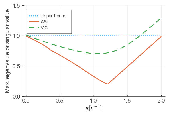
Using these compound plant parameters, we determine the spectral radius and the maximum singular value as given in (24) and (25) for a large number of values of the learning gain $\kappa\in[0,2]\,\text{h}^{-1}$. The resulting design plot is presented in Figure 3. We can assure asymptotic stability in the iteration domain for $\kappa\in(0,2]\,\text{h}^{-1}$ and monotonic convergence of the error for $\kappa\in[0.025,1.6775]\,\text{h}^{-1}$. Furthermore, we predict that the fastest learning dynamics are achieved by a learning gain $\kappa=1.205\,\text{h}^{-1}$ with a spectral radius of $0.205$. For the sake of robustness, we choose a slightly smaller value, $\kappa=1\,\text{h}^{-1}$, for which the spectral radius is clearly below $0.5$.

References

- Aamir et al. (2016) Aamir, M., Kalwar, K.A., and Mekhilef, S. (2016). Uninterruptible power supply (UPS) system. Renewable and sustainable energy reviews, 58, 1395–1410.
- Bampoulas et al. (2019) Bampoulas, A., Saffari, M., Pallonetto, F., Mangina, E., and Finn, D.P. (2019). Self-learning control algorithms for energy systems integration in the residential building sector. In 2019 IEEE 5th World Forum on Internet of Things (WF-IoT), 815–818. IEEE.
- Bidram and Davoudi (2012) Bidram, A. and Davoudi, A. (2012). Hierarchical structure of microgrids control system. IEEE Transactions on Smart Grid, 3(4), 1963–1976.
- Bristow et al. (2006) Bristow, D.A., Tharayil, M., and Alleyne, A.G. (2006). A survey of iterative learning control. IEEE control systems magazine, 26(3), 96–114.
- Chai et al. (2016) Chai, B., Yang, Z., Gao, K., and Zhao, T. (2016). Iterative learning for optimal residential load scheduling in smart grid. Ad Hoc Networks, 41, 99–111.
- Doh (1999) Doh, T.Y. (1999). Robust iterative learning control with current feedback for uncertain linear systems. International Journal of Systems Science, 30(1), 39–47.
- Dörfler et al. (2014) Dörfler, F., Simpson-Porco, J.W., and Bullo, F. (2014). Plug-and-play control and optimization in microgrids. In 53rd IEEE Conference on Decision and Control, 211–216. IEEE.
- Fünfgeld and Tiedemann (cited Oct 2019) Fünfgeld, C. and Tiedemann, R. (cited Oct 2019). Bundesverband der Energie- und Wasserwirtschaft Website. www.bdew.de/energie/standardlastprofile-strom.
- Guerrero et al. (2010) Guerrero, J.M., Vasquez, J.C., Matas, J., De Vicuña, L.G., and Castilla, M. (2010). Hierarchical control of droop-controlled AC and DC microgrids - A general approach toward standardization. IEEE Transactions on industrial electronics, 58(1), 158–172.
- Guo et al. (2019) Guo, H.q., Liu, C.z., Yong, J.w., Cheng, X.q., and Muhammad, F. (2019). Model predictive iterative learning control for energy management of plug-in hybrid electric vehicle. IEEE Access.
- Guo et al. (2015) Guo, W., Liu, F., Si, J., He, D., Harley, R., and Mei, S. (2015). Online supplementary ADP learning controller design and application to power system frequency control with large-scale wind energy integration. IEEE transactions on neural networks and learning systems, 27(8), 1748–1761.
- Han et al. (2016) Han, Y., Li, H., Shen, P., Coelho, E.A.A., and Guerrero, J.M. (2016). Review of active and reactive power sharing strategies in hierarchical controlled microgrids. IEEE Transactions on Power Electronics, 32(3), 2427–2451.
- Hellmann et al. (2018) Hellmann, F., Schultz, P., Jaros, P., Levchenko, R., Kapitaniak, T., Kurths, J., and Maistrenko, Y. (2018). Network-induced multistability: Lossy coupling and exotic solitary states. arXiv preprint arXiv:1811.11518.
- Jang et al. (1995) Jang, T.J., Choi, C.H., and Ahn, H.S. (1995). Iterative learning control in feedback systems. Automatica, 31(2), 243–248.
- Jian-Xin (2005) Jian-Xin, X. (2005). Recent advances in iterative learning control. 自动化学报 , 31(1), 132–142.
- Li et al. (2015) Li, X., Xu, J.X., and Huang, D. (2015). Iterative learning control for nonlinear dynamic systems with randomly varying trial lengths. International Journal of Adaptive Control and Signal Processing, 29(11), 1341–1353.
- Li et al. (2017) Li, Z., Zang, C., Zeng, P., Yu, H., and Li, S. (2017). Fully distributed hierarchical control of parallel grid-supporting inverters in islanded AC microgrids. IEEE Transactions on Industrial Informatics, 14(2), 679–690.
- Liu and Ruan (2016) Liu, J. and Ruan, X. (2016). Networked iterative learning control approach for nonlinear systems with random communication delay. International Journal of Systems Science, 47(16), 3960–3969.
- Machowski et al. (2011) Machowski, J., Bialek, J., and Bumby, J. (2011). Power system dynamics: Stability and control. John Wiley & Sons, Ltd.
- Merris (1994) Merris, R. (1994). Laplacian matrices of graphs: A survey. Linear algebra and its applications, 197, 143–176.
- Nguyen and Banjerdpongchai (2016) Nguyen, D.H. and Banjerdpongchai, D. (2016). Iterative learning control of energy management system: Survey on multi-agent system framework. Engineering Journal, 20(5), 1–4.
- Olivares et al. (2014) Olivares, D.E., Mehrizi-Sani, A., Etemadi, A.H., Cañizares, C.A., Iravani, R., Kazerani, M., Hajimiragha, A.H., Gomis-Bellmunt, O., Saeedifard, M., Palma-Behnke, R., et al. (2014). Trends in microgrid control. IEEE Transactions on smart grid, 5(4), 1905–1919.
- Pan et al. (2006) Pan, Y.J., Marquez, H.J., and Chen, T. (2006). Sampled-data iterative learning control for a class of nonlinear networked control systems. In 2006 American Control Conference, 6–pp. IEEE.
- Paszke et al. (2016) Paszke, W., Rogers, E., and Gałkowski, K. (2016). Experimentally verified generalized KYP lemma based iterative learning control design. Control Engineering Practice, 53, 57–67.
- Rackauckas and Nie (2017) Rackauckas, C. and Nie, Q. (2017). Differentialequations. jl–a performant and feature-rich ecosystem for solving differential equations in julia. Journal of Open Research Software, 5(1).
- Roover et al. (2000) Roover, D.D., Bosgra, O.H., and Steinbuch, M. (2000). Internal-model-based design of repetitive and iterative learning controllers for linear multivariable systems. International Journal of Control, 73(10), 914–929.
- Schiffer et al. (2015) Schiffer, J., Zonetti, D., Ortega, R., Stankovic, A., Sezi, T., and Raisch, J. (2015). Modeling of microgrids - from fundamental physics to phasors and voltage sources. Automatica, 1–15.
- Seel et al. (2013) Seel, T., Weber, S., Affeld, K., and Schauer, T. (2013). Iterative learning cascade control of continuous noninvasive blood pressure measurement. In IEEE International Conference on Systems, Man, and Cybernetics, 2207–2212. Manchester, UK.
- Serrani et al. (2001) Serrani, A., Isidori, A., and Marconi, L. (2001). Semi-global nonlinear output regulation with adaptive internal model. IEEE Transactions on Automatic Control, 46(8), 1178–1194.
- Shen et al. (2017) Shen, D., Zhang, C., and Xu, Y. (2017). Two updating schemes of iterative learning control for networked control systems with random data dropouts. Information Sciences, 381, 352–370.
- Stott et al. (2009) Stott, B., Jardim, J., and Alsac, O. (2009). DC Power Flow Revisited. IEEE Transactions on Power Systems, 24(3), 1290–1300.
- Strenge et al. (2020) Strenge, L., Schultz, P., Kurths, J., Raisch, J., and Hellmann, F. (2020). A multiplex, multi-timescale model approach for economic and frequency control in power grids. Chaos: An Interdisciplinary Journal of Nonlinear Science, 30(3), 033138.
- Teng (2014) Teng, K.T. (2014). Repetitive and iterative learning control for power converter and precision motion control. Ph.D. thesis, UCLA.
- Wanner and Hairer (1996) Wanner, G. and Hairer, E. (1996). Solving ordinary differential equations II. Springer Berlin Heidelberg.
- Weitenberg et al. (2018) Weitenberg, E., Jiang, Y., Zhao, C., Mallada, E., Dörfler, F., and De Persis, C. (2018). Robust decentralized frequency control: A leaky integrator approach. In 2018 European Control Conference (ECC), 764–769.
- Xin et al. (2015) Xin, H., Zhao, R., Zhang, L., Wang, Z., Wong, K.P., and Wei, W. (2015). A decentralized hierarchical control structure and self-optimizing control strategy for FP type DGs in islanded microgrids. IEEE Transactions on Smart Grid, 7(1), 3–5.
- Xu et al. (2006) Xu, J.X., Yan, R., and Chen, Y. (2006). On initial conditions in iterative learning control. In 2006 American Control Conference, 6–pp. IEEE.
- Xu and Yang (2013) Xu, J.X. and Yang, S. (2013). Iterative learning based control and optimization for large scale systems. IFAC Proceedings Volumes, 46(13), 74–81.
- Yan et al. (2010) Yan, X., Ren, Q., and Meng, Q. (2010). Iterative learning control in large scale HVAC system. In 2010 8th World Congress on Intelligent Control and Automation, 5063–5066. IEEE.
- Zeng et al. (2013) Zeng, Z., Yang, H., Zhao, R., and Cheng, C. (2013). Topologies and control strategies of multi-functional grid-connected inverters for power quality enhancement: A comprehensive review. Renewable and Sustainable Energy Reviews, 24, 223–270.
Appendix A Demand model
A.1 Synthetic demand model
As a benchmark for the proposed ILC control, we consider synthetic demand curves. For every node in the network, the demand is dominated by a periodic baseline (see Fig. 7, left):
where the period [s] is the duration of a day and the demand amplitudes [W/W] are uniform i.i.d. random numbers. At the beginning of each hour in cycle , the nodal demands are updated as