Detecting chiral pairing and topological superfluidity using circular dichroism

The realisation and manipulation of topological superfluids and superconductors is presently one of the most actively pursued goals in physics. In addition to being interesting from a fundamental science point of view, their Majorana edge modes promise applications for quantum computing Nayak et al. 2008. Zero-energy states at the ends of one-dimensional (1D) nanowires have been observed, consistent with the presence of Majorana modes Nadj-Perge et al. 2014; Lutchyn et al. 2018. So far, there has however been no observation of topological superfluidity in 2D. The most promising solid-state candidate for a 2D topological superconductor is Sr₂RuO₄, but the precise symmetry of the order parameter in this crystal remains subject to intense debate Hicks et al. 2010; Mackenzie et al. 2017; Kivelson et al. 2020. It has recently been shown that an atomic 2D Fermi gas immersed in a BEC offers a promising platform for realising a topological superfluid Wu and Bruun 2016; Midtgaard et al. 2016; Midtgaard et al. 2017. The fermions form Cooper pairs with chiral symmetry by exchanging sound modes in the BEC, and the system offers sufficient flexibility so that one can tune the superfluid critical temperature to be within experimental reach. Experimentally, such a Bose-Fermi mixture has been realized using ¹⁷³Yb-⁷Li atoms, which constitutes an important step towards the first unequivocal realisation of a topological $p_{x}\!+\!ip_{y}$ superfluid Schäfer et al. 2018.

A key question concerns the detection of topological superfluidity in atomic gases. Their topological properties are not easily extracted from thermodynamic measurements nor using common probes such as radio-frequency spectroscopy Grosfeld et al. 2007. Contrary to the chiral edge modes of single-particle band structures, which have been detected in experiments Cooper et al. 2019, the observation of Majorana states Möller et al. 2011; Gong et al. 2012 is complicated by their small number and their particle-hole nature.

It was recently proposed Tran et al. 2017; Tran et al. 2018 and experimentally demonstrated Asteria et al. 2019 that the topologically invariant Chern number can be detected in atomic gases through circular dichroism, namely, by analyzing excitation rates upon applying a circular drive. This topological probe was first introduced for non-interacting Chern insulators Tran et al. 2017, and later applied to interacting many-body systems Schüler and Werner 2017; Repellin and Goldman 2019; Klein et al. 2020. Inspired by this approach, we hereby demonstrate that the chirality of the $p_{x}\!+\!ip_{y}$ pairing is revealed in the circular dichroism of the superfluid. For weak pairing, the differential excitation rate obtained from opposite drive orientations, integrated over the drive frequency, is shown to be determined by the Chern number of the topological superfluid, in direct analogy with Chern insulators Tran et al. 2017. However, in contrast with the latter case, a non-topological contribution scaling as the superfluid gap squared becomes significant for strong pairing. The resulting competition between maximising the superfluid critical temperature while detecting a genuine topological signature is analysed for a concrete atomic Bose-Fermi mixture. Using the strong-coupling Eliasberg equations combined with Berezinskii-Kosterlitz-Thouless (BKT) theory, we identify a wide and accessible parameters regime where the superfluid critical temperature is high and the dichroic signal dominated by the topological Chern number. Our results demonstrate that the dichroic probe offers an experimentally promising pathway to detect topological superfluidity.

We first establish a connection between circular dichroism, the Hall conductivity, and the Chern number of the superfluid. Consider a 2D system of spin-polarised fermions described by the Hamiltonian

	$$\displaystyle H_{0}=\int d^{2}r\,\psi^{\dagger}({\mathbf{r}})\left(-\frac{\nabla^{2}}{2m}\right)\psi({\mathbf{r}})$$
	$$\displaystyle+\frac{1}{2}\iint d^{2}rd^{2}r^{\prime}\,\psi^{\dagger}({\mathbf{r}})\psi^{\dagger}({\mathbf{r}}^{\prime})V({\mathbf{r}}-{\mathbf{r}}^{\prime})\psi({\mathbf{r}}^{\prime})\psi({\mathbf{r}}),$$		(1)

where $\psi({\mathbf{r}})$ is the fermion field and $V({\mathbf{r}}-{\mathbf{r}}^{\prime})$ is an interaction giving rise to pairing, which may result from a $p$-wave Feshbach resonance or, as we will consider later, from an induced interaction. Within BCS theory, this $p$-wave superfluid can be described by the Hamiltonian

$\displaystyle H_{\rm BCS}=\sum_{\bf k}\Phi_{\bf k}^{\dagger}H_{\bf k}\Phi_{\bf k},\quad H_{\mathbf{k}}={\mathbf{h}}_{\mathbf{k}}\cdot\bm{\tau},$

(2)

where $\Phi_{\bf k}\equiv[a_{\bf k},a^{\dagger}_{-{\bf k}}]^{T}$, ${\mathbf{h}}_{\mathbf{k}}=(\text{Re}\Delta_{\mathbf{k}},-\text{Im}\Delta_{\mathbf{k}},\xi_{\bf k})^{T}$ and where $\bm{\tau}=(\tau_{1},\tau_{2},\tau_{3})^{T}$ with $\tau_{i}$ the Pauli matrices. Here $\xi_{\bf k}=k^{2}/2m-\mu$, where $\mu$ is the chemical potential, and $\Delta_{\bf k}$ is the gap parameter ($\hbar\!=\!1$ throughout). The latter is taken to have chiral $p$-wave symmetry, i.e. $\Delta_{\mathbf{k}}=\Delta_{k}e^{i\phi}$, where $\phi$ is the polar angle of the momentum ${\mathbf{k}}$ and $k=|\mathbf{k}|$, since this gives the lowest energy for $p$-wave pairing as it have no nodes Anderson and Morel 1961; Lu and Barford 1991. Indeed, as $\Delta_{k}\propto k$ for $k\ll k_{F}$ due to Fermi anti-symmetry, we get $\Delta_{\mathbf{k}}\propto k_{x}+ik_{y}$. This results in a topological phase characterised by a Chern number $C\!=\!-1$ for $\mu>0$ whereas $C\!=\!0$ for $\mu<0$ Read and Green 2000. The Chern number reads

		$\displaystyle C=\int\!\frac{d^{2}k}{4\pi}\frac{1}{|\mathbf{h_{k}}|^{3}}\mathbf{h_{k}}\cdot\partial_{k_{x}}{\mathbf{h}}\times\partial_{k_{y}}{\mathbf{h}}$		(3)
		$\displaystyle=\int\!\frac{d^{2}k}{2\pi}\left[\frac{v_{x}}{E_{\mathbf{k}}^{3}}\text{Im}(\Delta^{*}_{\mathbf{k}}\partial_{k_{y}}\Delta_{\mathbf{k}})+\frac{\xi_{\mathbf{k}}}{2E_{\mathbf{k}}^{3}}\text{Im}(\partial_{k_{x}}\Delta_{\mathbf{k}}\partial_{k_{y}}\Delta^{*}_{\mathbf{k}})\right],$

where $v_{x}=k_{x}/m$ and $E_{\mathbf{k}}=\sqrt{\xi_{\mathbf{k}}^{2}+|\Delta_{\mathbf{k}}|^{2}}$ is the BCS quasiparticle energy. The second term in the integrand scales as $\Delta_{\mathbf{k}}^{2}/\mu^{2}$ so that the Chern number can be approximated by the first term in the regime $\Delta_{\mathbf{k}}\ll\mu$.

We now show that the Chern number in Eq. (3) can be extracted from circular dichroism, namely, by monitoring excitation rates upon a circular drive Tran et al. 2017; Asteria et al. 2019. We consider a circular drive of the form

$\displaystyle V_{\pm}(\mathbf{r};\mathbf{q})$

$\displaystyle=2\mathcal{E}\left(x\cos\Omega t\pm y\sin\Omega t\right)\cos{{\bf q}\cdot{\bf r}},$

(4)

and we will set ${\bf q}\!\rightarrow 0$ at the end of calculations, corresponding to a uniform circular shaking Asteria et al. 2019. This reads

$\displaystyle V_{\pm}(\mathbf{q})=\frac{\mathcal{E}}{i}\left[-\frac{\partial\tilde{n}({\bf q})}{\partial q_{x}}\pm i\frac{\partial\tilde{n}({\bf q})}{\partial q_{y}}\right]e^{-i\Omega t}+\text{h.c.},$

(5)

in second quantization, where $n(\mathbf{r})=\psi^{\dagger}({\mathbf{r}})\psi({\mathbf{r}})$ is the density operator, $n({\bf q})$ is its Fourier transform and $\tilde{n}({\bf q})=[n({\bf q})-n(-{\bf q})]/2$. Within linear response, the excitation rate out of the ground state of $H_{0}$ induced by $V_{\pm}(\mathbf{q})$ can be calculated using Fermi’s golden rule as

	$\displaystyle\Gamma_{\pm}(\mathbf{q},\Omega)=$	$\displaystyle 2\pi{\mathcal{E}^{2}}\sum_{f}\left|\left\langle f\left|\frac{\partial\tilde{n}({\bf q})}{\partial q_{x}}\pm i\frac{\partial\tilde{n}({\bf q})}{\partial q_{y}}\right|g\right\rangle\right|^{2}$
		$\displaystyle\times\delta(E_{f}-E_{g}-\Omega),$		(6)

where $|g\rangle$ and $|f\rangle$ denote the ground and excited states of $H_{0}$ with energy $E_{g}$ and $E_{f}$, respectively.

The observable of interest is provided by the differential integrated rate (DIR), which is defined as Tran et al. 2017

$\displaystyle\Delta\Gamma=\lim_{{\bf q}\rightarrow 0}\frac{1}{2}\int_{0}^{\infty}\!d\Omega[\Gamma_{+}(\mathbf{q},\Omega)-\Gamma_{-}(\mathbf{q},\Omega)].$

(7)

Substituting Eq. (6) into Eq. (7), we find

$\displaystyle\Delta\Gamma$

$\displaystyle=-\pi i\mathcal{E}^{2}\lim_{{\bf q}\rightarrow 0}\left\langle g\left|\left[\frac{\partial n({\bf q})}{\partial q_{x}},\frac{\partial n(-{\bf q})}{\partial q_{y}}\right]\right|g\right\rangle,$

(8)

where we have used momentum conservation to eliminate terms. We now use the continuity equation to write $\Delta\Gamma$ in terms of the density-current correlation function. From $\partial_{t}n({\bf r},t)+\nabla\cdot{\bf j}({\bf r},t)=0$, we find

$\displaystyle\langle g|n({\bf q})|f\rangle=\frac{\langle g|{\bf q}\cdot{\bf j}({\bf q})|f\rangle}{E_{f}-E_{g}},$

(9)

where the Fourier transform of the current reads

$\displaystyle{\bf j}({\bf q})\!=\!(1/2mi)\int d^{2}re^{-i{\bf q}\cdot{\bf r}}[\psi^{\dagger}({\mathbf{r}})\nabla\psi({\mathbf{r}})\!-\!\text{h.c.}].$

(10)

Using Eqs. (8)-(9) and noting that

$\displaystyle\lim_{q_{y}\rightarrow 0}\lim_{q_{x}\rightarrow 0}\langle g|{\partial_{q_{y}}n({\bf q})}|f\rangle=\lim_{q_{y}\rightarrow 0}\lim_{q_{x}\rightarrow 0}\langle g|{n({\bf q})}/{q_{y}}|f\rangle,$

(11)

we find the relation

$\displaystyle\Delta\Gamma/\mathcal{A}=2\pi\mathcal{E}^{2}\sigma_{xy},$

(12)

which connects the DIR to the static Hall conductivity

	$\displaystyle\sigma_{xy}$	$\displaystyle\equiv\lim_{q_{y}\rightarrow 0}\lim_{q_{x}\rightarrow 0}\lim_{\omega\rightarrow 0}\frac{1}{i\mathcal{A}\omega}\chi_{j_{x},j_{y}}({\bf q},\omega)$
		$\displaystyle=\lim_{q_{y}\rightarrow 0}\lim_{q_{x}\rightarrow 0}\lim_{\omega\rightarrow 0}\frac{1}{i\mathcal{A}q_{y}}{\chi_{j_{x},n}({\bf q},\omega)}.$		(13)

Here $\mathcal{A}$ is the system’s area, and $\chi_{A,B}(\mathbf{q},\omega)$ is the Fourier transform of the retarded correlation function

$\displaystyle\chi_{A,B}(\mathbf{q},t-t^{\prime})=-i\theta(t-t^{\prime})\left\langle[A(\mathbf{q},t),B(-\mathbf{q},t^{\prime})]\right\rangle,$

(14)

with $\theta(x)$ the Heaviside function. We note that the specific order of limits (taking $\omega\!\rightarrow\!0$ before ${\bf q}\!\rightarrow\!0$) is crucial, since the more standard order $\lim_{\omega\rightarrow 0}\lim_{{\bf q}\rightarrow 0}\frac{1}{i\omega}\chi_{j_{x},j_{y}}({\bf q},\omega)$ yields zero for a translationally invariant system Giuliani and Vignale 2005; this subtlety also arises when analysing edge currents Volovik 1992; Volovik 1988; Goryo and Ishikawa 1998; Stone and Roy 2004.

Besides, Eq. (12) was obtained by taking the finite nature of realistic systems into account. In particular, one would obtain an additional factor of $1/2$ for a strictly translationally invariant system. Indeed, when deriving Eq. (8), we use that $\langle A({\mathbf{q}}),B(\mathbf{q}^{\prime})\rangle\propto\delta_{\mathbf{q},-\mathbf{q}^{\prime}}$ for a strictly infinite translationally invariant system. From this, it follows that $\lim_{\mathbf{q}\rightarrow 0}\langle n(\mathbf{q})n(\mathbf{q})\rangle=0$ and such terms can be discarded. However, for a finite physical system of size $L$, momentum is only defined with a resolution $\sim 1/L$. This means that $\langle n(\mathbf{q})n(\mathbf{q})\rangle$ starts to become non-zero for $q\lesssim 1/L$ and in particular $\lim_{\mathbf{q}\rightarrow 0}\langle n(\mathbf{q})n(\mathbf{q})\rangle=\langle n(\mathbf{0})n(\mathbf{0})\rangle$ for a finite system, which leads to the extra factor of $2$ on the right hand side of Eq. (12). Physically, it means that a finite system cannot distinguish between a force with wave length much greater than the system size from a uniform force. We note that uniform circular shaking ($\mathbf{q}\!=\!0$) can be realized in ultracold-atom experiments. We also point out that Eq. (12) is universal: it can also be derived from Kramers-Kronig relations Tran et al. 2017; Repellin and Goldman 2019; Bennett and Stern 1965; Souza and Vanderbilt 2008, noting that the excitation rates $\Gamma_{\pm}(\Omega)$ are related to the power absorbed upon the circular drive $P_{\pm}(\Omega)=\Omega\Gamma_{\pm}(\Omega)$.

The Hall conductivity of a superfluid was previously shown to be related to a Chern number; see Refs. Volovik 1992; Volovik 1988 in the context of chiral ³He superfluids. Using BCS theory, the current-density correlation function can be written as Mahan 2000

$$\chi_{j_{x},n}(q)=-\sum_{k}\frac{k_{x}}{2m}\text{tr}\left[\mathcal{G}_{0}(k-q/2)\mathcal{G}_{0}(k+q/2)\tau_{3}\right]$$

(15)

where in shorthand notation $k=(\mathbf{k},\omega_{n})$ with $\omega_{n}$ a fermionic Matsubara frequency, and $\mathcal{G}_{0}$ is the BCS Green’s function. We have

$$\mathcal{G}_{0}(k)=\int_{-\infty}^{\infty}\frac{d\omega}{(-\pi)}\frac{\text{Im}\mathcal{G}_{0}(\mathbf{k},\omega)}{i\omega_{n}-\omega}$$

(16)

where

	$\displaystyle\text{Im}\mathcal{G}_{0}(\mathbf{k},\omega)=$	$\displaystyle-\frac{\pi}{2E_{\mathbf{k}}}\begin{pmatrix}\omega+\xi_{\mathbf{k}}&-\Delta_{\mathbf{k}}\\ -\Delta_{\mathbf{k}}^{\ast}&\omega-\xi_{\mathbf{k}}\end{pmatrix}$
		$\displaystyle\times\left[\delta(\omega-E_{\mathbf{k}})-\delta(\omega+E_{\mathbf{k}})\right].$		(17)

Inserting this in Eq. (15) and performing the Matsubara sum yields to first order in $\mathbf{q}$

	$\displaystyle\lim_{\omega\to 0}\chi_{j_{x},n}(\mathbf{q},\omega)=$	$\displaystyle-\frac{iq_{x}}{\mathcal{V}}\sum_{\mathbf{k}}\frac{k_{x}}{2m}\frac{\text{Im}\Delta_{\mathbf{k}}\partial_{k_{x}}\Delta_{\mathbf{k}}^{\ast}}{E_{\mathbf{k}}^{3}}$
		$\displaystyle-\frac{iq_{y}}{2\mathcal{V}}\sum_{\mathbf{k}}\frac{k_{x}}{2m}\frac{\text{Im}\Delta_{\mathbf{k}}\partial_{k_{y}}\Delta_{\mathbf{k}}^{\ast}}{E_{\mathbf{k}}^{3}}.$		(18)

The first of these terms vanish, since the summand is odd in $k_{y}$. This can be seen if we fix the phase of the gap function and look at, for instance, the simple example $\Delta_{\mathbf{k}}=k_{x}+ik_{y}$. With this, it is clear that

	$\displaystyle\lim_{{\mathbf{q}}\rightarrow 0}\lim_{\omega\to 0}\frac{\chi_{j_{x},n}({\mathbf{q}},\omega)}{iq_{y}}$	$\displaystyle=\int\!\frac{d^{2}\mathbf{k}}{8\pi^{2}}\frac{k_{x}}{m}\frac{\text{Im}[\Delta_{\mathbf{k}}^{*}\partial_{k_{y}}\Delta_{\mathbf{k}}]}{E_{\mathbf{k}}^{3}}$
		$\displaystyle=\frac{C}{4\pi}+\mathcal{O}(\Delta^{2}/\mu^{2}),$		(19)

where the last equality is obtained by comparing with the Chern number in Eq. (3). In contrast with the case of Chern insulators, where the Hall conductivity is genuinely topological in the thermodynamic limit Thouless et al. 1982, the Hall response of the superfluid [Eq. (19)] contains a correction scaling as $\mathcal{O}(\Delta^{2}/\mu^{2})$. This result was previously related to the fact that the edge current of a chiral $p$-wave superconductor is not strictly topological, as opposed to the presence of edge (Majorana) states Taylor and Kallin 2012; Huang et al. 2014; Huang et al. 2015.

Finally, combining Eqs. (12) and (19) yields the central result of this work,

$\displaystyle\Delta\Gamma/\mathcal{A}=(1/2)\,\mathcal{E}^{2}C+\mathcal{O}(\Delta^{2}/\mu^{2}),$

(20)

which shows that the DIR related to the dichroic probe is closely related to the Chern number of the superfluid phase: this observable exhibits a jump proportional to the Chern number to order $\mathcal{O}(\Delta^{2}/\mu^{2})$ whenever the superfluid enters the topological phase with $C=-1$.

We now explore the dichroic probe for a concrete system consisting of a 2D gas of fermionic atoms immersed in a 3D BEC. The fermions interact by exchanging sound modes in the BEC, which leads to an induced attractive interaction and Cooper pairing Wu and Bruun 2016. Since both the range and strength of the induced interaction can be varied, one can tune the mixture in order to reach a high critical temperature. This makes such a mixture a strong candidate for observing a chiral pairing. Recently, progress towards realising this goal was reported with the experimental realisation of a ¹⁷³Yb-⁷Li mixture Schäfer et al. 2018. We now analyse how the dichroic probe can be used to detect topological pairing in this specific system.

Due to the finite speed of sound in the BEC, the interaction between the fermions mediated by the bosons is not instantaneous, thus giving rise to retardation effects. The latter are included in the frequency-dependent Eliashberg equations as explained in the appendix. It has been shown that retardation effects are small when the bosons in the BEC are light compared to the fermions such as for the ¹⁷³Yb-⁷Li mixture Kinnunen et al. 2018. The induced interaction is then close to the static Yukawa form

$$V(\mathbf{r})=-\frac{a_{\rm eff}^{2}n_{B}m_{B}}{\pi}\frac{\exp(-\sqrt{2}r/\xi_{B})}{r}.$$

(21)

Here, $n_{B}$ and $m_{B}$ is the density and mass of the bosons, $\xi_{B}=1/\sqrt{8\pi n_{B}a_{B}}$ is the BEC healing length with $a_{B}$ the boson-boson scattering length, and $a_{\rm eff}$ is the mixed dimensional Bose-Fermi scattering length.

According to Eq. (7), one should measure the differential rate $\Gamma_{+}-\Gamma_{-}$ integrated over all frequencies. However, any real measurement necessarily introduces an upper cut-off frequency $\Omega_{c}$ above which there is no signal Asteria et al. 2019. Using Eqs. (12) and (19), the resulting signal reads

$$\frac{\Delta\Gamma_{\text{trunc}}(\Omega_{c})}{\mathcal{A}\mathcal{E}^{2}}\!\equiv\!\int\!\frac{d^{2}k}{4\pi}\frac{k_{x}}{m}\frac{\text{Im}[\Delta_{\mathbf{k}}^{*}\partial_{k_{y}}\Delta_{\mathbf{k}}]}{E_{\mathbf{k}}^{3}}\theta(\Omega_{c}-2E_{\mathbf{k}})$$

(22)

The cut-off $\theta(\Omega_{c}-2E_{\mathbf{k}})$ reflects that the probe breaks pairs with energy $2E_{\mathbf{k}}$ in the long wave length limit. We note that $\Delta\Gamma\!=\!\lim_{\Omega_{c}\to\infty}\Delta\Gamma_{\text{trunc}}(\Omega_{c})$.

In Fig. 1, we plot $\Delta\Gamma_{\text{trunc}}(\Omega_{c})$ for a ⁷Li-¹⁷³Yb mixture with a Bose-Fermi coupling $n_{B}^{1/3}a_{\rm eff}=0.12$, BEC gas parameter $n_{B}^{1/3}a_{B}=0.1$, and density ratio $n_{F}^{1/2}/n_{B}^{1/3}=0.5$, where $n_{F}$ is the 2D Fermi density. These results are obtained by first solving the BCS equations self-consistently at zero temperature and then evaluating the DIR from Eq. (22). The numerical solution indeed confirms the $p$-wave form of pairing $\Delta_{\bf k}=\Delta_{k}e^{i\phi}$ where $\Delta_{k}\propto k$ for small momenta.

The DIR is zero for cut-off frequencies below twice the gap, i.e. for $\Omega_{c}\lesssim 0.1E_{F}$ where $E_{F}$ is the 2D Fermi energy, reflecting that there is not enough energy in the probe to break pairs. Above this threshold, the DIR quickly converges towards to the Chern number for $\Omega_{c}\gtrsim E_{F}$. Since $\Delta\simeq 0.05E_{F}\ll E_{F}$ for this set of parameters, the deviation of $2\Delta\Gamma/\mathcal{AE}^{2}$ away from the Chern number is small. We also plot in Fig. 1 the differential rate at a given frequency $\Omega$,

$\displaystyle\frac{1}{2}[\Gamma_{+}(\Omega)-\Gamma_{-}(\Omega)]=\frac{\partial}{\partial\Omega}\Delta\Gamma_{\text{trunc}}(\Omega).$

(23)

This difference is large for frequencies just above the threshold given by twice the gap, where the density of states of the superfluid is highest, and Fig. 1 shows that that one only needs to measure the difference up to a few times the pairing gap to resolve the Chern number.

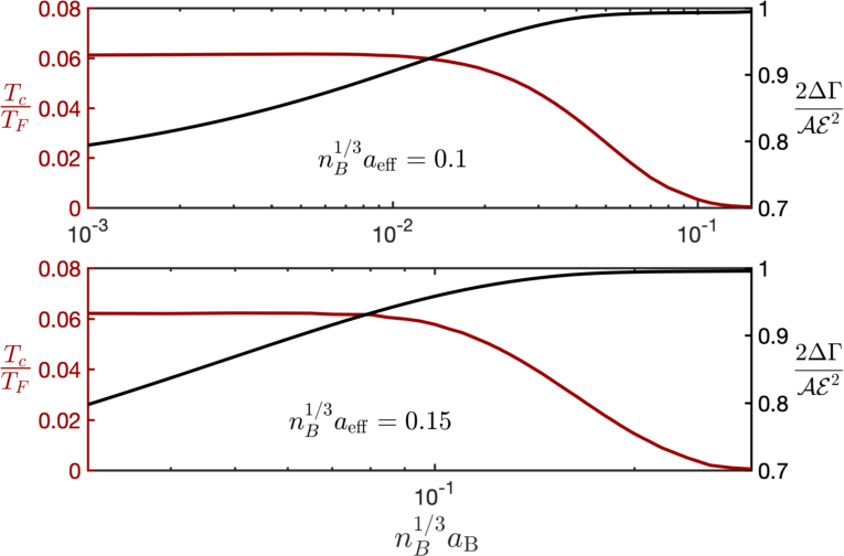
One of the appealing features of the Bose-Fermi mixture is that the critical temperature for the 2D superfluid can be tuned to be close to the maximum value $T_{c}/T_{F}=1/16$ allowed by BKT theory. Maximising $T_{c}$ will however also increase the gap and thereby increase corrections to the DIR away from the Chern number as seen from Eq. (20). To analyse this tension, we plot in Fig. 2 the DIR $\Delta\Gamma$ at zero temperature and the critical temperature $T_{c}$ as a function of the gas parameter $n_{B}^{1/3}a_{\text{\rm B}}$ for $n_{F}^{1/2}/n_{B}^{1/3}=0.5$ and two different Bose-Fermi interaction strengths. The critical temperature is calculated by combining strong coupling Eliashberg and BKT theory, which includes the frequency dependence of the gap; see Refs. Wu and Bruun 2016 and the appendix for details. We see that the critical temperature increases with decreasing gas parameter reflecting that the range of interaction in Eq. (21), given by the BEC coherence length, increases. The gap consequently also increases leading to a larger correction term for the DIR away from $\Delta\Gamma\!=\!\mathcal{AE}^{2}{\mathcal{C}}/2$. Nevertheless, Fig. 2 shows that there is a significant region where both the DIR is close to the topological value and the critical temperature is close to its maximum value $T_{c}/T_{F}=1/16$. Note that we expect our calculation to give a lower bound on the DIR, since BCS theory likely overestimates the gap.

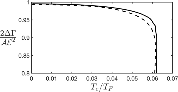
To further illustrate the competition between maximising the critical temperature and measuring a value of $\Delta\Gamma$ determined by the underlying topology, we plot $\Delta\Gamma$ at zero temperature as a function of $T_{c}$ in Fig. 3 for the same parameters as in Fig. 2. This demonstrates that in order for the dichroic probe to yield a value close to that given by the Chern number, one should cool to around $T\sim 0.06E_{F}$. Since temperatures down to $T\simeq 0.03E_{F}$ have been obtained for 2D Fermi gases Luick et al. 2019; Sobirey et al. 2020; Ries et al. 2015, this is within present day technology making our scheme promising for detecting topological superfluidity. It also shows that a stronger Bose-Fermi interaction strength is slightly more favorable although the difference between the two interaction strengths is small.

For $T=0$, BCS theory has been shown to be surprisingly accurate even for strong coupling where the Cooper pairs are tightly bound and the system is in the so-called BEC regime Pieri et al. 2005. It follows that our calculation of the DIR is reliable even in this regime, where the correction term $\mathcal{O}(\Delta^{2}/\mu^{2})$ away from the quantized value is large. Any non-zero value however indicates chiral pairing, since the DIR is zero in a phase with time-reversal symmetry. Our scheme thus provides a way to observe the topological phase transition to a trivial phase when $\mu$ becomes negative deep in the BEC regime.

We showed that chiral $p_{x}+ip_{y}$ pairing in a 2D superfluid can be detected through circular dichroism. Contrary to the case of topological insulators Tran et al. 2017, the DIR is not purely dictated by the Chern number due to a correction term scaling as $\Delta^{2}/E_{F}^{2}$, giving rise to a competition between maximising the critical temperature of the superfluid and observing the Chern number from such a dichroic probe. As a concrete example, we considered an atomic Bose-Fermi mixture. Using a combination of Eliashberg and BKT theory, it was demonstrated that there is in fact a wide range of values for the system parameters where both the critical temperature is high and the dichroic signal close to the value given by the Chern number. This combined with the fact that a similar scheme was recently successfully applied to detect topological order in a Chern Bloch band Asteria et al. 2019, leads to the conclusion that the dichroic probe is a strong candidate for detecting topological $p_{x}+ip_{y}$ pairing in an atomic system.

Acknowledgements.— J.M.M. and G.M.B. wish to acknowledge the support of the Danish Council of Independent Research – Natural Sciences via Grant No. DFF - 4002-00336. Z.W. acknowledges the support by the National Science Foundation of China (Grant No.11904417) and the Key-Area Research and Development Program of GuangDong Province (Grant No.2019B030330001). N.G. is supported by the ERC Starting Grant TopoCold, and the Fonds De La Recherche Scientifique (FRS-FNRS, Belgium).

References

- Nayak et al. (2008) C. Nayak, S. H. Simon, A. Stern, M. Freedman, and S. Das Sarma, Rev. Mod. Phys. 80, 1083 (2008).
- Nadj-Perge et al. (2014) S. Nadj-Perge, I. K. Drozdov, J. Li, H. Chen, S. Jeon, J. Seo, A. H. MacDonald, B. A. Bernevig, and A. Yazdani, Science 346, 602 (2014), https://science.sciencemag.org/content/346/6209/602.full.pdf .
- Lutchyn et al. (2018) R. M. Lutchyn, E. P. A. M. Bakkers, L. P. Kouwenhoven, P. Krogstrup, C. M. Marcus, and Y. Oreg, Nature Reviews Materials 3, 52 (2018).
- Hicks et al. (2010) C. W. Hicks, J. R. Kirtley, T. M. Lippman, N. C. Koshnick, M. E. Huber, Y. Maeno, W. M. Yuhasz, M. B. Maple, and K. A. Moler, Phys. Rev. B 81, 214501 (2010).
- Mackenzie et al. (2017) A. P. Mackenzie, T. Scaffidi, C. W. Hicks, and Y. Maeno, npj Quantum Materials 2, 40 (2017).
- Kivelson et al. (2020) S. A. Kivelson, A. C. Yuan, B. Ramshaw, and R. Thomale, npj Quantum Materials 5, 43 (2020).
- Wu and Bruun (2016) Z. Wu and G. M. Bruun, Phys. Rev. Lett. 117, 245302 (2016).
- Midtgaard et al. (2016) J. M. Midtgaard, Z. Wu, and G. M. Bruun, Phys. Rev. A 94, 063631 (2016).
- Midtgaard et al. (2017) J. M. Midtgaard, Z. Wu, and G. M. Bruun, Phys. Rev. A 96, 033605 (2017).
- Schäfer et al. (2018) F. Schäfer, N. Mizukami, P. Yu, S. Koibuchi, A. Bouscal, and Y. Takahashi, Phys. Rev. A 98, 051602 (2018).
- Grosfeld et al. (2007) E. Grosfeld, N. R. Cooper, A. Stern, and R. Ilan, Phys. Rev. B 76, 104516 (2007).
- Cooper et al. (2019) N. R. Cooper, J. Dalibard, and I. B. Spielman, Rev. Mod. Phys. 91, 015005 (2019).
- Möller et al. (2011) G. Möller, N. R. Cooper, and V. Gurarie, Phys. Rev. B 83, 014513 (2011).
- Gong et al. (2012) M. Gong, G. Chen, S. Jia, and C. Zhang, Phys. Rev. Lett. 109, 105302 (2012).
- Tran et al. (2017) D. T. Tran, A. Dauphin, A. G. Grushin, P. Zoller, and N. Goldman, Science Advances 3 (2017), 10.1126/sciadv.1701207, https://advances.sciencemag.org/content/3/8/e1701207.full.pdf .
- Tran et al. (2018) D.-T. Tran, N. R. Cooper, and N. Goldman, Physical Review A 97, 061602 (2018).
- Asteria et al. (2019) L. Asteria, D. T. Tran, T. Ozawa, M. Tarnowski, B. S. Rem, N. Fläschner, K. Sengstock, N. Goldman, and C. Weitenberg, Nature Physics 15, 449 (2019).
- Schüler and Werner (2017) M. Schüler and P. Werner, Physical Review B 96, 155122 (2017).
- Repellin and Goldman (2019) C. Repellin and N. Goldman, Physical review letters 122, 166801 (2019).
- Klein et al. (2020) P. W. Klein, A. G. Grushin, and K. L. Hur, arXiv preprint arXiv:2002.01742 (2020).
- Anderson and Morel (1961) P. W. Anderson and P. Morel, Phys. Rev. 123, 1911 (1961).
- Lu and Barford (1991) J. P. Lu and W. Barford, Phys. Rev. B 44, 5263 (1991).
- Read and Green (2000) N. Read and D. Green, Phys. Rev. B 61, 10267 (2000).
- (24) See Supplemental Material online for details.
- Giuliani and Vignale (2005) G. Giuliani and G. Vignale, Quantum theory of the electron liquid (Cambridge University Press, Cambdridge, 2005).
- Volovik (1992) G. E. Volovik, Soviet Journal of Experimental and Theoretical Physics Letters 55, 368 (1992).
- Volovik (1988) G. E. Volovik, Soviet Physics - JETP (English Translation), 67, 1804 (1988).
- Goryo and Ishikawa (1998) J. Goryo and K. Ishikawa, Physics Letters A 246, 549 (1998).
- Stone and Roy (2004) M. Stone and R. Roy, Phys. Rev. B 69, 184511 (2004).
- Bennett and Stern (1965) H. S. Bennett and E. A. Stern, Physical Review 137, A448 (1965).
- Souza and Vanderbilt (2008) I. Souza and D. Vanderbilt, Physical Review B 77, 054438 (2008).
- Thouless et al. (1982) D. J. Thouless, M. Kohmoto, M. P. Nightingale, and M. den Nijs, Phys. Rev. Lett. 49, 405 (1982).
- Taylor and Kallin (2012) E. Taylor and C. Kallin, Phys. Rev. Lett. 108, 157001 (2012).
- Huang et al. (2014) W. Huang, E. Taylor, and C. Kallin, Phys. Rev. B 90, 224519 (2014).
- Huang et al. (2015) W. Huang, S. Lederer, E. Taylor, and C. Kallin, Phys. Rev. B 91, 094507 (2015).
- Kinnunen et al. (2018) J. J. Kinnunen, Z. Wu, and G. M. Bruun, Phys. Rev. Lett. 121, 253402 (2018).
- Luick et al. (2019) N. Luick, L. Sobirey, M. Bohlen, V. P. Singh, L. Mathey, T. Lompe, and H. Moritz, “An ideal josephson junction in an ultracold two-dimensional fermi gas,” (2019), arXiv:1908.09776 [cond-mat.quant-gas] .
- Sobirey et al. (2020) L. Sobirey, N. Luick, M. Bohlen, H. Biss, H. Moritz, and T. Lompe, “Observation of superfluidity in a strongly correlated two-dimensional fermi gas,” (2020), arXiv:2005.07607 [cond-mat.quant-gas] .
- Ries et al. (2015) M. G. Ries, A. N. Wenz, G. Zürn, L. Bayha, I. Boettcher, D. Kedar, P. A. Murthy, M. Neidig, T. Lompe, and S. Jochim, Phys. Rev. Lett. 114, 230401 (2015).
- Pieri et al. (2005) P. Pieri, L. Pisani, and G. C. Strinati, Phys. Rev. B 72, 012506 (2005).
- Mahan (2000) G. Mahan, Many-Particle Physics (Kluwer Academic/Plenum Publishers, 2000).
Appendix A Calculation of the superfluid transition temperature
Here, we outline the calculation of the superfluid transition temperature for the 2D 173Yb gas immersed in a 3D 7Li BEC. First, we solve the following frequency-dependent gap equation at a finite temperature Kinnunen et al. 2018