Absolute anomalies in (2+1)D symmetry-enriched topological states and exact (3+1)D constructions
Abstract
Certain patterns of symmetry fractionalization in (2+1)D topologically ordered phases of matter can be anomalous, which means that they possess an obstruction to being realized in purely (2+1)D. In this paper we demonstrate how to compute the anomaly for symmetry-enriched topological (SET) states of bosons in complete generality. We demonstrate how, given any unitary modular tensor category (UMTC) and symmetry fractionalization class for a global symmetry group , one can define a (3+1)D topologically invariant path integral in terms of a state sum for a G symmetry-protected topological (SPT) state. We present an exactly solvable Hamiltonian for the system and demonstrate explicitly a (2+1)D symmetric surface termination that hosts deconfined anyon excitations described by the given UMTC and symmetry fractionalization class. We present concrete algorithms that can be used to compute anomaly indicators in general. Our approach applies to general symmetry groups, including anyon-permuting and anti-unitary symmetries. In addition to providing a general way to compute the anomaly, our result also shows, by explicit construction, that every symmetry fractionalization class for any UMTC can be realized at the surface of a (3+1)D SPT state. As a byproduct, this construction also provides a way of explicitly seeing how the algebraic data that defines symmetry fractionalization in general arises in the context of exactly solvable models. In the case of unitary orientation-preserving symmetries, our results can also be viewed as providing a method to compute the obstruction that arises in the theory of -crossed braided tensor categories, for which no general method has been presented to date.
I Introduction
In the absence of any symmetries, gapped quantum many-body states of matter in (2+1) space-time dimensions can still form distinct, topologically ordered phases of matter.Wen 2004; Wang 2008; Nayak et al. 2008 Topologically ordered states are characterized by the fusion and braiding properties of topologically non-trivial quasiparticle excitations (anyons), which are described mathematically by an algebraic theory of anyons known as a unitary modular tensor category (UMTC), .Moore and Seiberg 1989; Witten 1989; Wang 2008 It is believed that the pair (, ), where is the chiral central charge characterizing the possible gapless degrees of freedom on the boundary, completely characterizes gapped phases of matter in (2+1)D in the absence of symmetry.
In the presence of a symmetry group , the classification of gapped phases is further refined. Symmetry-enriched topological states (SETs) are characterized by a host of additional properties.Barkeshli et al. 2019a These include (1) the way that symmetry actions can permute quasiparticle types, (2) the pattern of symmetry fractionalization, which determines the ways in which quasiparticles carry fractional symmetry quantum numbers, and (3) the fusion and braiding properties of symmetry defects. Recently it has been shown how these data can be described in general through the mathematical framework of -crossed braided tensor categories.Barkeshli et al. 2019a
The theory of SETs also includes a set of possible anomalies, or obstructions.Etingof et al. 2009; Barkeshli et al. 2019a For example, once it is specified how symmetries permute anyon types in a way that is consistent with the symmetries of the fusion and braiding data, there is an obstruction to defining the notion of symmetry fractionalization. This obstruction, sometimes referred to as a symmetry localization anomaly, takes values in the third cohomology group , where is the Abelian group formed by fusion of Abelian anyons, and there is an implicit action of on defined by how the symmetry permutes the anyons. Ref. Barkeshli et al. 2019a presented a formula for how to compute this obstruction given any possible permutation action of the symmetries. One interpretation of this obstruction is that the associated topological quantum field theory is only compatible with a 2-group symmetry, where is the ordinary, 0-form, symmetry, is the 1-form symmetry,Gaiotto et al. 2014 and characterizes the 2-group.Etingof et al. 2009; Barkeshli et al. 2019a; Benini et al. 2019
When the symmetry localization anomaly vanishes, there are different possible patterns of symmetry fractionalization. Depending on the precise pattern of symmetry fractionalization, there can be a further anomaly, which we refer to as a symmetry fractionalization anomaly, valued in the fourth group cohomology . In the langauge of high energy physics, this is an example of a ’t Hooft anomaly associated with the global symmetry .Kapustin and Thorngren 2014 This is an obstruction to defining a consistent set of braiding and fusion data of symmetry defects; that is, it is an obstruction to defining a full -crossed braided tensor category to describe a consistent set of braiding and fusion of symmetry defects in addition to braiding and fusion of anyons. Stated differently in the context of quantum field theory, this anomaly is an obstruction to consistency of the theory in the presence of background fields associated with . To date, a general method to compute this anomaly given the data that characterizes symmetry fractionalization has not been presented, aside from some special cases that we review in the following subsection.
In a variety of examples, it is known that such anomalous symmetry fractionalization classes, while they cannot exist purely in (2+1) space-time dimensions,11 1 Implicit in this statement is that the symmetry acts in an on-site manner; that is, that the symmetry action in a lattice model decomposes as a tensor product of unitaries acting on each lattice site independently. It is possible to realize anomalous boundary theories in the dimension of the boundary by considering a non-on-site action of the symmetry.Chen et al. 2013 The precise extension of the “on-site” requirement for space-time symmetries has not yet been formulated, but presumably the requirement is that the symmetry must correspond to an on-site transformation combined with a classical permutation of coordinates and possibly complex conjugation. can exist at the surface of a (3+1)D symmetry-protected topological (SPT) state.Vishwanath and Senthil 2013; Wang and Senthil 2013; Chen et al. 2015 SPT states are gapped phases of matter that, if we allow the symmetry to be broken, are adiabatically connected to a trivial direct product state, but are otherwise non-trivial.Senthil 2015 In terms of topological quantum field theory (TQFT), SPT states are described by invertible TQFTs with symmetry, implying that the path integral on all closed manifolds has unit magnitude.Kapustin 2014a; Kapustin 2014b; Freed and Hopkins 2016 A large class of (3+1)D SPT states can be classified by .Chen et al. 2013; Dijkgraaf and Witten 1990 The appearance of in two different contexts has led to the expectation that all anomalous symmetry fractionalization classes can be realized at the (2+1)D surface of (3+1)D SPT states, although this has not been explicitly demonstrated in general.
In this paper, we resolve the outstanding issues mentioned above by demonstrating an explicit way to compute the anomaly in general, and demonstrating by explicit construction how any anomalous symmetry fractionalization class for any UMTC can be realized at the surface of a (3+1)D SPT. Specifically, we show how any UMTC and possibly anomalous symmetry fractionalization class can be used to define a (3+1)D topologically invariant path integral. The path integral takes the form of a discrete state sum on a triangulation of the space-time manifold and choice of background -bundle. Topological invariance follows from invariance of the state sum under retriangulation and various other choices made in the construction. We demonstrate that the resulting (3+1)D TQFT describes a bulk (3+1)D SPT state. (3+1)D SPTs can be distinguished by the value of their topological path integral on various -bundles. Our path integral may be computed explicitly on such -bundles, thus allowing us to completely characterize the (3+1)D SPT. In particular this allows us to extract an element of given any UMTC and symmetry fractionalization class for arbitrary symmetry groups .
The path integral on a (3+1)D manifold defines a wave function on . We further derive a Hamiltonian, which is explicitly symmetric and acts on a local tensor product Hilbert space, for which the wave function is the exact ground state. We then define the Hamiltonian on a three-dimensional space with boundary in a way which preserves the symmetry, and show that the surface theory is a (2+1)D symmetry-enriched topological state whose quasiparticle excitations are described by the same UMTC and symmetry fractionalization data that was used as input into the (3+1)D state sum. This then proves by explicit construction that any symmetry fractionalization class can appear at the surface of a (3+1)D SPT. Since (2+1)D surfaces of non-trivial (3+1)D SPTs are understood to be anomalous, characterizing the bulk (3+1)D SPT that hosts a given (2+1)D symmetry fractionalization pattern at its surface is equivalent to characterizing the anomaly of the (2+1)D surface.
We also discuss a method which allows the anomalies to be computed in an algorithmic way in general. We describe an algorithm that constructs invariants of , for , in terms of a valued combination of representative -cochains. We then show how this combination can be mapped to a state sum and then be used to compute the invariants by taking as input the UMTC and symmetry fractionalization data. Our procedure thus allows a brute force computation of the obstruction in complete generality. The complexity of the calculation is exponential in the number of -cochains that appear in and polynomial in the number of distinct anyons in the UMTC.
Our results apply for arbitrary symmetry groups , whose elements may have either unitary or anti-unitary symmetry action, and may permute the anyons. In particular, to treat anti-unitary symmetries, we generalize the mathematical structures involved in describing symmetry fractionalization for unitary symmetries, making contact with notions in higher category theory.
It is expected that the classification of topological phases with spatial symmetry (in Euclidean space ) is equivalent to those with on-site symmetry, and this expectation has been demonstrated explicitly for a wide variety of SPT and SET states.Song et al. 2017; Huang et al. 2017; Thorngren and Else 2018; Cheng et al. 2016 Consequently, we expect our methods will apply for computing symmetry fractionalization anomalies associated with spatial symmetries as well. However, not all of our constructions – in particular our exactly solvable Hamiltonians – are directly compatible with spatial symmetries.
I.1 Relation to prior work
The fact that a braided tensor category (BTC) can be used to define a (3+1)D topologically invariant path integral state sum was first pointed out by Crane and Yetter Crane and Yetter 1993 (see also Ref. Walker 2006). More recently Walker and Wang Walker and Wang 2011 provided a Hamiltonian realization of these theories. Our work can be viewed as a general symmetry-enriched version of these constructions, which takes as input an arbitrary BTC together with any symmetry fractionalization class, and outputs a topological path integral and a corresponding Hamiltonian realization. If the input BTC is a UMTC, our construction realizes a (3+1)D SPT. Prior to our work, Ref. Chen et al. 2015 studied an example of decorated Walker-Wang models that give SPTs with surface SETs when and the UMTC is the semion theory (denoted ); a generalization to Abelian anyons not permuted by symmetries and carrying projective representations of was also sketched. However our general construction is quite different from that of Ref. Chen et al. 2015.
In (2+1)D, the Turaev-Viro-Barrett-Westbury state sum is well-known to give a topologically invariant path integral for closed 3-manifolds given a spherical fusion category.Turaev and Viro 1992; Barrett and Westbury 1996 The Levin-Wen model provides a Hamiltonian realization of the Turaev-Viro theories associated to unitary fusion categories with a certain tetrahedral symmetry.Levin and Wen 2005 Recently these (2+1)D theories have been extended to include on-site (internal) G-symmetry, so that a G-graded fusion category can be used to define a (2+1)D state sumBarkeshli et al. 2019b and also exactly solvable Hamiltonian.Heinrich et al. 2016; Cheng et al. 2017 The work in this paper can be viewed as a (3+1)D generalization of these ideas.
Recently, Cui presented a state sum construction for a (3+1)D topological quantum field theory that takes as input a -crossed braided tensor category.Cui 2019 Its corresponding Hamiltonian realization was studied in Ref. Williamson and Wang 2017. Our construction is closely related to these constructions, but differs in two fundamental ways. First, since Cui’s construction takes as input a -crossed braided tensor category, the obstruction necessarily vanishes; therefore anomalous symmetry fractionalization classes are not included in this construction. Secondly, our construction is capable of taking as input symmetry fractionalization classes associated with anti-unitary symmetries. However, -crossed braided tensor categories require that correspond to a unitary orientation-preserving symmetry, and therefore such anti-unitary symmetries are not incorporated in the constructions of Ref. Cui 2019. In particular, the anti-unitary symmetry actions allow us to define our path integrals on non-orientable manifolds, generalizing the construction in Ref. Barkeshli et al. 2019b. The extension to non-orientable manifolds is beyond the most general mathematical constructions for (3+1)D TQFTs in terms of spherical fusion 2-categories defined recently in Ref. Douglas and Reutter 2018, which assign topological invariants to oriented 4-manifolds. We comment more on the technical similarities and differences between our construction and those of Ref. Cui 2019; Williamson and Wang 2017 in subsequent sections.
While many prior works have studied symmetry fractionalization anomalies, none of them have so far fully solved the problem of computing the obstruction under completely general circumstances. When the symmetry is finite, unitary, space-time orientation preserving, and does not permute anyon types, Ref. Etingof et al. 2009 presented a formula for the obstruction for bosonic topological phases (where the microscopic constituents are bosons as opposed to fermions; mathematically this corresponds to non-spin TQFTs). This formula was later summarized in Ref. Chen et al. 2015, and rederived using a more detailed mathematical framework for the data and consistency conditions of -crossed braided tensor categories in Ref. Barkeshli et al. 2019a (which is also expected to apply in the cases of continuous and infinite ). In the particular case of Abelian symmetry groups (which are unitary, space-time orientation preserving) and Abelian topological orders where the symmetry does not permute the anyon types, Ref. Wang et al. 2016 explicitly studied the bulk-boundary correspondence and a notion of “anomaly inflow” to understand the anomaly in more detail.
On the other hand, for space-time reflection symmetries that square to the identity, denoted or , Ref. Barkeshli et al. 2019b derived a general formula for the anomaly. Note that in this case, the anomaly is mathematically not an obstruction to defining a -crossed braided tensor category, but rather an obstruction to defining a generalized version of a -crossed braided tensor category where the defects can be space-time orientation reversing. Such a mathematical construction was briefly outlined in Ref. Barkeshli and Cheng 2020, but has not yet been fully developed. We note that Ref. Wang and Levin 2017 also independently conjectured the same formula for the anomaly for both bosonic and fermionic topological orders. The formula for the anomaly for fermionic topological orders was subsequently derived in Ref. Tachikawa and Yonekura 2016. A number of subsequent works further studied and rederived these anomaly formulae through various other methods.Lee and Tachikawa 2018; Qi et al. 2019; Kobayashi and Shiozaki 2019; Mao and Wang 2020
For symmetries of the form that do not permute anyons and for the specific case of topological orders, Ref. Hermele and Chen 2016 provided a method to diagnose symmetry fractionalization anomalies. Subsequently, for and symmetry, Ref. Lapa and Levin 2019 recently presented formulas for anomaly indicators that apply to general topological orders and allow anyon permutations.
Aside from these special cases, completely general results have so far been presented for relative anomalies, for bosonic topological phases.Barkeshli and Cheng 2020; Cui et al. 2016 Specifically, given a UMTC and choice of how symmetry permutes the anyons, the difference between symmetry fractionalization patterns is classified by the second group cohomology .Barkeshli et al. 2019a Here defines the action of on as specified by how the symmetries permute the anyon types. Given two symmetry fractionalization classes that differ by , the relative anomaly is the difference in the anomalies for the two symmetry fractionalization classes. It was shown how these relative anomaly formulae are consistent with all previously derived results.
A main goal of this paper, then, is to complete the story by demonstrating how to compute the absolute anomaly in complete generality for bosonic topological phases of matter.
II Symmetry fractionalization review
II.1 Review of UMTC notation
Here we briefly review the notation that we use to describe UMTCs. For a more comprehensive review of the notation that we use, see e.g. Ref. Barkeshli et al. 2019a. The topologically non-trivial quasiparticles of a (2+1)D topologically ordered state are equivalently referred to as anyons, topological charges, and quasiparticles. In the category theory terminology, they correspond to isomorphism classes of simple objects of the UMTC.
A UMTC contains splitting spaces , and their dual fusion spaces, , where are the anyons. These spaces have dimension , where the fusion coefficients determine the fusion rules. They are depicted graphically as:
| (1) |
| (2) |
where , is the quantum dimension of , and the factors are a normalization convention for the diagrams.
We denote as the topological charge conjugate of , for which , i.e.
| (3) |
Here refers to the identity particle, i.e. the vacuum topological sector, which physically describes all local, topologically trivial excitations.
The -symbols are defined as the following basis transformation between the splitting spaces of anyons:
| (4) |
To describe topological phases, these are required to be unitary transformations, i.e.
| (5) | |||||
Anyon lines may be “bent” using the and symbols, given diagrammatically by
| (6) |
| (7) |
They can be expressed in terms of -symbols by
| (8) | ||||
| (9) |
where the phase is the Frobenius-Schur indicator
| (10) |
The -symbols define the braiding properties of the anyons, and are defined via the the following diagram:
| (11) |
Under a basis transformation, , the and symbols change:
| (12) |
where we have suppressed splitting space indices and dropped brackets on the -symbol for shorthand. These basis transformations are referred to as vertex basis gauge transformations. Physical quantities correspond to gauge-invariant combinations of the data.
The topological twist is defined via the diagram:
| (13) |
Finally, the modular, or topological, -matrix, is defined as
| (14) |
where .
A particularly useful quantity for the present discussion is the double braid, which is a phase if either or is an Abelian anyon:
| (15) |
II.2 Topological symmetry and braided auto-equivalence
An important property of a UMTC is the group of “topological symmetries,” which are related to “braided auto-equivalences” in the mathematical literature. They are associated with the symmetries of the emergent UMTC description, irrespective of any global symmetries of the microscopic model from which emerges as the description of the universal properties of the anyons.
The topological symmetries consist of the invertible maps
| (16) |
The different , modulo equivalences known as natural isomorphisms, form a group, which we denote as Aut.Barkeshli et al. 2019a
The symmetry maps can be classified according to a grading corresponding to whether has a unitary or anti-unitary action on the category:
We note that one can consider a more general grading by considering separately transformations that correspond to time-reversal and spatial reflection symmetries.Barkeshli et al. 2019a; Barkeshli and Cheng 2020 Here we will not consider spatial parity reversing transformations and thus do not consider this generalization. Thus the topological symmetry group can be decomposed as
| (19) |
Aut is therefore the subgroup corresponding to topological symmetries that are unitary (this is referred to in the mathematical literature as the group of “braided auto-equivalences”).
It is also convenient to define
The maps may permute the topological charges:
| (22) |
subject to the constraint that
| (23) |
The maps have a corresponding action on the - and symbols of the theory, as well as on the fusion and splitting spaces, which we will discuss in the subsequent section.
II.3 Global symmetry
We now consider a system which has a global symmetry group . The global symmetry acts on the anyons and the topological state space through the action of a group homomorphism
| (24) |
We use the notation for a specific element . The square brackets indicate the equivalence class of symmetry maps related by natural isomorphisms, which we define below. is thus a representative symmetry map of the equivalence class . We use the notation
| (25) |
We associate a grading (and related ) by defining
| (26) |
has an action on the fusion/splitting spaces:
| (27) |
This map is unitary if and anti-unitary if . We write this as
| (28) |
where is a matrix, and denotes complex conjugation.
Under the map , the and symbols transform as well:
| (29) |
where we have suppressed the additional indices that appear when .
We demand that composition of obey the group multiplication law up to a natural isomorphism
| (30) |
where the action of on the fusion / splitting spaces is defined as
| (31) |
and, being a natural isomorphism, obeys by definition
| (32) |
where are phases. The above definitions imply that
| (33) |
where .
II.4 Symmetry localization and fractionalization
Now let us consider the action of a symmetry on the full quantum many-body state of the system, which may correspond, for example, to a lattice model defined on a Hilbert space that decomposes as a local tensor product. We consider systems that are described by a TQFT in the long wave length limit and thus contain many more “microscopic” degrees of freedom.
Let be the representation of acting on the full Hilbert space of the theory. We consider a state in the full Hilbert space of the system, which consists of anyons, , at well-separated locations, which collectively fuse to the identity topological sector. Since the ground state is -symmetric, we expect that the symmetry action on this state possesses a property that we refer to as symmetry localization. This is the property that the symmetry action decomposes as
| (34) |
Here, are unitary matrices that have support in a region (of length scale set by the correlation length) localized to the anyon . The map is the generalization of , defined above, to the case with anyons fusing to vacuum. only depends on the global topological sector of the system – that is, on the precise fusion tree that defines the topological state – and not on any other details of the state, in contrast to the local operators . The means that the equation is true up to corrections that are exponentially small in the size of and the distance between the anyons, in units of the correlation length.
The choice of action defined above defines an element .Barkeshli et al. 2019a If is non-trivial, then there is an obstruction to Eq. (34) being consistent when considering the associativity of three group elements. We refer to this as a symmetry localization anomaly, or symmetry localization obstruction. See. Ref. Barkeshli et al. 2019a; Fidkowski and Vishwanath 2015; Barkeshli and Cheng 2018 for examples.22 2 A non-trivial obstruction can be alternatively interpreted as the associated TQFT possessing a non-trivial -group symmetry, consisting of the -form symmetry group and the -form symmetry group , with characterizing the -group Etingof et al. 2009; Barkeshli et al. 2019a; Benini et al. 2019.
If is trivial, so that symmetry localization as described by Eq. (34) is well-defined, then it is possible to define a notion of symmetry fractionalization.Barkeshli et al. 2019a
In general, symmetry fractionalization is characterized by a consistent set of data and , where was defined above. is defined as
| (35) |
The data characterize the difference in phase obtained when acting “locally” on an anyon by and separately, as compared with acting on by the product .
This can be captured through a physical process involving symmetry defects, as explained in the next subsection. There are two important consistency conditions for and , which we will use repeatedly later in this paper.Barkeshli et al. 2019a The first one is
| (36) |
with defined in terms of as in Eq. (33). The other one is
| (37) |
These data are subject to an additional class of gauge transformations, referred to as symmetry action gauge transformations, which arise by changing by a natural isomorphism: Barkeshli et al. 2019a
| (38) |
We note that also changes under a vertex basis gauge transformation according to
| (39) |
with the shorthand . Different gauge-inequivalent choices of and characterize distinct symmetry fractionalization classes.Barkeshli et al. 2019a In this paper we will always fix the gauge
| (40) |
One can show that symmetry fractionalization forms a torsor over . That is, different possible patterns of symmetry fractionalization can be related to each other by elements of . In particular, given an element , we can change the symmetry fractionalization class as
| (41) |
where is a representative 2-cocyle for the cohomology class and is the double braid (see Eq. 15).
In the case where the permuation is trivial, there is always a canonical notion of a trivial symmetry fractionalization class, where for all . In this case, an element of is sufficient to completely characterize the symmetry fractionalization pattern, as was discussed for the case where the UMTC only contains Abelian anyons in Ref. Essin and Hermele 2013.
More abstractly, the data , and defines a categorical action on .Barkeshli et al. 2019a
II.5 Symmetry fractionalization and symmetry defects
A convenient way to understand symmetry fractionalization is through a graphical calculus that incorporates symmetry defects. In 2D space, we can consider a line-like symmetry defect labeled by a group element , which we will sometimes refer to as a branch cut. In the (2+1)D space-time, this corresponds to a branch sheet. When an anyon crosses the defect sheet in space-time, it is permuted to a different anyon, . and can then be understood through the diagrams shown in Fig. 1.

Note that here we take the symmetry group element to be unitary and orientation-preserving. In Sec. IV we will discuss the generalization to anti-unitary symmetries.
Although we will not do so in the rest of this paper, we may also consider the branch cuts to end at a point in space. In this case, we can have topologically distinct endpoints, labeled as . If the symmetry fractionalization class is non-anomalous, the symmetry defects form a consistent -crossed braided tensor category.Barkeshli et al. 2019a It is known for finite that there is a cohomological obstruction to defining a consistent -crossed braided tensor category, which provides a mathematically precise definition of symmetry fractionalization anomalies, at least for the case of unitary, orientation preserving symmetries.
III State-sum construction
The input data to our construction is a braided tensor category (BTC) , a symmetry group , the group homomorphism and associated , and the symmetry fractionalization data . The state sum that we define in this section does not require to be modular; however when is modular, we will see that the resulting state sum defines a (3+1)D SPT and allows a calculation of the symmetry fractionalization anomaly.
We note that in this section is discrete and finite and corresponds to an on-site (internal) unitary symmetry. The extension to anti-unitary, spatial, infinite and/or continuous symmetries will be discussed in subsequent sections.
To simplify the notation, we always assume that the fusion multiplicities of simple objects in are at most 1; this restriction can be relaxed straightforwardly.
III.1 Basic data
Given a 4-manifold , we pick a triangulation and a branching structure (i.e. a local ordering of vertices). We associate to each simplex the following data:
- •
0-simplex : a group element
- •
2-simplex : an anyon
- •
3-simplex : an anyon obeying certain rules
The 3-simplex data is determined as follows. Consider a particular -simplex , where , with group elements on its four 0-simplices and anyons on its four 2-simplices. We choose for concreteness; this is shown in Fig. 2(a). Then we demand that the anyon placed on this 3-simplex obeys
| (42) |
where are fusion coefficients and we define
| (43) |
In the language of category theory, the 2-simplex data is a simple object of , and the data on the 3-simplex is an element of the space Hom, i.e. an element of . In other words, if we had allowed , we would also need to associate elements of a fusion space and a splitting space to the 3-simplices; this generalization is straightforward.
We can interpret this graphically as follows. Consider the 3D dual of the 3-simplex, as in Fig. 2(b). Each dual 1-simplex is now associated to an anyon line, and four anyon lines fuse at the dual 0-simplex. Ignoring the group elements for the moment, the choice of data at the dual 0-simplex is a resolution of those four anyon lines into two trivalent fusion vertices, as in Fig. 2(c). This data is then interpreted in graphical calculus by placing the anyon lines associated to negatively oriented 2-simplices at the bottom of the diagram, as in Fig. 2(d).

To see how the symmetry action in Eq. (42) arises, consider how the group elements behave when dualizing, as in Fig. 2(b). The membranes dual to the 1-simplices separate regions of space which are labeled by different group elements (associated to the dual of the 0-simplices). As such, we can think of these membranes as domain walls which have a symmetry action on the anyons. For example, the domain wall between the region associated to and acts on the anyons by . However, the anyon lines (dual to 2-simplices) naturally live on trijunctions between these domain walls, which leaves the symmetry action ambiguous. To disambiguate the symmetry action, deform all of the data associated to a -simplex towards the highest-numbered 0-simplex (dual 3-simplex) associated with that -simplex. That is, is deformed towards the 0-simplex labeled 2, while all other data is deformed towards the 0-simplex labeled 3, as shown in Fig. 2(c). The symmetry action in Eq. (42) then appears naturally. At this stage, the data can be interpreted in graphical calculus as in Fig. 2(d). The same process is shown for a negatively oriented 3-simplex in Fig. 2(e)-(h).
There are two types of arbitrary choices in this definition of the data. First, we could have resolved the four-fold fusion in a different channel, related by an -move to our current choice. Second, we could have resolved the symmetry action differently, for example by pushing anyon lines towards the lowest-numbered 0-simplex. Once we define our path integral, we will need to show that it does not depend on these arbitrary choices.
Placing branch cut lines as shown in the graphical calculus of Figs. 2(d) and (h) is determined as follows. Given a branching structure, each 1-simplex carries an orientation. Upon dualizing in 3 dimensions, this orientation defines a positive normal vector to the domain wall. Consider a domain wall between the and domains where . Given our branching structure the 1-simplex is oriented from to , so we choose the convention where we associate the domain wall to the group element (as opposed to ). An anyon that passes from the region to the region is converted to . In other words, an anyon that crosses a domain wall labeled along the positive normal vector to the domain wall converts to , while an anyon crossing in the direction opposite to the positive normal converts to .
In the graphical calculus, when projecting the diagrams to a two-dimensional plane, an oriented domain wall is depicted as an oriented line (colored orange in the figures), where the orientation of the line corresponds to the orientation of the positive normal through the convention depicted in Fig. 3. Therefore, when an anyon passes an oriented domain wall line labeled from the right, it transforms to ; when it passes the domain wall from the left, it transforms to .

We note that in what follows we will avoid excessive subscripts by labeling simplices and data the same way. For example, we generally notate by .
III.2 Definition of the path integral
We now define our path integral. Given a labeling of all the simplices, we will compute an anyon diagram for each 4-simplex based on the labeling. We multiply the results, and then sum over all labelings. Let be a 4-simplex, and let be its orientation. Then define complex numbers in the following diagrammatic way, shown in Fig. 4. For each 3-simplex in , take the diagram obtained in Fig. 2 given the induced orientation on that 3-simplex. Lay out these five diagrams in a plane such that anyon lines shared between two 3-simplices are near each other. Then connect up all of the lines and domain walls, sliding domain walls along anyon lines and bending domain walls far from anyon lines as necessary to obtain a closed diagram. This process is shown for positively oriented in Fig. 4, while the end results are shown for both orientations in Fig. 5. Alternatively, these anyon diagrams arise from projecting the boundary 3-simplices, which form a triangulation of , into the plane.
These diagrams can be evaluated explicitly, leading to the following complex number associated to each -simplex:
| (44) | ||||
| (45) |


The normalization factor is given by
| (46) |
where the products are over -simplices and -simplices of the -simplex , and is the quantum dimension of anyon .
We may now define the path integral. On a closed 4-manifold , we define
| (47) |
Here denotes the set of -simplices and is the number of -simplices in the triangulation. The sum is over all possible labelings of the anyons , on the - and -simplices, and group elements on -simplices.
defined above can be viewed as a path integral on a 4-manifold equipped with a trivial bundle. For computing anomaly indicators, it will be crucial to compute path integrals on non-trivial flat bundles. Therefore, we wish to define the path integral above in the presence of flat background connections, which modifies the construction as follows. Fix a gauge for the background connection, where is defined on 1-simplices of the triangulation. Our convention is such that moving from to should pick up the action of (note that , as above). Flatness of the connection requires for any 2-simplex . In every location in the above construction that appears, replace by where
| (48) |
This modifies the fusion rules used in defining the 3-simplex data and modifies the various transformations and group elements that appear in the definition of . Otherwise, the construction is completely unchanged. Note in particular that .
Recall that flat -bundles are in one-to-one correspondence with elements of ; that is, the set of group homomorphisms from the fundamental group of into . Therefore the above prescription defines a path integral , for .
For an open 4-manifold, we fix the labels on the boundary of the triangulation, and sum over the rest of the labels. Apart from not summing over surface data, the construction is unmodified. This then defines a wave function on the boundary triangulation.
We note that when is trivial, the above path integral reduces to the Crane-Yetter state sum.Crane and Yetter 1993
Our state sum is closely related to that of Cui.Cui 2019 The key difference is that in our construction, the elements of live on 0-simplices rather than 1-simplices. In a rough sense, we have “ungauged” Cui’s model. This has several consequences. First, and most importantly, this allows us to generalize the construction to allow as input anomalous symmetry fractionalization classes. Cui’s construction, on the other hand, is defined by taking as input a -crossed BTC, which necessarily is associated with non-anomalous symmetry fractionalization classes (i.e. trivial obstruction). The reason for this difference is that when one allows arbitrary group elements on 1-simplices, there can be a net flux through each 2-simplex. Cui’s model associates an object of a -crossed BTC to a 2-simplex whenever the flux through a 2-simplex is . This construction therefore requires the -crossed BTC to be well-defined and thus correspond to a non-anomalous symmetry fractionalization class. However when group elements are placed on vertices, the net flux through a plaquette is always the identity, so one never has to require the existence of a consistent -crossed BTC.
Secondly, we will see that for modular our model has trivial topological order in the bulk, and therefore corresponds to a SPT. In contrast, Cui’s model is generally topologically ordered (that is, it corresponds to a non-invertible TQFT). Cui’s path integral effectively sums over all possible bundles. This is a crucial distinction that will allow us to extend the construction to include anti-unitary symmetry actions, as described in Sec. IV.
III.3 Important properties of the state-sum
The path integral defined in the previous section has a number of important properties. Namely, it
- •
possesses a global internal symmetry,
- •
defines a topological invariant for closed and choice of flat bundle,
- •
defines a SPT (i.e. defines an invertible TQFT) when is modular.
III.3.1 Global symmetry
Showing that our model has a global symmetry is straightforward. The only way that the group elements labeling the 0-simplices enter the state sum is through . Therefore the amplitude in the path integral associated with a given set of labelings on 0-simplices is exactly equal to the amplitude for the labelings , with the 2- and 3- simplex labelings unchanged. Note in particular that the wave function defined on the boundary of the triangulation is also symmetric under the operation .
III.3.2 Topological invariance
When is closed, is a topological invariant of and the choice of bundle, defined by .
To prove this, we must prove that the construction is independent of the choice of triangulation, branching structure, fusion channel defining the 3-simplex data, and deformation of the anyon labels towards the 0-simplices.
The retriangularization invariance is proven by using the fact that any two triangulations can be related by a finite sequence of Pachner moves. Therefore to prove retriangularization invariance, we directly compute the product of diagrams associated with each Pachner move to demonstrate invariance under the , , and Pachner moves. The calculations are essentially the same as those of Ref. Cui 2019 and are reproduced in Appendix A.1.
In Appendix A, we further prove invariance under the choice of fusion channel for the 3-simplex data and choice of deformation of the anyon labels towards the 0-simplices. The proof of independence of the choice of branching structure follows from the results of Ref. Cui 2019 and is not reproduced here.
Finally, we must prove that the construction is independent of the particular choice of flat connection used to describe the flat bundle. To do so, we must prove gauge invariance of the path integral under the gauge transformation
| (49) |
This follows from the fact that given a set of labelings, the amplitude in the state sum only depends on . Therefore, under the gauge transformation, . Then the relabeling gives back the original path integral due to the sum over all group element labels of the 0-simplices.
III.3.3 Effect of changing projection
The precise braided fusion diagram that we associate to a 4-simplex depends on how we project the dual 1-skeleton of the 3-simplices on the boundary of the 4-simplex onto the plane. There are a number of different choices we can consider associated with this projection. We could consider (1) flipping the fusion diagrams associated to 3-simplices about a vertical axis, (2) flipping the fusion diagrams associated to 3-simplices about a horizontal axis, and (3) changing the over-crossing to an under-crossing. Note that applying (1) and (3) together is equivalent to rotating the diagram about a vertical axis by , which as we discuss in Appendix A.8 does not change the value of the path integral on a closed manifold. Therefore (1) and (3) are equivalent choices for the path integral on a closed manifold.
Applying (2) is equivalent to changing the convention for positive and negative orientation, which complex conjugates the path integral. This convention can be fixed by comparing to a known example, which we do by considering the case with and the unique UMTC of rank 3 with Abelian fusion rules.
In Appendix A.9 we discuss the effect of applying (3) alone. In the Crane-Yetter theories with a UMTC taken as input, one can prove that changing the over- to under-crossing simply complex conjugates the path integral.33 3 We thank Shawn Cui for helpful discussions regarding this point. We show under a mild assumption that the same holds in our theory, that is, applying (3) complex conjugates the path integral on a closed manifold. The proof is rather indirect, relying on the relationship between the path integral and SET anomaly in order to use the relative anomaly formulaBarkeshli and Cheng 2020. We have verified this by computerized computation of the path integral for the examples in Sec. VI along with the example of and the unique UMTC of rank 3 with Abelian fusion rules mentioned above.
We note that in Cui’s construction where a -crossed BTC is used to define the path integral, there is a unique choice of over- or under-crossing that allows the path integral to be well-defined. It is thus natural for us to use this convention as it is compatible with the natural generalization to Cui’s state sum.
III.4 SPT for modular
It has been shown that every (at least once-extended) -dimensional TQFT which assigns one-dimensional vector spaces to both and is invertible.Schommer-Pries 201844 4 Note that a -dimensional TQFT is once-extended if it assigns data to every closed -, - and -manifold. Our model assigns a complex number to each closed -manifold and a quantum state to the boundary of every -manifold with boundary. Since every 3-manifold can exist at the boundary of a 4-manifold, it follows that our construction assigns a vector space to every closed -manifold. The Hamiltonian formulation we study later shows how our formalism also assigns states to the boundaries of 3-manifolds as well, which determines a UMTC with symmetry fractionalization data. Equivalently, if , the theory does not have intrinsic bulk topological order. We demonstrate for our model that if is modular, then (for trivial background -bundle). This then shows that our path integral defines a SPT.

Given that our state sum is topologically invariant, we may compute using the simplest possible triangulation. In fact, we choose to use a cellulation rather than a triangulation.55 5 A -dimensional triangulation strictly speaking requires two -simplices to share only one simplex. A cellulation does not require this stringent condition and therefore allows more efficient ways to construct manifolds by gluing together simplices. Our state sum is still well-defined when we relax this condition. The simplest cellulation of consists of twenty-four 4-simplices, but only one 0-simplex which we label . See Fig. 6 for the analogous cellulation of . The details of the cellulation are described in Appendix C, but given that it exists, we can use it to compute . Because there is only a single 0-simplex and we choose the background bundle to be trivial, there are no domain walls; all the are the identity. Therefore, for this particular cellulation, every term is independent of , so we may as well choose the term where is the identity. It immediately follows that
| (50) |
where is the Crane-Yetter path integral for . This is the desired result because for modular (see e.g. Ref. Walker 2006).
The partition function in the absence of a background gauge field can also be calculated explicitly. The simplest cellulation of this manifold involves eight 4-simplices and is detailed in Appendix C. Once the cellulation is written down, one can explicitly show that the symmetry factors and cancel out in the absence of a background gauge field, reducing the calculation to the Crane-Yetter path integral for on :
| (51) |
Since describing the cellulation is rather tedious, this calculation is relegated to Appendix D.
For reference, we note that it is also straightforward to check that
| (52) |
As a technical aside, in order to use such simple decompositions of the manifolds in question, we are using the fact that our path integral is independent of the cellulation of the manifold in question. That this is the case for the Crane-Yetter state sum was proven in Ref. Walker 2006, and we similarly expect it to be true for our construction. Alternatively, one can check whether Pachner moves can convert the cellulations used here to triangulations, which we also expect to be true (it is a simple exercise to check the lower dimensional analog for ).
III.5 Conjecture for removing sum over group elements
The state sum defined above contains a sum over all group labels on the -simplices, . We conjecture that, at least for modular , every term in this sum is equal and therefore the sum is actually unnecessary. In other words, the amplitude associated to any given set of labelings is actually independent of the choice of -defect networks present in the (3+1)D space-time. In this case, the symmetry fractionalization data only contributes when the -bundle is non-trivial, in which case the braided fusion diagrams that define the 4-simplex amplitudes necessarily have domain walls due to the non-trivial holonomies around non-contractible cycles. This conjecture is borne out in the examples that we study in Sec. VI.
We note that the analogous statement is also true for the SPT state sum based on group cohomology.Chen et al. 2013
It is clear that if such a conjecture is true, then it implies that the state sum is a (3+1)D G-SPT. The reason is that the computation of the state sum on trivial bundles necessarily reduces to the Crane-Yetter state sum for which it is known that the path integral is unity on every trivial closed -bundle. We believe that the converse is also true: the fact that modular with the symmetry fractionalization data determines a -SPT should imply the aforementioned conjecture.
IV Extension to anti-unitary on-site symmetries
In this section we extend our state sum construction to symmetry groups that contain anti-unitary symmetry actions. This will allow us to extend our results to arbitrary time-reversing or spatial parity reversing symmetries. In particular, theories with such anti-unitary actions will allow us to formulate path integrals on non-orientable manifolds for theories that have anti-unitary symmetry actions.
We note that the symmetry fractionalization formalism discussed in this section is closely related to previous discussions in Ref. Barkeshli et al. 2019a; Barkeshli et al. 2019b although the discussion here proceeds through a somewhat different perspective in light of our model.
IV.1 Reformulation of unitary symmetry fractionalization
In order to extend our construction to allow to contain anti-unitary symmetry actions, we will first consider the unitary case from a different perspective. Formally this amounts to packaging the UMTC and symmetry fractionalization data into the structure of a 3-category where the objects (-morphisms) are group elements of .
The state sum construction we defined in Sec. III required us to input a consistent graphical calculus involving the data . The domain walls are essentially a shorthand tracking the group elements associated to regions of space in the graphical calculus (recall that in passing from simplices to the graphical calculus, we consider the dual of the triangulation, so group elements on the -simplices are associated to regions of space in the graphical calculus). We can do this because the state sum does not explicitly depend on any of the , but rather just on the domain walls.
However, we could have reasonably defined the same type of state sum by having the fusion spaces explicitly depend on the group element of the domain in which they sit. That is, we define the fusion and splitting spaces , . Then the splitting vertex that has been deformed towards the 0-simplex is an element of ; diagrammatically, this is represented as
| (53) |
The data defining the theory can then depend on these group elements: , , and , where the label the regions involved in the graphical calculus operation. For example, the in is associated to the spatial region in which the fusion vertex being acted on by the -move is contained. Diagrammatic representations of these generalized data are shown in Fig. 7.
In particular, is now defined via the unitary maps :
| (54) |
| (55) |
where the superscript refers to the fact that group elements are left-multiplied under this map.


The consistency of the graphical calculus then leads to consistency conditions analogous to the ones we had previously:
| (56) | ||||
| (57) | ||||
| (58) | ||||
| (59) | ||||
| (60) | ||||
| (61) | ||||
| (62) |
For example, in deriving the analogue of Eq. (37), one considers the equality of the two diagrammatic processes shown in Fig. 8, producing Eq. (62). Internal indices for the fusion spaces can be added straightforwardly at the cost of additional notation.
One can check that the consistency of this graphical calculus yields a topologically invariant path integral that is independent of the various arbitrary choices made in the definition. However, it does not yet have a symmetry, as everything depends explicitly on the . Therefore it cannot be consistently coupled to a background connection and defined on non-trivial bundles.
To ensure that the theory is symmetric, we demand that the wavefunction on any closed 3-manifold be -invariant. That is, we demand invariance under the unitary action which right-multiplies the degrees of freedom by and does not modify any of the other degrees of freedom. Since the wave function is given by the partition function on with fixed boundary data, this means that
| (63) |
where the are the labels on , and label boundary vertices. It is important that we have chosen right-multiplication for the action because it preserves the combinations that naturally act on anyons in the path integral.
Specializing to the case where is a single 4-simplex , (meaning ), we thus require
| (64) |
which equates two anyon diagrams, with no bulk data to sum over, for every choice of anyons and group elements. A sufficient condition to satisfy Eq. (64) is to demand , , and are individually invariant under this -action:
| (65) | ||||
| (66) | ||||
| (67) | ||||
| (68) |
Another way to say this is the following. For fixed , all the fusion spaces are isomorphic. In order to impose symmetry, we should identify all of these fusion spaces using isomorphisms
| (69) |
and then demand -equivariance. The superscript refers to the fact that group elements are right-multiplied. That is, the maps should be unitary and strictly preserve all of the UMTC plus symmetry fractionalization data of the theory. In particular we demand that
| (70) |
It follows that
| (71) | ||||
| (72) | ||||
| (73) | ||||
| (74) |
The last equalities define the data , , and (without tildes), which are what we usually use to define symmetry fractionalization on a BTC. It is straightforward to check that the consistency conditions Eqs. (62)-(61) for the data with tildes, when recast in terms of the data without tildes, become the usual consistency conditions Eqs. (29) and (36)-(37).
Another way to say this is that the data without tildes that appears in Sec. II.3 should be identified as the identity sector of the data with tildes, that is,
| (75) |
We can then define a map which acts only on the spaces without tildes and also has the properties given in Sec. II.3 by
| (76) |
where the restriction means that we are restricting to act only on vector spaces without tildes, i.e. those in the identity domain.
At this stage, we have simply added a lot of extra notation for very little gain, as it is clear from Eqs. (65)-(68) that the data without tildes characterizes the data of the theory with tildes. However, this machinery will make the extension to antiunitary symmetries much more natural.
Before proceeding, we make two technical comments. First, in principle both the vertex basis and symmetry action gauge transformations can depend on the domain in question, and furthermore one could imagine changing and by natural isomorphisms separately. However, imposing the equivariance conditions, Eq.(65)-(68), which arose from demanding symmetry of the wave function, Eq. (64), constrains the gauge transformations so that the transformations must act the same way on all the domains. For example, if is a vertex basis gauge transformation on , then
| (77) |
and similarly for the symmetry action gauge transformations. Second, in the equivariance condition Eq. (70), it is crucial that if left-multiplies the group elements, must right-multiply. If we instead used a map
| (78) |
then the equivariance condition would not even make any sense if is non-Abelian because the codomains of the two maps are different spaces:
| (79) | ||||
| (80) |
IV.2 Anti-unitary symmetry actions
We now generalize the above discussion to the case where contains anti-unitary symmetry actions. Then the natural action Eq. (63) on the wavefunction involves complex conjugations:
| (81) |
where was defined in Eq. (II.2). Following the same logic, the desired symmetry transformation rules change:
| (82) | ||||
| (83) | ||||
| (84) | ||||
| (85) |
In particular, we now take the isomorphisms (see Eq. (69)) to be anti-unitary maps when is an anti-unitary symmetry action.
With this in mind, we may now generalize the definitions of the data , , and (without tildes) via
| (86) | ||||
| (87) | ||||
| (88) | ||||
| (89) |
Another way to think of Eqs. (86)-(89) is that they allow us to take symmetry fractionalization data given in the language of Sec. II.3 and convert it into data “with tildes” which can be inserted into our path integral.
Following the above, we can now write the consistency conditions for the data in the presence of anti-unitary symmetry actions by simply substituting Eqs. (86)-(89) into Eqs. (56)-(62)
| (90) | ||||
| (91) | ||||
| (92) | ||||
| (93) |
These exactly reproduce Eqs. (29) and (36)-(37) in the presence of anti-unitary symmetry actions. Because - and -moves need only involve a single domain, the pentagon and hexagon equations take their usual forms.
To make contact with Sec. II.3, we again note that all of the data without tildes act on vector spaces in the identity domain. We claim that the formalism in Sec. II.3 arises if we define and define the topological symmetry operator , without a tilde, again by Eq. (76). The map is anti-unitary if the action of is anti-unitary (since is always unitary and is anti-unitary when the action of is anti-unitary). We can check that this behaves in the desired way:
| (94) | ||||
| (95) | ||||
| (96) |
where the anti-unitarity of played an important role by complex conjugating .
A key point to notice is that the derivations of the consistency equations for the data with tildes, Eqs. (56)-(62), do not depend on whether the symmetry group elements have unitary or anti-unitary action.
We comment at this point that, in terms of symmetry fractionalization data, the maps defined in Sec. II.3 and Eq. (76) are either unitary or anti-unitary according to the action of . Importantly, in our present formalism, does not describe sweeping a domain wall over a fusion vertex in the graphical calculus defined in Fig. 7. Instead, the action of a domain wall in the graphical calculus is related to the map . We take to always be unitary. Then and are either both unitary or anti-unitary.66 6 It is interesting to consider a theory where is taken to be anti-unitary, which can presumably lead to a consistent graphical calculus and may potentially be of mathematical interest. However, the natural generalization of our Hamiltonian construction in Sec. VII-VIII to this case is non-local and thus we do not consider this possibility here..
We note that the results of this section highlight the fact that to properly describe anti-unitary symmetry actions, it is helpful to view symmetry fractionalization in terms of the language of 3-categories. Note that any UMTC can be interpreted as a 3-category with trivial and morphisms. The objects of the UMTC, which are the anyons, then correspond to -morphisms while the -morphisms of the UMTC are promoted to -morphisms in the 3-category. Symmetry fractionalization can then be described by a 3-category where the objects (0-morphisms) correspond to group elements of and the 1-morphisms correspond to the domain walls. The 3-category is equipped with actions, which define the data , , . Finally, the 3-category has a -equivariance condition, where the possible anti-unitary action of symmetry group elements complex conjugates the data.
IV.3 Defining the state sum on non-orientable manifolds
For unitary spatial parity-preserving symmetries, SPTs are distinguished by their topological path integrals on non-trivial bundles. For anti-unitary symmetries such as time-reversal symmetry, or unitary spatial parity-reversing symmetries, it is well-known that one must also consider the path integral on non-orientable manifolds. Equivalently, certain anomaly indicators for (2+1)D SETs involving time-reversal or spatial reflection symmetries are associated with (3+1)D path integrals on non-orientable manifolds.Barkeshli et al. 2019b For example, for time-reversal symmetry, SPTs are distinguished by their path integrals on and . We therefore should ensure that our path integral is well-defined on non-orientable manifolds when contains group elements with anti-unitary symmetry action.
Suppose that we wish to calculate the path integral on some non-orientable manifold . First let be a closed submanifold dual to the first Stieffel-Whitney class . To perform the calculation, we cut open along some set of 3-simplices that triangulates in order to form an open, orientable -manifold , such that . Assign a global orientation, and for a 4-simplex let (respectively ) if the orientation of given by the ordering of its vertices matches (respectively fails to match) the orientation of . This allows us to compute a path integral on as a function of the labels on the boundary simplices.
Next, to construct the path integral on , we glue along the boundary 3-simplices with a twist by an anti-unitary symmetry group element as follows. Group elements on opposite sides of the cut are identified up to an action of an anti-unitary symmetry group element. The data assigned to 2- and 3- simplices are however unaffected by the twist. The path integral on is then obtained by summing over the labels on , including the appropriate normalization factors for the boundary data.
The above procedure may alternatively be thought of as adding a flat background gauge field to . The important point is that the holonomy of this background gauge field must agree with the orientation bundle of ; that is, the -holonomy around any cycle corresponds to a symmetry group element with anti-unitary action if and only if the local orientation reverses when traveling around that cycle. As we show in Appendix A, this requirement, together with the anti-unitary action of the isomorphisms , ensures that the path integral is invariant under vertex basis and symmetry action gauge transformations. Importantly, gauge invariance cannot be maintained on non-orientable manifolds if is unitary.
From this perspective we see why “gauging ” is not possible for anti-unitary symmetries. Gauging corresponds to summing over all possible bundles, which is not possible when contains anti-unitary symmetries because of the requirement that anti-unitary holonomies must be compatible with the orientation bundle of , which is fixed.
V Constructing anomaly indicators
We have seen in Sec. III that a UMTC , symmetry group , and symmetry fractionalization data specified by defines a path integral for a G-SPT. -SPTs are characterized completely by the values of the TQFT path integral on an appropriate set of 4-manifolds and non-trivial bundles. The specific set of 4-manifolds and bundles necessary to fully specify the (3+1)D SPT depends on and correspond to generators of cobordism groups.
-SPTs in (3+1)D form an Abelian group . A given -SPT is therefore characterized by a set of roots of unity , for , where is the number of generators of , and where
| (97) |
Here is a 4-manifold and specifies a bundle.
The set are referred to as the anomaly indicators associated with the data . The reason is as follows. As we will show in Sec. VIII, the (3+1)D SPT that we have defined hosts a (2+1)D surface termination that respects the symmetry and that is characterized by the data . Therefore, specifies the bulk (3+1)D SPT that hosts the given symmetry fractionalization class at its D surface.
Since (3+1)D -SPTs are partially classified by , we have that . The part is therefore determined by a subset of the anomaly indicators . In this section, we provide a general algorithm that can determine this subset of anomaly indicators, which thus specifies an element . This converts the problem of computing the anomalies from the data of into a concrete algorithm that can be run by computer.
To do this, we start with a finite group and present an algorithm for finding cohomology invariants, that is, functionals of a cocycle whose value depends only on the cohomology class of the cocycle. From a given invariant, we construct a cellulation of a 4-manifold with bundle. Our path integral, evaluated on that 4-manifold with bundle, is an anomaly indicator for a -SPT. We show that our procedure produces a full set of anomaly indicators; that is, the anomaly indicators are sufficient to fully extract the element of that characterizes the anomaly. The approach in this section works both for unitary and anti-unitary symmetry actions.
V.1 Generating cohomology invariants
We will first show how to find a complete set of cohomology invariants given a group . We do this by recasting the cocycle condition in a convenient form, after which some simple manipulations yield the desired invariants.
Consider a representative -cocycle of a class . Then is a map from . We can choose to think of instead as an element of ; that is, as a vector of phases associated to each of the possible inputs. In a similar fashion, is a map from (ignoring for the moment the integer ambiguity) and can therefore be written as a real-valued vector of length . For example, in the case,
| (98) |
where we have chosen an arbitrary ordering of the elements of .
From now on we fix and suppress the superscript on to make the notation less cumbersome.
The coboundary operator takes -cochains to -cochains; in the above language, it maps elements of to elements of . Crucially, the coboundary operator can be written as a linear map on because is a product of ’s. For example, for ,
| (99) |
which defines the map . We have used the notation to indicate that the coboundary operator has induced an operator acting on . “Vectorizing” into a vector of length , we see that
| (100) |
where is a integer matrix which depends on and on . For example, for and , we have and . Hence
| (101) |
In this language, the cocycle condition becomes
| (102) |
where is any integer vector with components.
Next, we write in terms of the Smith normal form:
| (103) |
where are all integer-valued matrices, is diagonal and are invertible over the integers. Multiplying Eq. (102) on the left by means
| (104) |
for each . For each nonzero , then,
| (105) |
Let us recall where each term comes from. The matrices are determined entirely by and , while is a reparametrization of the cocycle . Provided is indeed a cocycle, then exists and is determined by . Note that is ambiguous up to an integer change of each of its entries, for any integer vector . Such a change will shift by an integer vector: .
Suppose we change the cocycle by a coboundary. Then changes to for some element of . Varying over all representatives of its cohomology class corresponds to continuously varying over all its values. In this process, the left-hand side of Eq. (105) varies continuously. But the right-hand side of Eq. (105) is rational and thus can only vary discretely. The only way that this is possible is if the left-hand-side is completely invariant when changes by a coboundary, that is, if
| (106) |
is a cohomology invariant when , where we have re-exponentiated to avoid the integer ambiguity in . Furthermore, since is an integer, must be a -th root of unity.
Of course, many of these invariants are trivial. For example, evaluated on any set of group elements is 1 and therefore an invariant. In particular, when , the right-hand side of Eq. (105) is always an integer, so multiplying both sides by and exponentiating tells us that some product of ’s is 1, independent of the cohomology class. While this is an invariant, it is not useful for distinguishing different cohomology classes. Therefore, nontrivial invariants only occur when . Recalling that has an integer inverse, it is straightforward to check that choosing
| (107) |
for produces an explicit cocycle with anomaly indicator
| (108) |
Note that must be an integer in order to satisfy the cocycle condition (102). Hence all such invariants are nontrivial, and contains a subgroup for each . We prove in Appendix B that these invariants provide a full characterization of .
There is no conceptual change to this procedure in the presence of anti-unitary symmetries; all that happens is that the cocycle condition changes slightly. For example, for , the boundary operator Eq. (99) changes to
| (109) |
which, for , modifies Eq. (101) to
| (110) |
In this case, has no , corresponding to the fact that is trivial.
V.2 Generating cellulations
Suppose that we have a cohomology invariant for : where the are . We can associate a labeled -simplex to each factor as follows. Consider the factor . We consider a -simplex with orientation given by and order its vertices. Suppose its vertices are, in order, . For each , label the 1-simplex connecting vertices and by . This labels of the 1-simplices. To label the remaining 1-simplices, we demand that the net flux through each 2-simplex is trivial. This uniquely specifies the labels of the remaining 1-simplices.
We claim that there is always a way to glue together all of the -simplices associated to a given invariant such that the 1-simplex group elements and induced orientations match to form a closed -manifold with some nontrivial flat -bundle.
To see this, suppose that we modify by a coboundary . Just as we can interpret as a -simplex, we can also interpret as corresponding to a -simplex with orientation and a flat -connection, where the group elements are placed on 1-simplices and determine (via flatness) group elements on the other 1-simplices. Then, by definition, is a product of one factor of for each -simplex of , where the orientation of the -simplex corresponding to each factor of is given by the -simplex’s orientation relative to . In order for to be a cohomology invariant, every factor of must cancel, that is, each factor of must appear in the same number of times with positive relative orientation as it appears with negative relative orientation. That is, each -simplex can be paired with an identical simplex, but with opposite orientation, which is all that is needed to be able to glue the -simplices together to form a closed manifold.
For example, for , , our algorithm generates the cohomology invariants
| (111) | ||||
| (112) |
where and generate in multiplicative notation and obey . We focus on since it has many fewer factors of . For example, the factor of in Eq. (111) is associated to a 4-simplex with group elements associated to the links via , and the rest of the group elements determined by requiring that the 2-simplices all have trivial flux through them. To determine how to make a closed manifold, from left to right, denote the five -simplices in the numerator of Eq. (111) and the ones in the denominator . Then, for example, the 4-simplices and can be glued together along two 3-simplices, one with elements on three successive edges (+ and - orientation for 1 and 2 respectively) and one with elements on three successive edges (- and + orientation for 1 and 2 respectively).
In fact, it can be checked that a closed manifold with a consistent connection can be obtained by gluing the 4-simplices in the way shown in Fig. 9, where a line between two 4-simplices represents a 3-simplex shared between those 4-simplices.

There are, in general, multiple valid ways to glue together the 4-simplices to produce a closed manifold. Presumably these different gluings correspond to different cellulations of the same manifold with the same holonomies, although we have not studied this in detail.
This procedure needs a small modification in the presence of anti-unitary symmetries because of the non-trivial group action that appears in the coboundary operator. In particular, let us re-run the argument that the -simplices can be glued together. The key difference is that now group actions can appear: the -simplex now picks up a -simplex . That is, if is antiunitary, then we should interpret the 3-simplex as having a negative orientation relative to .


As an example, take with . The above procedure produces the cohomology invariant
| (113) |
The 2-simplices that arise from this invariant are shown in Fig. 10a, along with the relative orientations on the 1-simplices accounting for the group action of . Crucially, the 1-simplex should be interpreted as having negative relative orientation thanks to the fact that has a group action on . The 1-simplices and with the group element on them can be glued to produce Fig. 10b, but there are two valid ways to glue the 1-simplices with on them to produce a closed manifold. It is easy to see by inspection that both produce the real projective plane, . It is well-known that is the anomaly indicator for a D SPT.Kapustin 2014a
V.3 Algorithm for determining anomaly indicators
We can now combine the above results to obtain anomaly indicators, which fully specify an element of from the symmetry fractionalization data. Given a group , UMTC , and symmetry fractionalization data we proceed by the following algorithm:
- 1.
Compute cohomology invariants for in the way described in Sec. V.1.
- 2.
Construct a cellulation for a closed -manifold with a background connection for each such invariant as described in Sec. V.2.
- 3.
Input , , and the given symmetry fractionalization data to our state sum construction to compute the path integral on each equipped with its connection by using the cellulation obtained in the previous step.
The above algorithm therefore allows explicit computation of a set of anomaly indicators given the data . These anomaly indicators may be used in Eq. (107) to compute an explicit representative cocycle in the anomaly’s cohomology class.
For the example introduced above, it is already known that one choice of a full set of SPT invariants consists of the SPT path integral on the manifold with flux through one cycle and flux through the other cycleTantivasadakarn 2017; Tiwari et al. 2018. Here is Lens space and . Explicit formulas for these path integrals in terms of representative cocycles are knownWang and Levin 2015; Tantivasadakarn 2017; Tiwari et al. 2018, so given a representative cocycle, we can evaluate the SPT path integrals and compare the results to explicitly evaluating and for the same cocycle. We find that
| (114) | |||
| (115) |
where the first and second group elements label the fluxes through the and cycles, respectively. As such, we believe that the cellulations produced by the above algorithm applied to and actually yield cellulations of with the appropriate holonomies, although we have not verified this directly.
VI Examples of absolute anomalies
In this section we compute a number of examples. Where there is overlap, we find consistency with all previous calculations for anomalies. In particular our computation of absolute anomalies for anyon permuting symmetries for the topological order has not been performed before through any method and is consistent with the relative anomaly calculation of Ref. Barkeshli and Cheng 2020.
We note that we are limited in the number of examples that we can easily calculate due to the large number of terms in the state sum. In principle the calculations can be parallelized on the computer, and the number of terms in the state sum scales polynomially with the number of anyons in the UMTC. However we expect that the complexity of the cellulations involved increases with such that in general the complexity of the computation would be exponential in .
VI.1
Here we compute symmetry fractionalization anomalies for a series of topological orders: and with symmetry, with both permuting and non-permuting symmetry actions. The case and with no anyon permutations reproduces previous known results, while the case includes anyon-permuting symmetries and is consistent with the relative anomaly calculation of Ref. Barkeshli and Cheng 2020.
VI.1.1 (3+1)D SPTs
For , we have
| (116) |
In principle we could use the computer-generated invariants in Eqs. (111) and (112) to construct cellulations. However, they contain a large number of 4-simplices. It will be simpler to use the known result that for a SPT, the path integral on provides a set of anomaly indicators for certain choices of background connections.Tantivasadakarn 2017 Recall that here is a Lens space, and is real projective space. This manifold has two nontrivial cycles; one which appears in the Lens space and one around the . We call the flux threading those cycles and respectively. More precisely, the fundamental group ; the (respectively, ) flux is the one through the loop generating the factor of (respectively, ). We can then define the anomaly indicators
| (117) |
Of course, only two such indicators are independent. We take as a generating set and , where and generate . That is, the values of , characterize the four distinct possible SPTs in this case. Note that this is a slightly different set of generators than we found algorithmically in Sec. V; one can check that, as defined in Eqs. (114) and (115), we have
| (118) | |||
| (119) |
We can make contact with previous parameterizationsTantivasadakarn 2017; Tiwari et al. 2018 of the (3+1)D path integrals as follows. We use the following set of representative cocycles for :
| (120) |
where group elements with and , and where . Here is an off-diagonal matrix with entries in which labels the cohomology class in question. If, on , there is a flux through the non-trivial Lens space cycle and a flux through , then the SPT partition function is
| (121) |
This results in the path integrals:
| (122) |
We then numerically explicitly evaluate the path integral on using a cellulation given in Appendix C. The aforementioned cellulation contains eight 4-simplices, which is much simpler than the ten and twenty-four 4-simplices produced by Eqs. (111) and (112), respectively. Even so, our implementation of the numerical computation has a runtime which scales as for Abelian , where is the number of anyons in , which is computationally expensive. As such, we only examined topological orders with at most four anyon types.
VI.1.2 Gauge-invariant characterization of symmetry fractionalization
For a given symmetry action, one can solve the consistency conditions to determine all possible fractionalization patterns up to gauge equivalence. In the tables that follow, we specify symmetry fractionalization patterns by a set of gauge-invariant quantities , and where and .
The and invariants are defined following Ref. Barkeshli and Cheng 2020:
First suppose that for some fixed , and for some even . Further suppose that there exists a sequence of -invariant anyons such that can fuse to , that is, . Then we can define
| (123) |
If instead for some fixed , then define
| (124) |
Finally, if is -invariant, that is, for all , then the quantity
| (125) |
is also gauge-invariant. The equalities follow from the cocycle-like condition on .
VI.1.3 (semion) topological order
Semion topological order has anyon types with one non-trivial -symbol and one non-trivial -symbol . Any symmetry action is non-permuting, so we can gauge-fix all the s to be 1. In this gauge, , which is invariant under any additional gauge transformations. One can check that these quantities can be independently chosen to be for each , and that this is an exhaustive list of symmetry fractionalization classes. Our numerics produce the absolute anomalies shown in Table 1.
| 1 | 1 | |||
| -1 | -1 | |||
| -1 | 1 | |||
| 1 | 1 | |||
| 1 | -1 | |||
| 1 | 1 | |||
| 1 | 1 | |||
| 1 | 1 |
VI.1.4 topological order with permutations
We label anyons in by elements with fusion given by addition modulo 4. The -symbols are given by
| (126) |
where , and the -symbols are
| (127) |
We choose to act by charge conjugation and to not permute the anyons. Then we can gauge fix
| (128) |
and . After solving the consistency conditions and accounting for gauge redundancy, one finds that , , and are sufficient to distinguish the eight fractionalization classes. Our numerics lead to Table 2.
| 1 | 1 | |||
| 1 | 1 | |||
| 1 | 1 | |||
| 1 | -1 | |||
| 1 | 1 | |||
| 1 | 1 | |||
| -1 | -1 | |||
| -1 | 1 |
VI.1.5 topological order with no permutations
Since the symmetry is non-permuting in this case, we can gauge-fix . In this gauge and . One finds that there are eight solutions to the consistency equations. One can check straightforwardly from Eq. (36) that only is independent, and further that . However, is well-defined and independent of the . Our numerics lead to the absolute anomalies in Table 3.
| 1 | 1 | |||
| 1 | 1 | |||
| 1 | 1 | |||
| 1 | -1 | |||
| 1 | 1 | |||
| -1 | 1 | |||
| 1 | 1 | |||
| -1 | -1 |
VI.2
It is known that , with the anomaly indicator given by the path integral of the (3+1)D SPT on . There is also a beyond cohomology SPT, with the anomaly indicator given by the (3+1)D path integral evaluated on , but this is not expected to be related to the SET anomaly. Hence here we study only .
An explicit formula for the anomaly indicator corresponding to is already known:Barkeshli et al. 2019b
| (129) |
This indicator is easy to compute and serves as a convenient cross-check for our results.
The procedure in Sec. V produces one invariant
| (130) |
which can be turned into a cellulation with four 4-simplices. Let the 4-simplices corresponding to the four factors in Eq. (130) be labeled 1,2,3,4 in the order in which they appear. Then, accounting for the matching of the background connections, these 4-simplices can be glued together in the manner shown in Fig. 11, where each number represents a 4-simplex and each line represents a 3-simplex on which two 4-simplices have been glued together.

One can check that for Abelian , the number of terms in the sum scales as , where is the total number of anyons in .
VI.2.1 Results: toric code
Let the excitations of the toric code be labeled by where represent the charge and flux respectively and fusion is given by addition mod . The -symbols can be chosen to all be 1 and the -symbols are
| (131) |
We take the action on the anyons to be , taken mod ; this symmetry action leaves and invariant for any .
Since all the -symbols are 1, we can take all the . The only non-trivial s are , for . The consistency conditions require:
| (132) | ||||
| (133) |
One can check straightforwardly that if , then is gauge-invariant and real. In our gauge , which can be used to show that and , and that up to gauge transformations, these specify all fractionalization classes. Physically, (for a -invariant anyon ) specifies whether carries a local Kramers degeneracy, that is, roughly speaking, locally “” for the anyon .
We numerically evaluated the path integral for and obtained
| (134) |
This says that of the four distinct symmetry fractionalization patterns, only the state with is anomalous, which matches the results from Eq. (129) and obtained previously.Barkeshli et al. 2019b For the case of the toric code, the anomalous symmetry fractionalization pattern is referred to as eTmT and was found to be anomalous in Ref. Vishwanath and Senthil 2013.
VII Hamiltonian formulation
Here we present a Hamiltonian formulation of the system described by the path integral state sum of the previous sections. In particular, we provide an exactly solvable Hamiltonian whose exact ground state on a closed 3-manifold corresponds to the wave function obtained by evaluating the path integral of Sec. III on a 4-manifold with boundary. The relation between the Hamiltonian and the path integral state sum here is similar to the approach of previous works: the Levin-Wen model gives an exactly solvable Hamiltonian formulation of the (2+1)D Turaev-Viro state sum, while the Walker-Wang model provides an exactly solvable Hamiltonian for the Crane-Yetter state sum. In particular our formulation is a generalization of the Walker-Wang and Williamson-Wang modelsWalker and Wang 2011; Williamson and Wang 2017 to allow domain walls and anomalous symmetry actions.
Our primary motivation for studying the Hamiltonian formulation is to be able to study the model on a 3D space with boundary. This allows us to demonstrate explicitly that there exists a (2+1)D surface termination for the Hamiltonian that preserves the symmetry, and that the surface hosts a (2+1)D SET described by the same UMTC and symmetry fractionalization data that was used to define the model. In particular, this therefore allows us to demonstrate explicitly that (1) every symmetry fractionalization class for any UMTC can be realized at the surface of a (3+1)D SPT, and (2) to see the data describing symmetry fractionalization at the surface emerge explicitly via an exactly solvable model.
Schematically, the ground state of our 3D Hamiltonian will consist of a superposition of all braided fusion diagrams in and all possible networks of -domain walls. The relative weights of the different terms in the superposition are obtained by evaluating the corresponding braided fusion diagrams with actions, which are obtained using the data of the UMTC and the symmetry fractionalization data. With open boundary conditions we will see how the -symmetric (2+1)D surface possesses anyonic excitations described by and symmetry fractionalization described by .
We note one technicality in relating the Hamiltonian formulation to the path integral formulation. Our Hamiltonian will be defined on a certain 3D trivalent lattice and a preferred direction in space – here for concreteness we will take a trivalently-resolved cubic lattice, as described below. On the other hand, the wave function obtained from the path integral construction is defined on a 3D triangulation. We assert that the ground state wave function obtained from our Hamiltonian can be related to the wave function obtained from the path integral construction by a local constant depth circuit, and therefore realizes the same phase of matter. This assertion is on a firm footing given our understanding of the relation between Levin-Wen models and Turaev-Viro path integrals, and between Walker-Wang models and Crane-Yetter path integrals, for which the analogous statements have also not been proven rigorously in general. In this spirit we therefore leave a rigorous proof of this assertion to future work.
VII.1 Setup
We start with a trivalently resolved cubic lattice. As usual, we choose a particular projection of this lattice to 2D (similar to how braided fusion diagrams are evaluated according to a choice of projection from 3D to 2D). This trivalent resolution breaks the rotational and reflection symmetries of the cubic lattice.
Next, we choose one direction of the space that will be interpreted as a “time” direction in the braided fusion diagrams that will appear in the calculations. Importantly, the “time” direction must be picked in such a way that all edges of the lattice have some non-zero projection in the “time” direction. The edges are then all oriented along the positive “time” direction, as in Fig. 12b. These choices are made to obtain a well-defined graphical calculus for completely general BTCs in order to define the terms in the Hamiltonian. Choosing different “time” directions will produce a slightly different Hamiltonian with the same general properties.
We note that the above choice of “time” direction is also required to obtain a Hamiltonian realization for general Crane-Yetter models. The Walker-Wang modelsWalker and Wang 2011 also require these choices unless additional restrictions are made on the type of anyons theories that can be used as input into the construction (although Ref. Walker and Wang 2011 did not explicitly describe these choices). Models that do not actually depend on this choice of “time” direction presumably possess some notion of “hypertetrahedral” symmetry, which means that the evaluation of braided fusion diagrams obtained from a labeled 4-simplex should be, in an appropriate sense, independent of the branching structure on the 4-simplex. This notion of hypertetrahedral symmetry does not appear to have been formally defined for BTCs. This restriction is analogous to how Levin-Wen models were originally definedLevin and Wen 2005 to take as input fusion categories with a tetrahedral symmetry, even though the path integral construction can be extended to any spherical fusion category.Barrett and Westbury 1996


The Hilbert space of the model consists of the following. On each cube center, we place a qudit where a basis of orthonormal states are labeled , for . At the center of each link of the trivalently resolved lattice, we place a qudit with an orthonormal basis labeled by anyons in .
On the cubic lattice, cubes are naturally domains with domain walls naturally living on the faces of the lattice; on the trivalently resolved cubic lattice, the domain (cube) and domain walls (faces) are deformed as shown in Fig. 12a. If an anyon line extends from a cube with in its center to a cube with in its center, the anyon should be acted on by . Note that
| (135) |
Furthermore, in the trivalently resolved cubic lattice, some of the domain wall junctions lie along edges of the lattice. Just as in the path integral construction, we will not want anyon lines to be coincident with domain wall junctions. Thus we choose to resolve this ambiguity by shifting the domain walls slightly, as shown in Fig. 12b; different choices of this shift will not change the topological properties, although the model will be slightly different (just as it would change if we changed the projection to 2D). This deformation naturally associates, in a translation-invariant way, six links and four vertices (shown in green and purple, respectively, in Fig. 12b) to a domain (deformed cube). One can further choose a trivalent resolution of the domain wall junctions, but this will have no effect on the model.
As a technical comment, since we will be demanding that the anyon degrees of freedom satisfy the fusion rules at the vertices, we would need to add degrees of freedom on the vertices to track elements of the fusion spaces if we allowed . Because depends in general on , additional care must be taken to ensure that the Hilbert space remains a tensor product of local Hilbert spaces. While this is possible, such a generalization has not been described in the literature for the Levin-Wen or Walker-Wang models. For the models described in this paper, we also restrict to the cases with and leave the generalization for future consideration.
VII.2 Constructing the Hamiltonian
In order to have the desired ground state, the Hamiltonian has the form
| (136) |
where are vertices, plaquettes, and cubes of the trivalently resolved cubic lattice, respectively. The vertex term enforces the fusion rules at each vertex, paying attention to any domain walls that are crossed. The plaquette term has the form
| (137) |
where creates a closed anyon loop on plaquette and fuses it into the edges of . For comparison, and are analogous to the terms of the Walker-Wang model but are modified in the presence of the domain walls. The cube term has the form
| (138) |
where creates a closed domain wall of type at the center of cube , then fuses that domain wall into the domain walls on the plaquettes. The factor of is for later convenience.
In the rest of this section, we explain how we construct each of these terms. Before doing so, we make some notational comments. Because and have very complicated formulas, we will use compact notation where no confusion results: we use the notation to mean , and use bars to refer to inverses of matrices (e.g. ), inverses of group elements (), and antiparticles. We will also slightly overload the variable , which will refer either to a vertex or to an anyon on a specific link. The usage should be clear from context.
VII.2.1 Vertex term
The term enforcing the fusion rules is straightforward. It acts as the identity on the degrees of freedom and can be written
| (139) |
for, e.g., the vertex where meet in Fig. 13a. The domains are numbered using the scheme in Fig. 13b. The delta function here means
| (140) |
where is a fusion coefficient. The symmetry action on comes from the fact that lives on a link associated to the domain, while the fusion vertex is associated to the domain. Hence the anyon line passes through the domain wall and is thus acted on by the symmetry. The terms for the other vertices are straightforward generalizations.


VII.2.2 Plaquette term
The matrix elements of the plaquette term are obtained by evaluating the amplitude obtained in the braided fusion diagram associated with starting with a closed loop labeled by an anyon at the center of the plaquette and fusing it into the edges. This must be done carefully to ensure that we capture all of the group actions correctly.
The setup is as in Fig. 13a. The procedure is similar to that for the Walker-Wang modelsWalker and Wang 2011, where we take that diagram and fuse the anyon line into the lattice anyon lines. This is done by first doing an move on the and vertices, then fusing into , then working our way around counterclockwise, then undoing the -moves, all while tracking the domain walls. In the end, all unprimed lines (e.g. ) will be replaced with their double-primed counterparts (e.g. ).
The final result is a product of four s, twelve s, two s, five s, two bending moves, and some factors of quantum dimension:
| (141) |
where acts diagonally on all other degrees of freedom and the various factors are
| (142) | ||||
| (143) | ||||
| (144) | ||||
| (145) | ||||
| (146) |
The sum over anyons is over all of the anyons that appear in the bra and ket in Eq. 141. Note that and are the bending moves defined in Eqs. (6) and (7) (not to be confused with the vertex and plaquette terms and ). One can check at this stage that when is trivial, our model reduces precisely to the Walker-Wang model (in a slightly more general form than the usual presentation).
We have assumed in the above that the symmetry actions are unitary. To include both unitary and anti-unitary symmetries, the above calculation can be repeated using the graphical calculus involving the data defined in Sec. IV. In this case the group elements (not just the domain walls) need to be carefully tracked. For example, in the graphical calculus derivation, the -move producing the term in occurs in the domain. More generally this term should thus be replaced by . The relation between the data with tildes and the data without tildes, Eqs. 86-89, determines whether the model will be symmetric under unitary or anti-unitary symmetry actions.
VII.2.3 Cube term

The cube term fluctuates the domain wall configuration by changing for . Schematically, this creates a domain wall of type at cube and fuses it into the domain wall configuration, as in Fig. 14. Using the notation of Fig. 14, we obtain
| (147) |
where is a phase factor which depends on nearby anyons and group elements in a way which we will determine shortly. Here projects onto the subspace of vertex , ensuring that the fusion rules are satisfied. Although depends on more anyons and group elements, acts diagonally on all anyons apart from and group elements apart from .
The result is obtained similarly to the plaquette term using diagrammatics. Since there are no anyon lines in the way, the domain wall may be immediately fused into the front right corner of Fig. 14, where the , , and branch sheets meet. We then slide the domain wall around, crossing it over various anyon lines in the process.
The final result is
| (148) |
One can check by a tedious computation that the obey multiplication rules, that is,
| (149) |
Eq. (148) assumes that the symmetry actions are unitary. Just as for the plaquette operator, anti-unitary symmetry actions may be taken into account using the graphical calculus of defined in Sec. IV, tracking the group elements carefully. It follows that, physically speaking, implements the map defined in Sec. IV on all of the fusion and splitting spaces contained inside the domain .
Recall that in Sec. IV we defined to always be a unitary map. If we instead considered a theory with an anti-unitary , the operator would need to be anti-unitary, leading to a non-local Hamiltonian. Therefore, to allow for a local Hamiltonian, we require to be unitary. We account for the possibility of anti-unitary symmetry actions by allowing the map defined in Sec. IV to be anti-unitary.
VII.3 Bulk properties
The graphical interpretation of the Hamiltonian terms make it clear that the (unnormalized) ground state wavefunction is
| (150) |
where is a group element configuration on the cube centers, is a braided fusion diagram in the presence of the domain walls for the configuration , and is the value of the diagram evaluated by the usual graphical calculus.
Since this ground state corresponds to the state sum constructed in Sec. III, the model is gapped and there is a unique ground state on a closed 3-manifold when is modular. We do not know a general proof of this fact directly from the Hamiltonian formalism.
The model also has a global symmetry
| (151) |
where is the right multiplication operator on cube
| (152) |
It is immediately obvious that .
The symmetry action commutes with , , and . This follows immediately from the fact that , , and only depend on the domain walls, and not on the individually. Note that the symmetry acts by right multiplication because the domain walls act on anyons by group elements of the form . This action could be changed to make the symmetry act by left multiplication, but both the domain wall action on anyons and the interpretation of the operator as fusing in a domain wall would be altered to be considerably less natural.
It is straightforward to check that when has an anti-unitary action, then the model is also symmetric when the modifications described in the preceding section for anti-unitary symmetry actions are made.
VIII (2+1)D surface topological order
In this section, we explain how, with appropriate boundary conditions, the (2+1)D surface of our model realizes a symmetry-enriched topological phase where the topological order is described by the UMTC and the symmetry fractionalization by the data that was used to define the model.
VIII.1 -symmetric boundary Hamiltonian
For concreteness we choose a boundary normal to the arrow of time direction (which we call in this section) in Fig. 12b (strictly speaking the “time” direction is tilted slightly from the normal of the boundary to ensure that all links can be oriented in the positive “time” direction with no ambiguity). For the links in the trivalently resolved cubic lattice, choose smooth boundary conditions, where links which protrude above the surface are not included. In addition, we include the degrees of freedom in the plane above the surface as well. This surface termination is shown in Fig. 15a, and the domain walls on the surface are shown in Fig. 15b.
The reason that we include the degrees of freedom in the plane above the surface is so that the model possesses domain walls lying along the direction at the surface. The anyon lines at the surface (which are orthogonal to the direction) will then pierce these domain walls and then be acted on by the corresponding symmetry group elements. Note that, as discussed in the previous section, we have defined the model by deforming the domain walls downward so that the domain wall junctions are not coincident with the links of the lattice. If we had instead chosen to deform the domain walls upward, then we would not need the dangling degrees of freedom at the surface, as domain walls that affect the anyon lines at the surface would already exist.


The surface Hamiltonian terms are obtained straightforwardly from the bulk terms by accounting for the erased links. Using the labelings of Fig. 15b, this amounts to removing any terms involving and from , setting , , and (since those links are identified on the surface), and removing terms involving from . Explicitly, on the surface, we modify Eqs. (142),(145),(146),(148) to
| (153) | ||||
| (154) | ||||
| (155) | ||||
| (156) |
with and unmodified. The labelings are given in Fig. 15b.
It is not hard to check that the global symmetry with generators given in Eq. (151) is still present with this choice of boundary conditions.
The ground state wave function is still a superposition of domain walls and closed braided fusion diagrams, as in the bulk. Although it plays no role in the Hamiltonian or the ground state wavefunction, it will be useful to think of the domains as “closed” on top as if the vacuum is assigned to an identity domain; this is indicated by the blue sheet in Fig. 15b.
VIII.2 Surface topological order
Here we will see how the surface possesses deconfined anyon excitations, whose algebraic properties are described by the same UMTC that was used to define the model.
In the case that is trivial, the model reduces to the Walker-Wang model and the boundary conditions we consider are the standard smooth boundary conditions. It has been foundvon Keyserlingk et al. 2013 in that case that such a boundary has surface topological order described by the UMTC that was used to define the theory.
VIII.2.1 Definition of string operators
We now generalize the techniques from the Walker-Wang model to describe the string operator for our model, which creates a pair of topologically non-trivial excitations at the surface corresponding to the anyon pair and . Ignoring the group elements and for the moment, the action of the string operators away from the string endpoints can be determined by following the graphical calculus for evaluating braided fusion diagrams. Consider an open string of type far above the surface. Then, for a given configuration of domain walls and fusion diagrams, fuse that string into the braided fusion diagram, acting on it with any domain walls it passes through (and in particular acting with the blue domain wall in Fig. 15b). This process is shown in Fig. 16. The amplitude that relates the original configuration to the final configuration then gives the matrix elements of .

This schematic is in principle sufficient to determine, using the graphical calculus, the action of the string operators everywhere except at the string endpoints, which is where the and labels come in. To further fix the action at the endpoints, recall that, after the domain walls are resolved away from the anyon degrees of freedom, each vertex is contained in a cubical domain , see Fig. 12b. Suppose that the string ends at the vertices and inside cubes and , respectively. Then we fix the local action of on the degrees of freedom in and by declaring
| (157) |
where projects the degree of freedom in cube to the state . We will fix this local action a little bit more precisely in what follows but will not describe in more detail the string operators along the length of the string.
We claim that the commute with every term in the Hamiltonian that does not involve or , which implies that they create deconfined point-like excitations at their endpoints. This is obviously true for the vertex term . To see this for the operators, note that is obtained by fusing in a loop labeled into a plaquette, while the string operator is defined by fusing a string labeled by from “above” the surface. Since the and strings are unlinked, the graphical calculus makes it clear that the order in which these are done does not affect the final result, which implies that the string operator must commute with . Finally, the consistency of the graphical calculus ensures that the string operator commutes with the cube operators away from the endpoints since both and only involve sliding domain walls over anyon lines.
Consider now the state
| (158) |
where the -type string operator stretching from vertex to vertex has been applied to the ground state . (The reason for the notation will be clear in the subsequent section.) Clearly this state has where are the string endpoints. Any plaquette involving a and the cubes containing (recall that each vertex is contained in a single cube after the domain walls are shifted, see Fig. 12b) automatically obey
| (159) |
because the -symbols are zero if the fusion rules are not obeyed and because projects onto states which obey the fusion rules inside cube . Hence we have constructed an eigenstate of , even though contains projectors onto certain group elements in .
VIII.2.2 Excited state wavefunction
We now describe the wavefunction of . We begin by applying to the particular term in the ground state superposition where all of the group element degrees of freedom and all the respective anyon labels are the identity. This creates a string of anyon labels from to , as shown in the first term in Fig. 17. This state will be referred to as a reference state from which we build the rest of the terms in the superposition that defines . We fix a gauge where the reference state has amplitude 1, ignoring overall normalization. Obviously the reference state is not an eigenstate of the Hamiltonian; demanding that we are in an eigenstate of all the means that the wavefunction has nonzero amplitude for configurations which represent braided fusion diagrams with net anyon charge at and at , and no other net anyon charge. The ratio of the amplitudes of any two such states is equal to the amplitude obtained when turning the first state into the second state by applying and moves to the braided fusion diagram. An example is given in the second term of Fig. 17.
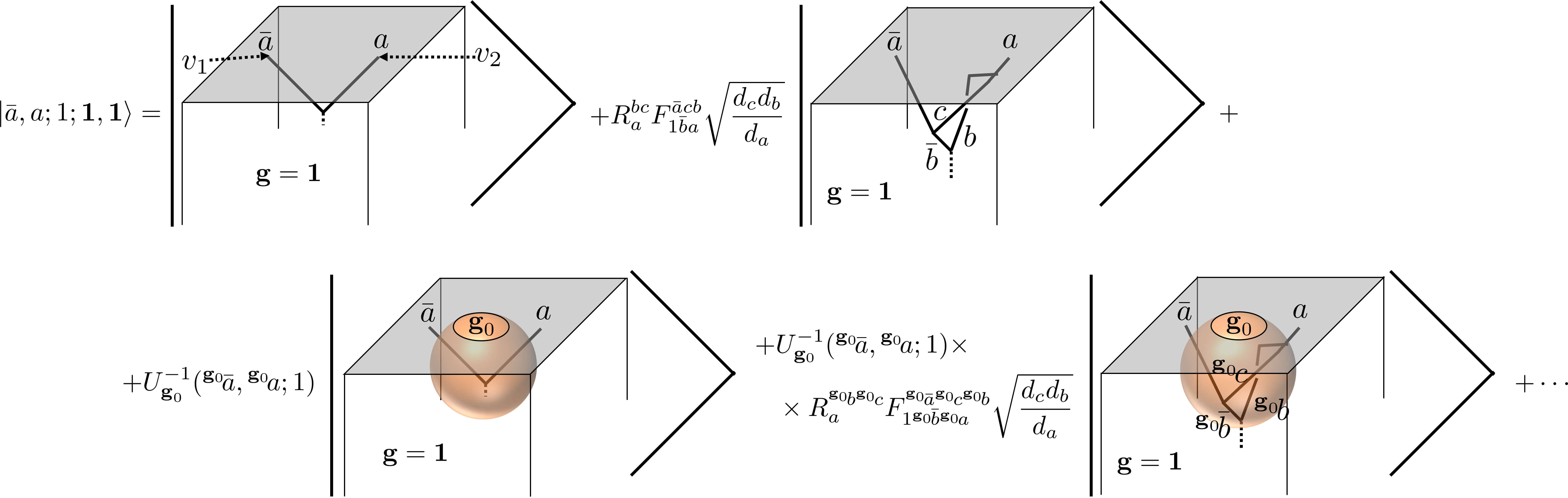
We also want to demand that away from the endpoints of the string. We therefore must superpose over domain wall configurations, and the relative amplitude between the state with and without a given domain wall is related by nucleating and expanding the domain wall in the graphical calculus. Some examples are given in the last two terms of Fig. 17. Importantly, since projects onto , where is the degree of freedom on cube , only contains states where the cubes and contain identity group elements.
VIII.2.3 The surface realizes
Next we want to check that the and symbols describing the algebraic properties of the deconfined surface anyons coincide with those of the UMTC that was used to define the model. Here we discuss explicitly; the argument for is essentially identical.
We begin by defining an operator graphically: it creates a particular braided fusion diagram far above the surface, slides it through the surface domain walls, and fuses it into the bulk braided fusion diagram. We choose the braided fusion diagram where fuse to , and fuse to , and finally fuses with to vacuum. This process is shown in Fig. 18a. The matrix elements between an initial configuration and is given by performing the appropriate graphical calculus in with symmetry fractionalization. We may then suggestively name a state
| (160) |
where we are ignoring all of the local degrees of freedom near the endpoints of the strings involved. Similarly, we can graphically define a different operator by fusing in a different braided fusion diagram; this diagram has and fusing to , and fusing to , then and fusing to vacuum. This is shown in Fig. 18b. We can then define a state
| (161) |


Consistency of the graphical calculus demands that
| (162) |
because we may always evaluate the fusion diagrams involved in calculating matrix elements of by performing an -move first. Therefore the states obey
| (163) |
which justifies the names we have given the states; the point-like excitations which we have called indeed obey the -moves given by . A precisely analogous argument holds for -symbols; therefore the surface topological order is indeed given by .
We also note that projectors onto fixed anyon sectors inside a loop can be defined graphically. In , such a projector is given by
| (164) |
where is a Wilson loop operator (specifically a closed string operator) for on the loop . We define graphically by taking this same superposition of Wilson loops and fusing them onto the surface (again passing through domain walls as necessary). It is clear from consistency of the graphical calculus that this definition will also justify our labelings of states; by choosing different , we can measure the fusion channels associated with different sets of anyons to be as we have claimed.
VIII.3 Surface symmetry fractionalization
Here we analyze the symmetry action on the surface topological order. Remarkably, we will see that the symmetry localization ansatz of Eq. (34) is realized exactly, along with the symmetry fractionalization relation of Eq. (35). Moreover, we also demonstrate how the symmetry fractionalization pattern on the surface is described by the same choice of that was used to define the model.
VIII.3.1 Local degeneracy at anyons
First we note that each anyon at the surface carries a local degeneracy of states. As we will see, this degeneracy is local in the sense that local operators in the vicinity of the anyon can distinguish the different states.
The origin of this degeneracy lies in the fact that the cube operators are by definition zero whenever the vertices contained in the cube have violations of the vertex operator . The string operator described in the previous section breaks the fusion rules at , that is, acting on the ground state it makes a state with . If contains the vertex , then we have
| (165) |
This is why the state only contains states where the group label in the cubes and , at the endpoints of the string, is the identity.
Next, let us define an operator , which is given by , but with the phase factors of involving the vertex removed. For example, if there was an anyon at the vertex where , and meet in Fig. 13a, then would be defined by Eq. (148) with the factor removed.
It is clear by inspection that commutes with all for any vertex , cube , and plaquette which does not contain . Recalling that, for containing , on any state with , this means that
| (166) |
because .
The model therefore has some degeneracy, but since is local, the degeneracy is non-topological. Of course, cannot change the net anyon type in cube . Therefore, there are many eigenstates, related by local operators, which have the same anyon types at . We label these states . The labeling scheme is as follows: means that the (physical) anyons and are present on the surface, the means that and are in the fusion channel, and the labels mean that and , where are the group elements on . We fix a gauge by defining
| (167) |
where was gauge-fixed earlier. The state is illustrated pictorially in Fig. 20a.
Accordingly, we can define the string operators by
| (168) |
where is specified by Eq. (158). This implies that
| (169) |


It is straightforward to check that the wave function of is obtained in the same way as that of in Fig. 17, but starting from a reference state where the anyons are surrounded by domain walls, as in Fig. 19a. There is a subtlety here that the reference state should not have phase 1; instead, as shown in Fig. 19b and more schematically in Fig. 19c, moving a string through the domain walls picks up a phase of . This changes the wavefunction by a global phase and thus is simply a basis choice, but it does arise from our definitions of the string operators in Eq. (168).
Importantly, the physical anyon type cannot be changed by a local operator such as . However, since still acts on the anyon labels on the links in , the anyon label along the string that ends at changes to . Therefore, if in the wave function a string type labeled ends at , then the physical anyon type at is , where is the state of the degree of freedom in cube .
Note that the local degenerate state space at each anyon excitation on the surface forms a regular representation of . In general such a representation is reducible, which means that the Hamiltonian should admit symmetry-preserving perturbations that lifts this degeneracy. The understanding of the ground and excited states, and in particular the symmetry fractionalization analysis below, would then have to be modified, but the data that characterizes symmetry fractionalization should remain unchanged, up to possible gauge transformations.
VIII.3.2 Symmetry localization
For simplicity, we consider only simple states with two anyons and fusing to the identity; the generalization is straightforward.
We define the topological symmetry transformation
| (170) |
Obviously this map by definition obeys Eq. (28) with the original that we input into the Hamiltonian. To show that we have the correct symmetry fractionalization pattern at the surface, we first need to show that the global symmetry action acts in a way according to Eq. (34), which we refer to as symmetry localization. Subsequently we must show that Eq. (35) is obeyed with defined in Eq. (170) and with given by the that we input into the Hamiltonian.


We compute by examining the wavefunction. Consider in particular the terms shown in Fig. 20a, where all of the group elements except for are either or . By our normalization and gauge fixing, the first term has amplitude . By nucleating a domain wall of type , as in the second term in Fig. 20a, and expanding it, we eventually reach the third term, picking up various s and s as the domain wall expands.
Now apply the symmetry operator to , which right-multiplies all group elements by but does not change any link labels. The result is shown in Fig. 20b.
Separately, we may compute the wavefunction for the state ; this is shown in Fig. 20c. Comparing Figs. 20b and 20c term-by-term and using the consistency conditions for and , we find that
| (171) | ||||
| (172) |
where we have defined the local operators as they act on a state with anyon at by
| (173) |
where labels the degree of freedom on the cube containing the vertex .
The topological part of the symmetry action that was previously defined has indeed appeared in the actual global symmetry action of the model, and the remaining factors decompose into local factors , as expected.
VIII.3.3 Symmetry fractionalization
Verifying Eq. (34) is now a matter of straightforward computation. Using Eq. (37):
| (174) | ||||
| (175) | ||||
| (176) |
This demonstrates that the symmetry fractionalization at the surface is, as we have claimed, given by the and which were put into the theory.
As a technical aside, our definition of is not invariant under independent basis rotations of the local degrees of freedom in different anyon sectors. For a simple example, we could modify the states with a - or -dependent phase. Such basis changes yield surface fractionalization with data that is gauge-equivalent but not identical to a given choice of and that defines the model.
VIII.3.4 Anti-unitary symmetries
All of the prior analysis can be repeated for anti-unitary symmetries. We define the analog of Eq. (170)
| (177) |
Following the same argument, the anti-unitary operator
| (178) |
localizes according to Eq. (172), with the local operators still defined by Eq. (173). Note that the physical surface anyon states do not involve any domain data since the microscopic domains fluctuate. However, the Hilbert space configurations naturally carry domain information. This means that when repeating the calculation, the graphical calculus involves the data defined in Sec. IV, and the domain labels must be carefully tracked. The amplitudes in the anti-unitary version of Fig. 20 are thus expressed in terms of the data with tildes, but using -equivariance, they can be converted to the physical and data via Eqs. (86)-(89).
IX Generalizations: spatial symmetries, continuous, infinite
So far we have defined models that possess an internal, on-site symmetry action, which may be unitary or anti-unitary. Furthermore, the state sums defined in the previous sections require finite, discrete groups. Here we briefly discuss the generalizations of the construction to spatial (crystalline) symmetries, and to continuous and/or infinite symmetry groups.
IX.1 Infinite and/or continuous
When is compact and continuous (and for simplicity of this discussion connected), there is a natural generalization of our state sum obtained by replacing the sum over group element labels by integrals, , where is the volume of and is the number of 0-simplices. The integration measure is then taken to be the Haar measure on . We note that such a construction necessarily still defines a SPT due to the translation invariance of the measure. Therefore our construction yields topologically invariant path integrals on non-trivial flat bundles for continuous as well. Our Hamiltonian construction furthermore also goes through straightforwardly as well.
For infinite discrete we can define the state sum as a limit of a sequence of finite discrete groups that approach in the limit. However, if our conjecture in Sec. III is true, then the above modifications are actually all unnecessary, and our construction naturally gives a concrete way to compute the path integral on any flat bundle regardless of whether is infinite, continuous, or compact.
We note that our discussion of obtaining cohomology invariants in Sec. V.1 applies only to finite groups; therefore some other method would be required to find cohomology invariants for the case of infinite or continuous .
IX.2 Spatial symmetries
Given a symmetry group , it is possible that certain elements of are spatial symmetries, meaning that they act on the quantum system by some combination of translations, rotations, and reflections in space. Here we briefly discuss some issues in incorporating such symmetries into our discussion. There are three aspects to the discussion, which we will briefly address:
- 1.
Classification of spatial symmetry fractionalization and anomaly computations
- 2.
Path integral construction
- 3.
Hamiltonian construction: boundary and bulk symmetries
IX.2.1 Classification of spatial symmetry fractionalization and anomaly computations
First, let us consider classification of symmetry fractionalization and anomaly computations. It is expected that the classification of symmetry-enriched topological phases with spatial symmetries is identical to the case with internal symmetries, where spatial parity reversing symmetries are treated as anti-unitary symmetries. This expectation has already received strong direct supporting evidence from studies of SPT statesSong et al. 2017; Huang et al. 2017; Thorngren and Else 2018 and from the understanding of the relation between Lieb-Schulz-Mattis theorems and mixed anomalies between translation and on-site symmetries.Cheng et al. 2016 Therefore, the same data that characterizes symmetry fractionalization and the same anomaly calculations are expected to hold even in the case of spatial symmetries.
The general reason for this expectation is as follows. The low energy universal properties of these SET states is described by a TQFT enriched with a symmetry. The TQFT always has a diffeomorphism symmetry, which in particular includes the isometries of space. Any spatial symmetry of the microscopic Hamiltonian can then be taken to correspond to a combination of an internal symmetry in the field theory together with an isometry of the space. Stated differently, one can consider a combination of the spatial symmetry of the microscopic Hamiltonian, followed by an isometry of space in the field theory, which then leads to an internal symmetry acting in the field theory. Examples where the above logic is borne out are prevalent throughout the literature regarding effective quantum field theories describing quantum many-body systems. Thus classifying different ways of incorporating internal symmetry in a TQFT should also give the classification of spatial symmetry enriched topological phases of matter.
IX.2.2 Path integral construction
The state sum for the path integral proceeds by choosing a triangulation and a branching structure. Therefore we can consider triangulations and branching structures that are invariant under a space-time symmetry of interest. For example, one can consider a space-time manifold , and one can consider a triangulation and branching structure that reduces on to a particular (finite) space group symmetry of interest. In this case, the amplitudes that are summed over in the path integral possess a symmetry. If we pick such that , then we can consider the diagonal group elements of the form , where . Then we can consider any type of space group symmetry fractionalization, and the path integral will possess the space group symmetry.
Alternatively, one can consider a 4-manifold with boundary such that has a triangulation and branching structure associated with the space group symmetry of interest. We can take the triangulation of to correspond to just adding a single “bulk” 0-simplex to which all 0-simplices in the triangulation of are connected. The resulting wave function will be symmetric under , and again as in the previous paragraph we can consider the diagonal action for .
Therefore, the path integral construction can be easily extended to space group symmetries for which there is a triangulation and branching structure that preserves the space group symmetry. It is an interesting question whether a symmetric triangulation and branching structure exists for any given space group symmetry.
IX.2.3 Hamiltonian construction
Our Hamiltonian construction in general picks a preferred direction to correspond to an “arrow of time” in evaluating the braided fusion diagrams. As such, our Hamiltonian construction, while it preserves lattice translational symmetries, in general breaks point group symmetries. It is a non-trivial question whether our general construction can be modified to allow space group symmetries in general.
It may be possible to consider certain classes of UMTCs that are invariant under changing the “time” direction. This seems to be a generalization of the “tetrahedral” symmetry of fusion categories to a higher dimensional version, which we may term “hypertetrahedral” symmetry. UMTCs that possess such a symmetry and which have self-dual anyons will then give Hamiltonians that are independent of the chosen “time” direction and any orientations on the edges. While the trivalently resolved cubic lattice is still incompatible with point group symmetries, we expect it is possible to consider Hamiltonians on other trivalent lattices, or to use certain gadgets that allow for sites with more than three edges, that would be compatible with any given space group symmetry.
IX.2.4 Spatial reflection symmetries mapping to anti-unitary internal symmetries
Here we consider spatial reflection symmetries in the path integral construction and demonstrate how they can be captured using the anti-unitary on-site action. We leave for future work to study spatial reflection symmetry in the Hamiltonian formalism, and in particular to understand spatial reflection symmetry fractionalization in the (2+1)D surface SET in the Hamiltonian construction.
Accordingly, suppose that contains symmetries that reverse spatial parity. For simplicity, we choose to examine a pure reflection , but the following discussion holds for any unitary parity-reversing element of . Since acts unitarily on the wavefunction but changes the locations of vertices, the desired -action on the wavefunction is a modification of Eq. (63):
| (179) |
where, as a reminder, the are the degrees of freedom on , and label boundary vertices. The notation means the image under spatial reflection of the vertex .
This is not enough to determine the consistency equations for the objects that appear in the state-sum. In order to do so, we need to understand the way that group multiplication by acts onsite. We claim that
| (180) |
where there is no group multiplication. To see this, note that under the action of reflection, every 4-simplex changes its orientation. If the data associated to the 4-simplex remains unchanged, this orientation reversal simply complex conjugates the corresponding amplitude . Eq. (180) therefore follows. Combining Eq. (180) and (179), we find
| (181) |
This is exactly the same as Eq. (81); that is, the onsite action of a parity-reversing symmetry should be anti-unitary, despite the fact that the global action is unitary. The rest of the derivation following Eq. (81) therefore holds for parity-reversing symmetries as well, provided the definition Eq. (II.2) of is reinterpreted to refer to the (anti-)unitarity of the onsite action of . In particular, we should be choosing anti-unitary despite the unitarity of the overall symmetry action.
Repeating the above argument for which is both anti-unitary and spatial parity-reversing, we find that should have a unitary onsite action as in Eq. (63).
X Discussion
We have shown how the symmetry fractionalization data determines a (3+1)D SPT, and thus determines an element . As we have discussed, it is also known that there is an obstruction in defining a -crossed braided tensor category from a given symmetry fractionalization class. In mathematical terms, there is an obstruction in lifting a categorical action to a -crossed braided tensor category. It is clear on physical grounds that , since we physically understand the presence of a non-trivial bulk (3+1)D SPT as an obstruction to defining a consistent theory of symmetry defects purely at the (2+1)D surface. On mathematical grounds, we expect that the categorical action defines a single element of , not two distinct elements. Nevertheless, to have a complete mathematically rigorous theory, we must prove that , which we leave for future work.
While we have given a concrete general method to compute the anomaly, there are still many interesting and important directions left for further study. For example, it would be interesting to understand “anomaly in-flow” in these models. That is, to understand precisely how processes on the surface give rise to inconsistencies that are canceled by the bulk SPT. Along these same lines, it would be interesting to understand how to extract a 4-cocyle through consideration of certain processes in the (2+1)D surface theory in a way which would not require a complete computation of the path integral on closed 4-manifolds with non-trivial -bundles.
A related issue is to make contact between the results here and the relative anomaly formula derived in Ref. Barkeshli and Cheng 2020. It was conjectured in Ref. Barkeshli and Cheng 2020 that the relative anomaly obtained there could be canceled by a bulk (3+1)D SPT. The bulk construction provided here should in principle provide a way of demonstrating this explicitly, however we have not pursued this direction here.
As noted in the main text, while our state sum requires a sum over group elements, we conjecture that every term in the sum over group elements is identical, and therefore that the sum over group elements is actually not required. The action would therefore enter only through the presence of non-trivial holonomies along non-contractible cycles of the space-time manifold. It would be useful for practical computations to prove this rigorously.
While we have presented our construction in terms of an explicit state sum associated with a triangulation of the space-time manifold, we expect that there should be an alternative formulation where the path integral on arbitrary space-time manifolds and bundles can be obtained by gluing together path integrals on simpler manifolds via a handle decomposition. Such a formulation was developed for the Crane-Yetter state sum (i.e. the case where is trivial) in Ref. Walker 2006. The extension to non-trivial would require, for example, defining a vector space for 3-manifolds equipped with bundles via skein modules on bundles. A simple version of such a formulation for the case of space-time reflection symmetry was used in Ref. Barkeshli et al. 2019b for computing path integrals on non-orientable manifolds. Such constructions could lead to more efficient ways of computing anomaly indicators, and we leave them for future work.
It is clear that similar ideas should hold in all dimensions. Symmetry fractionalization in general dimensional TQFTs with symmetry should define a -category where the objects (0-morphisms) correspond to group elements of , and there is a action on the -category. This -category should then define a -dimensional state sum for a -SPT, which then can be used to compute the anomaly. We note that initial steps for computing anomalies in (3+1)D by defining a (4+1)D path integral have already been taken in some simple cases.Kobayashi and Shiozaki 2019
Finally, we note that our Hamiltonian constructions explicitly break most spatial symmetries. It would be interesting to develop constructions that preserve any given spatial symmetry. However we note that even the simpler Levin-Wen models for (2+1)D topological orders (and Walker-Wang models for (3+1)D topological orders) have not been generalized to take as input arbitrary unitary (braided) fusion categories in a way that is compatible with point group symmetries on the lattice.
Acknowledgements.
MB thanks Parsa Bonderson, Meng Cheng, Chao-Ming Jian, Kevin Walker, and Zhenghan Wang for previous collaborations and ongoing discussions. MB also thanks Shawn Cui for helpful conversations. This work is supported by NSF CAREER (DMR- 1753240), Alfred P. Sloan Research Fellowship, and JQI- PFC-UMD.Appendix A Invariance properties of state sum
A.1 Invariance under Pachner moves
In this appendix, we demonstrate that our path integral is invariant under the 3-3 Pachner move. Other Pachner moves are treated similarly, but the diagrammatics are considerably more involved. Our treatment is essentially identical to that of Ref. Cui 2019; we reproduce the calculation here to (a) convert the calculation to our conventions and (b) make our paper self-contained.
Before doing this, we prove two “merging lemmas” stated in Ref. Cui 2019. The first is the equality of the far left- and far right-hand sides of Fig. 21a, where the intermediate equalities are the proof of the merging lemma. The first two equalities follow from the usual UMTC diagrammatic equation
| (182) |
where we have been implicitly assuming for all . Conservation of total anyon charge means that in the third diagram, the only nonzero term occurs when is the identity, producing the last equality.
We then use this first merging lemma to prove a second, shown in Fig. 21b.


With these lemmas in hand, we can prove invariance under the 3-3 Pachner move. Given five vertices , a 3-3 Pachner move takes the 4-simplices , all positively oriented, to the 4-simplices , also all positively oriented. In doing so, the 2-simplex is replaced by the 2-simplex and the 3-simplices are replaced by the 3-simplices . Our aim is to show that
| (183) |
with fixed labels on all other simplices involved.
We first contract all of the domain walls in the diagrams and examine the symmetry fractionalization factors that arise. These are given by the factors of and in Eq. (44). On the left-hand-side (LHS) of Eq. (183), we obtain
| (184) |

Our aim will be to use the merging lemmas in Fig. 21 to perform the sums on and in Eq. (183). In order to do so, both diagrams should involve, say, , but as naturally written, the diagram for involves and the diagram for involves . Hence, we sweep a domain wall through the diagram for as shown in Fig. 22. By the consistency of the graphical calculus, we may evaluate the diagram either before or after this sweeping process; as long as we account for all of the factors of or which arise in the sweeping process, the value of the diagram is unchanged. At the algebraic level, this process simply transforms all of the - and -symbols in the explicit formula Eq. (44) for by using the consistency condition Eq. (29). The proportionality factor in Fig. 22 is given by
| (185) |
After this transformation, the symmetry factors for the LHS of Eq. (183) are times the factors in Eq. (184).
The symmetry factors for the right-hand side (RHS) of Eq. (183) are
| (186) |
Laborious but straightforward use of the consistency conditions Eqs. (36) and (37) demonstrates that the symmetry factors on the LHS and the RHS are now equal.
Canceling these symmetry factors reduces each side of Eq. (183) to of a product of three diagrams with no domain walls or symmetry factors. We define
| (187) | ||||
| (188) |
where do not involve quantum dimensions of any of the summands in Eq. (183). We can now do graphical calculus to demonstrate the equality of those products of diagrams, as shown in Figs. 23 and 24. Careful examination of the final diagrams shows that both the diagrams and normalization factors are indeed equal, proving Eq. (183).


A.2 Independence of fusion channel on 3-simplices
In defining our path integral, we made an arbitrary choice of fusion channel for the data on the 3-simplices. Suppose we change the fusion channel; we wish to show that the path integral is unchanged. On a closed manifold, each 3-simplex appears in exactly two 4-simplices with opposite induced orientation. For concreteness we focus on the 3-simplex which, again for concreteness, we suppose is in the 4-simplices (+ orientation) and (- orientation). We define the unitary basis transformation
| (189) |
One can check that
| (190) |
where is the usual -symbol, although this form does not make the unitarity of manifest. It can also be checked that
| (191) |
We can relate amplitudes in the original fusion channel to amplitudes in the new fusion channel by an -move:
| (192) | ||||
| (193) | ||||
| (194) |
where the second line follows from the unitarity of the -symbols and in the third line we relabeled . We have explicitly labeled the relevant 3-cell as it appears in each amplitude . This equation is shown graphically in Fig. 25.

The right-hand side is precisely the amplitude which would appear if we had chosen to construct the path integral using the new fusion basis for the 3-simplex . Therefore the choice of fusion channel does not affect the partition function for a closed manifold. The same is true for an open manifold if the 3-simplex is not on the surface. If the 3-simplex is on the surface, then there is no cancellation; instead the amplitude in the wavefunction of the initial configuration is related to the amplitude of the final configuration by an -symbol, which is as expected.
A.3 Independence of deformation of 3-simplex data
We also chose a particular deformation of the data on the 3-simplices towards 0-simplices, as in Fig. 2(c). Suppose that instead of deforming a -simplex, call it , towards , we deformed it towards instead, where or . Our claim is that the term in the state sum with data on in the original deformation is equal to the term in the state sum with on in the new deformation. The reason is as follows. For each 4-simplex containing the amplitude corresponding to in the new deformation can be related to the amplitude in the original deformation by sliding anyon lines through domain walls as shown in Fig. 26. The labeling of could be for , or for , etc. Doing the graphical calculus, shown in Fig. 26 for the case with positive orientation and checked similarly for the other cases, leads to (for all possible )
| (195) |

Here is the relative orientation of to the 4-simplex . If the 3-simplex is in the bulk of the spacetime manifold, then appears in exactly two 4-simplices and , one with each relative orientation. Hence, for every term in the state sum, the above factors coming from and cancel out, and the state sum is unchanged. If is on the surface, then the aforementioned phase factor is the relative amplitude in the wavefunction between two states where the braided fusion diagrams labeling the state differ by sliding the appropriate domain walls over anyon lines, which is as we expect.
A.4 Independence of deformation of 2-simplex data
Another choice was a deformation of the 2-simplex data towards a 0-simplex. Consider a -simplex . For simplicity of presentation we assume there are no vertices such that the branching structure orders or ; this assumption may be relaxed at the cost of checking a few extra cases in what follows. Suppose that we deformed towards for or instead of towards . We relate the term in the newly deformed state sum with on the simplex in question to the term in the old deformation with .
Let us examine each 4-simplex which contains , where enumerates all such 4-simplices. There are three possibilities for ; without loss of generality, can be labeled or , where all that matters is whether the additional vertices are smaller than 2 or larger than 4. For each of these three cases one can determine the ratio of the amplitudes and with the old and new deformations, respectively. The portions of the diagrams which differ for each of these cases are shown in Fig. 27. Graphical calculus shows
| (196) |

Of course, the 4-simplex always contains exactly two 3-simplices which involve , where enumerates the two 3-simplices. Each 3-simplex is labeled either or for some . Define
| (197) |
Then we see that Eq. (196) can be rewritten
| (198) |
where the product is over all 3-simplices in containing and is the orientation of induced by . But every bulk 3-simplex appears in exactly two 4-simplices with opposite induced orientations. Since depends only on the 3-simplex labels, it is now clear that the bulk factors of all cancel pairwise, that is, for a closed manifold,
| (199) |
Therefore, the two terms in question in the state sum are equal, as desired.
A.5 Independence of branching structure
In Ref. Cui 2019, Cui proves the invariance of a closely related TQFT under changes of branching structure. The proof constructs, for each configuration in the state-sum with the original branching structure, a corresponding configuration in the state-sum with the new branching structure, then shows that the amplitude associated to that configuration is the same with both branching structures. The construction and proof are rather involved, but apply mutatis mutandis to our state-sum. We therefore do not reproduce the proof here.
A.6 Gauge invariance under vertex basis gauge transformations
Consider a basis transformation on the fusion or splitting spaces given by a unitary map . Our claim is that on a closed manifold , the path integral is invariant under this basis transformation. On a closed manifold, each 3-simplex appears twice, once with positive orientation and once with negative orientation. Hence, for a fixed term in the state sum, each fusion vertex (say, the fusion vertex associated to a positively oriented 3-simplex) will appear exactly once and its dual splitting vertex (say, the splitting vertex associated to the same 3-simplex with opposite orientation) will also appear exactly once. Let be the path integral amplitude with fixed anyon and group data, but we place the splitting vertex in the state and the fusion vertex in the state . The gauge-transformed path integral involves sums over the terms with , so we compute that sum:
| (200) | ||||
| (201) | ||||
| (202) |
where the prime indicates the gauge-transformed amplitude. The final expression is exactly the same amplitude in the original gauge, which demonstrates the desired equality.
On an open manifold, these gauge transformations on bulk 3-simplices cancel in the same way. The gauge transformations do not cancel on surface 3-simplices, but instead transform the wavefunction in the expected way.
In the presence of anti-unitary symmetries, the gauge transformation rule needs to account for the group elements; the gauge transformation takes the form
| (203) |
where the hat refers to the gauge-transformed state and the fusion vertex is in domain . Demanding -equivariance of the gauge transformations, we find
| (204) |
where the last equality defines the shorthand . Using this object, the above argument for gauge invariance of the path integral goes through exactly on an orientable manifold.

On an unorientable manifold, in order to define the path integral, as described in Sec. IV, we should cut open the manifold to obtain an orientable open manifold. For any 3-simplex which does not lie entirely on the cut, the argument goes through as above. However, on the cut, we identify the data on two 3-simplices with the same relative orientation. The key difference is that the group elements on the vertices of those two 3-simplices are twisted by an anti-unitary group element . That is, if is a 3-simplex lying on the cut and has positive induced orientation, then appears in two diagrams in the path integral shown in Fig. 28. These two diagrams pick up the gauge transformation
| (205) |
where we have used the fact that . Hence the path integral remains gauge-invariant. The fact that the boundary conditions for the group elements are twisted by a group element with an anti-unitary action is what ensures that the path integral is gauge-invariant on an unorientable manifold.
A.7 Gauge invariance under symmetry action gauge transformations
Gauge transforming the symmetry action changes the way that the global symmetry action factorizes into its topological and local parts according to Eq. (34). Given an anyon diagram with domain walls, the gauge transformation changes the diagram by a phase for every crossing of a domain wall of type with an anyon as shown in Fig. 29a, where checks over diagrams represent the gauge-transformed diagram. We presently check that our state-sum is invariant under this transformation.


It is straightforward to check by inspecting Fig. 4 that the amplitudes for a 4-simplex, each crossing of a domain wall over an anyon line in the full diagram can be associated to a 3-simplex, i.e. the set of crossings on the left-hand-side of Fig. 4 is in correspondence with the crossings on the right-hand-side. Using the diagrammatic rules in Fig. 29a, we see that the crossing in a 3-simplex (here label vertices) appearing in a 4-simplex picks up a factor of under gauge transformations, where is the orientation of induced by the 4-simplex . Since, on a closed manifold , each 3-simplex appears in two 4-simplices, each leading to opposite induced orientation, the factors of all cancel out in computing a single term of the path integral on . Hence the path integral on a closed manifold is gauge invariant.
On a manifold with boundary, the gauge transformations of crossings associated to bulk 3-simplices still cancel out. However, gauge transformations of crossings involved in surface 3-simplices do not cancel. Instead, they modify the wave function by changing the value of the wave function to match the gauge-transformed value of the closed anyon diagram on the boundary of , as expected.
In the presence of anti-unitary symmetries, we should modify the gauge transformation rules Fig. 29a to those in Fig. 29b, which allows us to define the shorthand objects by the equation
| (206) |
With this definition, the only difference is that the crossings in a 3-simplex pick up the gauge transformation factor . On an orientable manifold, the above argument carries through straightforwardly.
On an unorientable manifold, we consider the same setup discussed in the previous section on vertex gauge transformations. For 3-simplices which do not lie entirely on the cut, the argument for the unitary case goes through, mutatis mutandis. For a 3-simplex on the cut, its two appearances are, as before, shown in the diagrams in Fig. 28. These two diagrams pick up the gauge transformation factors and respectively, where is some anti-unitary group element. But , hence
| (207) |
Hence the path integral is gauge-invariant, even on an unorientable manifold. As for the vertex transformations, this gauge invariance fundamentally requires that the boundary conditions for the group elements are twisted by a group element with an anti-unitary action.
A.8 Mirroring 3-simplices about the vertical axis
Our path integral is built by assigning a fusion diagram to the 3-simplex , corresponding to the process . Mathematically this corresponds to an element of (or, in the category theory terminology, this corresponds to an element of the Hom space Hom). Given an orientation of the 3-simplex, the 2-simplices and have the same induced orientation, which is why and both appear in the domain (or codomain, for the opposite orientation of the 3-simplex) of this process. However, it is not a priori clear why we should not mirror the entire diagram about the vertical axis when constructing the amplitudes associated to 4-simplices; that is, use Hom instead.
We claim that on a closed manifold, the path integral is invariant under this mirroring, provided that the over/under-crossing in the diagram is also changed. That is, constructing using the diagram in Fig. 30(a) yields the same path integral as in Fig. 30(b), and likewise Figs. 30(c) and (d) would yield the same path integral on a closed manifold.
Note that mirroring the diagram about the vertical axis and changing the over- to under- crossing is equivalent to rotating the entire diagram about the vertical axis by . Thus another way of stating the result is that the path integral is invariant under rotating the diagrams associated with all 4-simplices by around the vertical axis.

The idea of the proof is the following. Start with Fig. 30(a) and shrink the domain walls, evaluating the symmetry factors as appropriate. Next, slide all of the 3-simplex lines into their positions in Fig. 30(b). This introduces many twists into the diagram. Then, remove those twists with -moves. Finally, reintroduce the domain walls as appropriate; this produces, after some isotopy, Fig. 30(b). The whole process introduces a factor of for each fusion space and a factor of for each splitting space in the diagram (use of the consistency of and moves is required for the vertex inside the domain walls). Since each 3-simplex appears once with each orientation in a closed manifold, each vertex appears once as a fusion vertex and once as a splitting vertex. Hence the -moves cancel.
On a non-orientable manifold, we consider, as usual, cutting the manifold to produce an orientable one. For all 3-simplices away from the cut, the above argument works identically. The only difference is for 3-simplices on the cut, which appear once on each side of the cut with the same induced orientation. However, there is a twist of the group elements on both sides of the cut; the 3-simplex lives in domain on one side and on the other side, where . Hence we pick up , which still cancels out by the -equivariance of the -symbols.
A.9 Changing over-crossing to under-crossing
In this section, we discuss changing the crossing in the diagrams defining our state-sum (Fig. 4) from an over-crossing to an under-crossing.
This crossing is the source of the factor of in the explicit formulas Eqs. (44) and (45), and it is easy to check that changing the crossing replaces by . By inspection of the consistency conditions for BTCs and symmetry fractionalization, if the data defines a consistent BTC with symmetry fractionalization, then the data also defines a consistent BTC with symmetry fractionalization. Therefore, changing the crossing interchanges the path integrals for these two theories.
The modular and matrices, where is a diagonal matrix with
| (208) |
clearly obey , where belong to the BTC .
It immediately follows that, on a closed manifold, the Crane-Yetter invariant for and are complex conjugates. This is because for a UMTC ,
| (209) |
for the Crane-Yetter invariant. Here is the signature of the closed 4-manifold and is the chiral central charge given by
| (210) |
For our state sum with the symmetry action, it is less clear to see directly from the path integral what happens when we replace with and thus effectively interchange with . We will prove (subject to a mild additional assumption) that when the input to our state sum is a UMTC, this interchange complex conjugates our path integral. The technique is indirect, using the relative anomaly formalism of Ref. Barkeshli and Cheng 2020, but the result is borne out in the examples that we study in Sec. VI and also the example of with the unique rank 3 Abelian UMTC with fusion rules.
The method of proof is to show that, given two fractionalization classes given by data and , the path integral on any closed -manifold (with a general background gauge field) obeys
| (211) |
Rephrased in terms of anomalies, we wish to show that the anomaly of relative to is the inverse of the anomaly of relative to . Under the additional assumption that some non-anomalous class exists for any , setting to the non-anomalous class proves the desired equality, since on any manifold a non-anomalous SPT has .
In general, different fractionalization classes form an torsorBarkeshli et al. 2019a, where is the set of Abelian anyons in the theory. That is, given any two fractionalization classes for , there exists such that
| (212) |
where is the double braid defined in Eq. (15). The anomaly of relative to isBarkeshli and Cheng 2020
| (213) |
In what follows, the factors of and will be unchanged throughout, so we suppress all of their arguments.
We now reinterpret as a relative anomaly between theories with the -symbol . Since is Abelian, we have
| (214) |
Therefore, according to Eq. (212),
| (215) |
Setting and substituting into Eq. (213), we obtain
| (216) |
Comparing this expression to Eq. (213), we directly see that we can interpret as the anomaly of relative to , where is obtained from using in Eq. (212) with the double braid computed with the -symbol . Explicitly,
| (217) | ||||
| (218) |
where the last equality follows from Eq. (215). Hence . Furthermore, since relative anomalies form an Abelian group, the anomaly of relative to is the inverse of the anomaly of relative to . Thus we have proven that , defined as the anomaly of relative to , is also the inverse of the anomaly of relative to , as claimed.
Appendix B Exhaustiveness of cohomology invariants
In Sec. V, we constructed sets of cohomology invariants for using the Smith normal form of a matrix version of the coboundary operator. In this appendix, we demonstrate that those invariants fully characterize the cohomology group. That is, following the notation in Sec. V
| (219) |
In the following, when no ambiguity results we will abuse terminology slightly by using “cochain” (and “cocycle”, etc.) to interchangably mean either a function or its “vectorized” form , where is a real-valued vector of length defined modulo integers.
Recall first that -cocycles are vectors which satisfy Eq. (102). Treating as a map between vector spaces over , it follows that all elements of are cocycles, but not all cocycles are in . However, all -coboundaries are in (modulo the integer ambiguity).
Next we claim that
| (220) |
To see this, note that by construction, is the matrix of the coboundary map for . (Note that is an unambiguously defined integer matrix, while vectors which represent cocycles over are only defined modulo integers.) Hence, generators of correspond to generators of . The latter, however, is known to be trivial for any finite group for ; that is, is trivial, which proves Eq. (220). One way to prove this latter fact is to use the universal coefficient theorem, which, for present purposes77 7 The universal coefficient theorem is usually stated as the existence of a split exact sequence, but the fact that all the groups involved are known to be Abelian means we can rewrite it in the form Eq. (221)., states thatHatcher 2002
| (221) |
where are the homology groups of , is the group of homomorphisms from to , and Ext is the Ext functor, whose detailed definition we do not need here. The important properties of Ext are that, for any finitely generated groups , and Abelian group ,Hatcher 2002
| (222) | ||||
| (223) | ||||
| (224) |
Using the fact that , it follows that . Further, homology groups for over are finiteBrown 1982, so by inspection is trivial. Thus , as claimed.
We now claim that if two cocycles have the same invariants as defined in Eq. 106, then they differ by an element of ; that is, they are in the same cohomology class. This is enough to prove equality in Eq. (219).
Let and be two cocycles (over ) with identical for all . Then for each with ,
| (225) |
where this equation defines . Since has an integer inverse,
| (226) |
Recalling that is ambiguous up to an integer vector, we can freely replace without changing the cocycle. We now claim that, as a strict equality (over the reals),
| (227) |
This is readily verified by computation of
| (228) | ||||
| (229) | ||||
| (230) | ||||
| (231) |
In the third line, we were free to extend the sum over because the summand is zero when anyway, and we substituted the definition of .
Hence . But we showed earlier that Hence the cocycles represented by and are in the same cohomology class. This means that our invariants distinguish all cohomology classes; that is,
| (232) |
Furthermore, as we demonstrated in Sec. V, for each possible set of values of the invariants in Eq. (106) (each of which is a -th root of unity), there exists a cocycle defined in Eq. (107) which realizes that set of values. Hence
| (233) |
Appendix C Cellulations of manifolds
In this appendix, we give a general procedure for cellulating , where is a manifold of arbitrary dimension with a known cellulation. We then apply this procedure to some particular cases of to obtain cellulations used elsewhere in the paper.
We start with the case where consists of disjoint -simplices. Start with a 0-simplex, i.e. a single vertex . Obviously a point times is just , which can be cellulated with a single 0-simplex and a single 1-simplex. For later purposes, imagine first adding a -simplex and a 1-simplex , then identifying , as shown in Fig. 31a.


Now cross a 1-simplex, labeled , with . As shown in Fig. 31b, for each of the original 0-simplices 0 and 1, we repeat the procedure for crossing a 0-simplex with ; add “primed” vertices and and 1-simplices and . Next, for the 1-simplex , add a new 1-simplex and two new 2-simplices ,. Finally, identify the “top” and “bottom” to make the , that is, identify , , and . Even after identification, it is convenient to keep tracking and separately (and and , etc.) in order to define the 2-simplices.
By looking at the 2-simplex crossed with , we see how this process continues. Start by repeating the 0-simplex process for each 0-simplex in the original 2-simplex. This adds the primed vertices , , and , along with the 1-simplices , , . Next repeat the 1-simplex process for each 1-simplex in the original 2-simplex. This adds the 1-simplices , , and . Then, for the 2-simplex, add two new 2-simplices and , and three 3-simplices , , and . Finally, identify everything that consists entirely of primes with its unprimed version,e.g. .
In general, then, given an original -simplex , crossing it with should be done as follows. First, for each -simplex in the original object, we add new -simplices and new -simplices to the cellulation. As above, the -simplices are constructed by “priming” some vertices starting from the highest-numbered ones, and the -simplices are constructed in the same way but including both the unprimed and primed vertices for the lowest-numbered primed vertex. This crosses the original simplex with the interval. Then compactify the interval into by identifying simplices with all primed vertices with their unprimed counterparts; this means that in total, for each -simplex in the original object, only new -simplices appear after compactification.
It is now straightforward to see that given a cellulation of a general -dimensional manifold , one obtains a cellulation of by performing the above process on every individual simplex in the cellulation. That is, for each , we find all of the -simplices in the original cellulation of and add new -simplices and new -simplices in the manner described above.
C.1 Dealing with identifications
We start with a very simple example of the above procedure: cellulating given a cellulation of . From this, we will see how to cellulate and in the process understand how to pass from a cellulation of a manifold to one of , where simplices of are identified with each other to produce . This will be particularly helpful for generating a cellulation of .
We start with the cellulation of shown in Fig. 33a, which consists of four -simplices , five -simplices , and two -simplices and . According to our procedure we start with and add one new 1-simplex for each original 0-simplex. These are the 1-simplices , , , . For , we add a 1-simplex for each of the original 1-simplices, i.e. . We then add 2-simplices . Finally, for we add the 2-simplices and the 3-simplices . Identifying primed and unprimed vertices as usual yields a cellulation of shown in Fig. 32.

One can, of course, obtain a cellulation of by identifying various objects on the boundary of the cellulation of . To take a more systematic approach we start by compacting into , that is, identifying , , and and ask how this affects the prior procedure.
The key point is that when two simplices in are identified, we should also identify their corresponding “child” simplices. For example, generated one new -simplex and two new 2-simplices and , while generated the 1-simplex and the 2-simplices and . Thus, identifying in means that we should identify , , and in . It is easy to check that, for each identification of the “parent” simplices in to produce , identifying “child” simplices in in this manner is exactly how one produces the natural cellulation of from the given cellulation of .
To summarize, suppose we start with a manifold such that a list of simplices of can be pairwise identified to produce . To obtain a cellulation of , first obtain a cellulation of in the normal way. In this process, a “parent” -simplex of produces “child” and simplices in the cellulation of . Given two parent -simplices which are identified in passing from to , then identify their corresponding child simplices as well. After this identification process, we have a cellulation of .


C.2
We start from the cellulation of given in Fig. 6. A list of all the simplices contained in it, with identifications, is given in Table 4.
| -simplices | -simplices | -simplices | -simplices | |||
|---|---|---|---|---|---|---|
Let be the -simplices in the above cellulation of . Then by following the above procedure we obtain a cellulation of consisting of the data given in Table 5.
| -simplices | -simplices | -simplices | -simplices | -simplices | ||||
|---|---|---|---|---|---|---|---|---|
| for (7) | for (8) | for (6) | ||||||
| for (7) | for (7) | for (8) | for (6) | |||||
| for (7) | for (8) | for (8) | for (6) | |||||
| for (8) | for (6) | for (6) | ||||||
| for (8) | for (6) | |||||||
| for (6) | ||||||||
| for (6) |
C.3
| -simplices | -simplices | -simplices | -simplices | |||
|---|---|---|---|---|---|---|
Note that we distinguish the “front” and “back” 2- and 3-simplices by the order in which the vertices appear, i.e. and contain the same vertices but are distinct 3-simplices. Letting be the set of -simplices in the above cellulation and applying the above procedure, we obtain a cellulation of with the data given in Table 7.
| -simplices | -simplices | -simplices | -simplices | -simplices | ||||
|---|---|---|---|---|---|---|---|---|
| for (4) | for (4) | for (2) | ||||||
| for (4) | for (4) | for (2) | ||||||
| for (4) | for (4) | for (4) | for (2) | |||||
| for (4) | for (4) | for (2) | for (2) | |||||
| for (4) | for (2) | |||||||
| for (2) | ||||||||
| for (2) |
C.4
A simple cellulation of consists of two -simplices of opposite orientation glued together on their boundaries. It contains:
| -simplices | -simplices | -simplices | -simplices | |||
|---|---|---|---|---|---|---|
Following the above procedure, we obtain a cellulation of with the simplices given in Table 9.
| -simplices | -simplices | -simplices | -simplices | -simplices | ||||
|---|---|---|---|---|---|---|---|---|
| (4) | for (6) | for (4) | (2) | |||||
| for (6) | for (6) | for (4) | (2) | |||||
| for (6) | for (4) | for (4) | (2) | |||||
| for (4) | (2) | (2) | ||||||
| for (4) | (2) | |||||||
| (2) | ||||||||
| (2) |
Appendix D Partition function on
In this section, we explicitly compute our partition function on and show that it is always 1 in the absence of a background flux using the cellulation of containing eight 4-simplices that was constructed in the previous Appendix.
We first decompose the state-sum in the following way:
| (234) |
Here means the sum on all 2-simplices and 3-simplices not appearing explicitly in Eq. (234). We have chosen to group the diagrams so that the sums over certain - and -simplices can be separated; i.e. the 2-simplex appears only in the 4-simplices , so the other diagrams factor out of that sum.
Consider first the sum involving . The symmetry factors (factors of and ) in each diagram are
| (235) | ||||
| (236) |
Clearly these factors cancel. In fact, since for any pair, the two diagrams involve exactly the same 2-simplices, the only way that the symmetry factors could fail to cancel is if involves different 3-simplices. In the 4-simplices and , the factor of acts on and , respectively in both the and the diagram. Therefore all of these symmetry factors cancel out. The only pair that we need to check is the pair, which has
| (237) | ||||
| (238) |
Because these two 4-simplices involve , which are not a priori equal, there is not obviously a cancellation. However, because of the absence of background flux, . Therefore, all of these symmetry factors are 1.
What we have shown is that, for any given term in the state-sum, the factors of and either cancel out or are equal to 1. At this stage, one can now check straightforwardly that each anyon always appears with the same symmetry action on it, that is, for example, always appears as . Reindexing the sum (e.g. ) and performing the (now-trivial) sum on , we obtain precisely the Crane-Yetter state-sum for on , which is known to be 1, that is,
| (239) |
as desired. One can explicitly compute the Crane-Yetter state-sum on ; this is most conveniently done using the decomposition in Eq. (234) and the merging lemma in Fig. 21b, but since the result is known, we do not reproduce the calculation here.
References
- Wen (2004) Xiao-Gang Wen, Quantum Field Theory of Many-Body Systems (Oxford Univ. Press, Oxford, 2004).
- Wang (2008) Zhenghan Wang, Topological Quantum Computation (American Mathematical Society, 2008).
- Nayak et al. (2008) Chetan Nayak, Steven H. Simon, Ady Stern, Michael Freedman, and Sankar Das Sarma, “Non-abelian anyons and topological quantum computation,” Rev. Mod. Phys. 80, 1083 (2008).
- Moore and Seiberg (1989) Gregory Moore and Nathan Seiberg, “Classical and quantum conformal field theory,” Comm. Math. Phys. 123, 177–254 (1989).
- Witten (1989) Edward Witten, “Quantum field theory and the Jones polynomial,” Comm. Math. Phys. 121, 351–399 (1989).
- Barkeshli et al. (2019a) Maissam Barkeshli, Parsa Bonderson, Meng Cheng, and Zhenghan Wang, “Symmetry fractionalization, defects, and gauging of topological phases,” Phys. Rev. B 100, 115147 (2019a), arXiv:1410.4540 .
- Etingof et al. (2009) Pavel Etingof, Dmitri Nikshych, and Victor Ostrik, “Fusion categories and homotopy theory,” (2009), arXiv:0909.3140 .
- Gaiotto et al. (2014) Davide Gaiotto, Anton Kapustin, Nathan Seiberg, and Brian Willett, “Generalized global symmetries,” (2014), arXiv:1412.5148 .
- Benini et al. (2019) Francesco Benini, Clay Córdova, and Po-Shen Hsin, “On 2-group global symmetries and their anomalies,” Journal of High Energy Physics 2019, 118 (2019).
- Kapustin and Thorngren (2014) Anton Kapustin and Ryan Thorngren, “Anomalies of discrete symmetries in various dimensions and group cohomology,” (2014), arXiv:1404.3230 .
- (11) Implicit in this statement is that the symmetry acts in an on-site manner; that is, that the symmetry action in a lattice model decomposes as a tensor product of unitaries acting on each lattice site independently. It is possible to realize anomalous boundary theories in the dimension of the boundary by considering a non-on-site action of the symmetry.Chen et al. 2013 The precise extension of the “on-site” requirement for space-time symmetries has not yet been formulated, but presumably the requirement is that the symmetry must correspond to an on-site transformation combined with a classical permutation of coordinates and possibly complex conjugation.
- Vishwanath and Senthil (2013) Ashvin Vishwanath and T. Senthil, “Physics of three-dimensional bosonic topological insulators: Surface-deconfined criticality and quantized magnetoelectric effect,” Phys. Rev. X 3, 011016 (2013).
- Wang and Senthil (2013) Chong Wang and T. Senthil, “Boson topological insulators: A window into highly entangled quantum phases,” Phys. Rev. B 87, 235122 (2013).
- Chen et al. (2015) Xie Chen, F. J. Burnell, Ashvin Vishwanath, and Lukasz Fidkowski, “Anomalous symmetry fractionalization and surface topological order,” Phys. Rev. X 5, 041013 (2015).
- Senthil (2015) T. Senthil, “Symmetry-protected topological phases of quantum matter,” Annual Review of Condensed Matter Physics 6, 299–324 (2015).
- Kapustin (2014a) Anton Kapustin, “Symmetry protected topological phases, anomalies, and cobordisms: Beyond group cohomology,” (2014a), arXiv:1403.1467 .
- Kapustin (2014b) Anton Kapustin, “Bosonic topological insulators and paramagnets: a view from cobordisms,” (2014b), arXiv:1404.6659 .
- Freed and Hopkins (2016) Daniel S. Freed and Michael J. Hopkins, (2016), arXiv:1604.06527 .
- Chen et al. (2013) Xie Chen, Zheng-Cheng Gu, Zheng-Xin Liu, and Xiao-Gang Wen, “Symmetry protected topological orders and the group cohomology of their symmetry group,” Phys. Rev. B 87, 155114 (2013).
- Dijkgraaf and Witten (1990) R. Dijkgraaf and E. Witten, “Topological gauge theories and group cohomology,” Comm. Math. Phys. 129, 393–429 (1990).
- Song et al. (2017) Hao Song, Sheng-Jie Huang, Liang Fu, and Michael Hermele, “Topological phases protected by point group symmetry,” Phys. Rev. X 7, 011020 (2017).
- Huang et al. (2017) Sheng-Jie Huang, Hao Song, Yi-Ping Huang, and Michael Hermele, “Building crystalline topological phases from lower-dimensional states,” Phys. Rev. B 96, 205106 (2017).
- Thorngren and Else (2018) Ryan Thorngren and Dominic V. Else, “Gauging spatial symmetries and the classification of topological crystalline phases,” Phys. Rev. X 8, 011040 (2018).
- Cheng et al. (2016) Meng Cheng, Michael Zaletel, Maissam Barkeshli, Ashvin Vishwanath, and Parsa Bonderson, “Translational symmetry and microscopic constraints on symmetry-enriched topological phases: A view from the surface,” Phys. Rev. X 6, 041068 (2016).
- Crane and Yetter (1993) Louis Crane and David Yetter, “A categorical construction of 4D TQFTs,” in Quantum Topology, edited by Louis Kauffman and Randy Baadhio (World Scientific, Singapore, 1993) arXiv:hep-th/9301062 .
- Walker (2006) Kevin Walker, “TQFTs,” (2006).
- Walker and Wang (2011) Kevin Walker and Zhenghan Wang, “(31)-TQFTs and topological insulators,” Frontiers of Physics 7, 150–159 (2011).
- Turaev and Viro (1992) V.G. Turaev and O.Y. Viro, “State sum invariants of 3-manifolds and quantum 6j-symbols,” Topology 31, 865–902 (1992).
- Barrett and Westbury (1996) John W. Barrett and Bruce W. Westbury, “Invariants of piecewise-linear 3-manifolds,” Trans. Amer. Math. Soc. 348, 3997–4022 (1996).
- Levin and Wen (2005) Michael A. Levin and Xiao-Gang Wen, “String-net condensation: a physical mechanism for topological phases,” Phys. Rev. B 71, 045110 (2005).
- Barkeshli et al. (2019b) Maissam Barkeshli, Parsa Bonderson, Meng Cheng, Chao-Ming Jian, and Kevin Walker, “Reflection and Time Reversal Symmetry Enriched Topological Phases of Matter: Path Integrals, Non-orientable Manifolds, and Anomalies,” Commun Math Phys (2019b), 10.1007/s00220-019-03475-8.
- Heinrich et al. (2016) Chris Heinrich, Fiona Burnell, Lukasz Fidkowski, and Michael Levin, “Symmetry-enriched string nets: Exactly solvable models for set phases,” Phys. Rev. B 94, 235136 (2016).
- Cheng et al. (2017) Meng Cheng, Zheng-Cheng Gu, Shenghan Jiang, and Yang Qi, “Exactly solvable models for symmetry-enriched topological phases,” Phys. Rev. B 96, 115107 (2017).
- Cui (2019) Shawn Cui, “Four dimensional topological quantum field theories from -crossed braided categories,” Quantum Topology 10, 593–676 (2019).
- Williamson and Wang (2017) Dominic J. Williamson and Zhenghan Wang, “Hamiltonian models for topological phases of matter in three spatial dimensions,” Annals of Physics 377, 311–344 (2017).
- Douglas and Reutter (2018) Christopher L. Douglas and David J. Reutter, “Fusion 2-categories and a state-sum invariant for 4-manifolds,” (2018), 1812.11933 .
- Wang et al. (2016) Chenjie Wang, Chien-Hung Lin, and Michael Levin, “Bulk-boundary correspondence for three-dimensional symmetry-protected topological phases,” Phys. Rev. X 6, 021015 (2016).
- Barkeshli and Cheng (2020) Maissam Barkeshli and Meng Cheng, “Relative Anomalies in (2+1)D Symmetry Enriched Topological States,” SciPost Phys. 8, 28 (2020), 1906.10691 .
- Wang and Levin (2017) Chenjie Wang and Michael Levin, “Anomaly indicators for time-reversal symmetric topological orders,” Phys. Rev. Lett. 119, 136801 (2017), arXiv:1610.04624 .
- Tachikawa and Yonekura (2016) Yuji Tachikawa and Kazuya Yonekura, “More on time-reversal anomaly of 2+1d topological phases,” (2016), arXiv:1611.01601 .
- Lee and Tachikawa (2018) Yasunori Lee and Yuji Tachikawa, “A study of time reversal symmetry of abelian anyons,” Journal of High Energy Physics 2018, 90 (2018).
- Qi et al. (2019) Yang Qi, Chao-Ming Jian, and Chenjie Wang, “Folding approach to topological order enriched by mirror symmetry,” Phys. Rev. B 99, 085128 (2019).
- Kobayashi and Shiozaki (2019) Ryohei Kobayashi and Ken Shiozaki, “Anomaly indicator of rotation symmetry in (3+1)d topological order,” (2019), arXiv:1901.06195 .
- Mao and Wang (2020) Bin-Bin Mao and Chenjie Wang, “Mirror anomaly in fermionic topological orders,” (2020), arXiv:2002.07714 .
- Hermele and Chen (2016) Michael Hermele and Xie Chen, “Flux-fusion anomaly test and bosonic topological crystalline insulators,” Phys. Rev. X 6, 041006 (2016).
- Lapa and Levin (2019) Matthew Lapa and Michael Levin, “Anomaly indicators for topological orders with u(1) and time-reversal symmetry,” (2019), arXiv:1905.00435 .
- Cui et al. (2016) Shawn X. Cui, César Galindo, Julia Yael Plavnik, and Zhenghan Wang, “On gauging symmetry of modular categories,” Comm. Math. Phys. 348, 1043–1064 (2016).
- Fidkowski and Vishwanath (2015) Lukasz Fidkowski and Ashvin Vishwanath, “Realizing anomalous anyonic symmetries at the surfaces of 3d gauge theories,” (2015), arXiv:1511.01502 .
- Barkeshli and Cheng (2018) Maissam Barkeshli and Meng Cheng, “Time-reversal and spatial-reflection symmetry localization anomalies in (2+1)-dimensional topological phases of matter,” Phys. Rev. B 98, 115129 (2018).
- (50) A non-trivial obstruction can be alternatively interpreted as the associated TQFT possessing a non-trivial -group symmetry, consisting of the -form symmetry group and the -form symmetry group , with characterizing the -group Etingof et al. 2009; Barkeshli et al. 2019a; Benini et al. 2019.
- Essin and Hermele (2013) Andrew M. Essin and Michael Hermele, “Classifying fractionalization: Symmetry classification of gapped spin liquids in two dimensions,” Phys. Rev. B 87, 104406 (2013).
- (52) We thank Shawn Cui for helpful discussions regarding this point.
- Schommer-Pries (2018) Christopher Schommer-Pries, “Tori detect invertibility of topological field theories,” Geometry & Topology 22, 2713–2756 (2018).
- (54) Note that a -dimensional TQFT is once-extended if it assigns data to every closed -, - and -manifold. Our model assigns a complex number to each closed -manifold and a quantum state to the boundary of every -manifold with boundary. Since every 3-manifold can exist at the boundary of a 4-manifold, it follows that our construction assigns a vector space to every closed -manifold. The Hamiltonian formulation we study later shows how our formalism also assigns states to the boundaries of 3-manifolds as well, which determines a UMTC with symmetry fractionalization data.
- (55) A -dimensional triangulation strictly speaking requires two -simplices to share only one simplex. A cellulation does not require this stringent condition and therefore allows more efficient ways to construct manifolds by gluing together simplices. Our state sum is still well-defined when we relax this condition.
- (56) It is interesting to consider a theory where is taken to be anti-unitary, which can presumably lead to a consistent graphical calculus and may potentially be of mathematical interest. However, the natural generalization of our Hamiltonian construction in Sec. VII-VIII to this case is non-local and thus we do not consider this possibility here.
- Tantivasadakarn (2017) Nathanan Tantivasadakarn, “Dimensional reduction and topological invariants of symmetry-protected topological phases,” Phys. Rev. B 96, 195101 (2017).
- Tiwari et al. (2018) Apoorv Tiwari, Xiao Chen, Ken Shiozaki, and Shinsei Ryu, “Bosonic topological phases of matter: Bulk-boundary correspondence, symmetry protected topological invariants, and gauging,” Phys. Rev. B 97, 245133 (2018).
- Wang and Levin (2015) Chenjie Wang and Michael Levin, “Topological invariants for gauge theories and symmetry-protected topological phases,” Phys. Rev. B 91, 165119 (2015).
- von Keyserlingk et al. (2013) C. W. von Keyserlingk, F. J. Burnell, and S. H. Simon, “Three-dimensional topological lattice models with surface anyons,” Phys. Rev. B 87, 045107 (2013).
- (61) The universal coefficient theorem is usually stated as the existence of a split exact sequence, but the fact that all the groups involved are known to be Abelian means we can rewrite it in the form Eq. (221).
- Hatcher (2002) Allen Hatcher, Algebraic Topology (Cambridge University Press, 2002).
- Brown (1982) Kenneth S. Brown, Cohomology of Groups (Springer-Verlag Berlin, 1982).