Adiabatic pumping via avoided crossings in stiffness modulated quasiperiodic beams

The study of topological insulators in physics has gained great importance in the past years, due to the opportunity to achieve defect immune and lossless energy transport within different research fields and physical platforms, such as photonics Lu et al. 2014; Khanikaev et al. 2013, quantum systems Hasan and Kane 2010; Haldane 1988, and acoustics Yang et al. 2015; Fleury et al. 2016; Lu et al. 2017; Mousavi et al. 2015 among others. In mechanics, topologically protected edge waves have been extensively studied in analogy with quantum systems. Indeed, the systematic combination of topology to the study of nontrivial band structures has opened a new branch of studies under the name of topological mechanics Huber 2016. Notable examples include elastic analogues to the Quantum Hall Effect (QHE) Wang et al. 2015; Nash et al. 2015; Souslov et al. 2017; Chen et al. 2019, the Quantum Spin Hall Effect (QSHE) Süsstrunk and Huber 2015; Pal et al. 2016; Chen et al. 2018; Miniaci et al. 2018 and Quantum Valley Hall Effect (QVHE) Pal and Ruzzene 2017; Vila et al. 2017; Liu and Semperlotti 2018; Liu and Semperlotti 2019; Riva et al. 2018, which are associated to robust propagation mechanisms of technological relevance for next generation applications involving elastic wave manipulation, isolation and waveguiding.
Other approaches to topology-based design leverage nontrivial topological properties emerging from a relevant higher-order parameter space Kraus and Zilberberg 2016; Ozawa et al. 2016; Lee et al. 2018. In this context, the projection of a nontrivial topology to a physical set of parameters reflects on modulation families (either spatial or spatiotemporal), which can be exploited to manipulate wave propagation Kraus et al. 2012; Zilberberg et al. 2018. That is, according to the bulk-edge corresponding principle, the formation of localized edge states is inherently linked with the topological characteristics of the wavenumber-parameter space Apigo et al. 2019; Ni et al. 2019; Apigo et al. 2018. In other words, the edge state localization is parameterized through a projection phase Pal et al. 2019; Xia et al. 2020. When such parameter is smoothly varied along a second dimension, the edge state transforms from being left (right) to right (left) localized, therefore establishing a topological pump Brouzos et al. 2019; Verbin et al. 2015; Nakajima et al. 2016; Lohse et al. 2016; Longhi 2019. Recent examples include mechanical lattices with periodic couplings Rosa et al. 2019, elastic plates with smoothly varying square-wave modulations Riva et al. 2020a, and magneto-mechanical structures with time-varying parameters Grinberg et al. 2020. In general, the adiabatic transformation of the edge state is necessary for a successful realization of a topological waveguide, which require a slow variation of the phase parameter in space or time. In the attempt to provide an estimate of the required speed of modulation in edge-to-edge transformations, we study a quasiperiodic stiffness modulated beam. This specific configuration supports topological boundary modes, whose frequency and mode polarization is function of a modulation phase parameter, which is suitably varied in time through established techniques Riva et al. 2019; Marconi et al. 2019; Riva et al. 2020b; Nassar et al. 2018. It is illustrated that distinct topological modes can populate the same gap and - through a smooth variation of the phase parameter in time - can nucleate crossing states, also known as avoided crossing, in which the corresponding mode polarizations couple with each other, expanding the range of opportunities in topology-based waveguiding. Moreover, the required speed of modulation for a given transition probability is estimated as a function of few critical parameters of the crossing states. We demonstrate that, depending upon the phase speed of variation along the temporal dimension, a localized state can simply cross the intesection (fast modulation) without shape modification, or can split in two separate states localized at both edges (intermediate speed) or can fully transform into a state localized at the opposite boundary (slow modulation). To this end, we first present the theoretical framework to compute transition probabilities applied to a simple spring mass system through a paraxial approximation of the equation of motion. Then, the same theory is applied to study adiabatic and non-adiabatic transformations in the quasiperiodic beam.
This study is relevant for the optimization of pumping protocols in mechanics, which suit applications involving wave splitting and de-multiplexing, such as nondestructive evaluation, signal transmission and realization of logic circuits based on elastic wave propagation.

We start considering a simple 2 mass-spring system illustrated in Fig. 1(a)-${\rm I}$ in which the point masses $m_{1}$ and $m_{2}$ are respectively grounded through linear springs $k_{1}\left(\phi(t)\right)=k_{0}\left[1-\alpha\cos{\left(\phi\right)}\right]$ and $k_{2}\left(\phi(t)\right)=k_{0}\left[1+\alpha\cos{\left(\phi\right)}\right]$ that are smooth functions of time through a control phase parameter $\phi\left(t\right)=\phi_{i}+\omega_{m}t$, being $\phi_{i}$ and $\omega_{m}$ the initial phase and the angular velocity, respectively. $\alpha$ is the stiffness modulation amplitude. It is assumed that $m_{1}=m_{2}=m$. In addition, a linear time-invariant spring $k_{12}=\varepsilon k_{0}$ is placed between the first and second mass and represents a weak coupling between the mass displacements $x_{1}$ and $x_{2}$, for a sufficiently small value of $\varepsilon$. Upon linear momentum balance, one can write the elasto-dynamic equations governing the motion of the system:

in which $\omega_{1,2}=\sqrt{\left(k_{1,2}+k_{12}\right)/m}$ and the off-diagonal terms are independent on time. $\Gamma=k_{12}/\displaystyle\sqrt{m^{2}\omega_{1}\omega_{2}}$ represents the coupling coefficient, which is analogue to Rabi’s frequency for quantum systems. Eq. 1 is written in compact form:

one can seek Ansatz solutions in the form ${\bm{x}}={\hat{\bm{x}}}_{0}{\rm e}^{{\rm i}\omega t}$ yielding the adiabatic frequencies $\omega_{\pm}$, i.e. the frequencies corresponding to the coupled states through the parameter $\Gamma$. That is:

it is evident that, for $\Gamma=0$, one gets $\omega_{\pm}^{D}=\omega_{1,2}$, leading to uncoupled states. Under this condition, $\omega_{\pm}^{D}$ are known as diabatic frequencies. The location of the states is mapped through Eq. 3 upon varying the modulation phase $\phi$ and is illustrated in Fig 1(b), where $\Omega^{D}\left(\phi\right)_{\pm}=\omega_{\pm}^{D}\left(\phi\right)/\omega_{0}$ is a dimensionless frequency, with $\omega_{0}=\sqrt{k_{0}/m}$. Similarly, a dimensionless modulation speed $\Omega_{m}=\omega_{m}/\omega_{0}$ is defined. The investigation domain is limited in the neighborhood of $\phi=\pi/2$ around which, for $\Gamma=0$, the lower and upper diabatic frequencies $\Omega_{-}^{D}$ and $\Omega_{+}^{D}$ (represented in red) are linear and coincident for $\Omega_{\pm}^{D}=1$. Interestingly, for $\phi=\pi/2$ and $\Omega_{\pm}^{D}=1$ the spectrum undergoes a transformation such that the associated mode polarizations ${\bm{x}}^{D}_{-}\left(\phi_{i}\right)=\left[1,0\right]^{T}$ and ${\bm{x}}^{D}_{+}\left(\phi_{i}\right)=[0,1]^{T}$ interchange each other, i.e. ${\bm{x}}^{D}_{-}\left(\phi_{i}\right)\rightarrow{\bm{x}}^{D}_{+}\left(\phi_{f}\right)$ and ${\bm{x}}^{D}_{+}\left(\phi_{i}\right)\rightarrow{\bm{x}}^{D}_{-}\left(\phi_{f}\right)$. To elucidate this concept, ${\bm{x}}^{D}_{-}$ and ${\bm{x}}^{D}_{+}$ are displayed in Figs. 1(a) ${\rm II-III}$ employing dashed and solid red curves for $x_{1}^{D}$ and $x_{2}^{D}$, respectively.
In contrast, $\Gamma\neq 0$ implies opening of the crossing cone and coupling between otherwise degenerate states. The adiabatic spectrum $\Omega_{\pm}^{A}\left(\phi\right)$ emerges when nonzero coupling is considered and, specifically, it deviates from the diabatic spectrum when the coupling between states is stronger, as shown by the black curve in Fig. 1(b). The corresponding mode polarizations $\bm{x}^{A}_{-}$ and $\bm{x}^{A}_{+}$, represented by the black curves in Fig. 1(a) ${\rm II-III}$, can be regarded as smooth perturbation to the diabatic solutions due to weak coupling $\Gamma$. In other words, one can evaluate diabatic states by assuming adiabatic solutions and nullifying $\Gamma$, which is generally unknown in more complicated case-studies, such as quasiperiodic systems. To overcome this issue, we hereafter present a systematic approximation of diabatic states and coupling parameter, which will be used later in the paper to estimate transition probabilities in adiabatic transformations. Let us consider the system for $\phi=\phi_{i}$, which is sufficiently far away from $\phi=\pi/2$, such that the adiabatic and diabatic states $\Omega_{\pm}^{A}\left(\phi_{i}\right)$ and $\Omega_{\pm}^{D}\left(\phi_{i}\right)$ and corresponding polarizations ${\bm{x}}^{D}_{\pm}\left(\phi_{i}\right)$ and ${\bm{x}}^{A}_{\pm}\left(\phi_{i}\right)$ are approximately coincident. We also observe that, if $\Gamma=0$, the diabatic eigenvector basis ${\bm{\Psi}}^{D}=[{\bm{x}}^{D}_{-}\left(\phi\right),{\bm{x}}^{D}_{+}\left(\phi\right)]$ preserves unaltered with $\phi$ (except from the crossing point at $\phi=\pi/2$, in which the eigenvectors simply exchanges each others). This implies that, under of change of coordinates ${\bm{x}}={\bm{\Psi}}^{D}{\bm{q}}$, the modal displacements $\bm{q}$ are uncoupled for any $\phi$ value, that is:

being ${\bm{M}}_{q}=({\bm{\Psi}}^{D})^{T}{\bm{I}}{\bm{\Psi}}^{D}$ and ${\bm{K}}_{q}\left(\phi\right)=({\bm{\Psi}}^{D})^{T}{\bm{K}}{\bm{\Psi}}^{D}$ diagonal mass and stiffness matrices, respectively. In contrast, if $\Gamma\neq 0$ the adiabatic eigenvector basis ${\bm{\Psi}}^{A}$ undergoes a smooth modification for $\phi_{i}\rightarrow\phi_{f}$ (see Fig. 1(a) ${\rm II-III}$), starting from initial and final values that well approximate the diabatic basis ${\bm{\Psi}}^{D}$.
Enforcing ${\bm{\Psi}}^{D}_{i,f}\approx{\bm{\Psi}}^{A}_{i,f}$, a new change of coordinates ${\bm{x}}={\bm{\Psi}}^{A}_{i,f}{\bm{q}}$ reflects into a symmetric stiffness matrix ${\bm{K}}_{q}\left(\phi\right)=({\bm{\Psi}}^{A})^{T}{\bm{I}}{\bm{\Psi}}^{A}$, in which the off-diagonal terms embody the modal coupling $K_{q}^{12}=K_{q}^{21}$. The coefficients of ${\bm{K}}_{q}\left(\phi\right)$ are illustrated in Fig. 1(c) and are evaluated employing the change of coordinates ${\bm{x}}={\bm{\Psi}}_{i}^{A}{\bm{q}}$ for $\phi_{i}<\phi<\pi/2$ and ${\bm{x}}={\bm{\Psi}}_{f}^{A}{\bm{q}}$ for $\pi/2<\phi<\phi_{f}$ to compensate for the eigenfrequency interchange. As expected, $K_{q}^{12}$ reaches the maximum value of $\epsilon$ for $\phi=\pi/2$ and is responsible for the frequency and shape difference between diabatic and adiabatic states. It is therefore straightforward to conclude that enforcing $K_{q}^{12}=K_{q}^{21}=0$ into Eq. 4, the modal coupling breaks and, as a result, one gets approximated diabatic frequencies which, in turn, are illustrated with blue dots in Fig 1(b). It is worth mentioning that this procedure yields an estimation of the coupling, as ${\bm{\Psi}}^{A}_{i,f}$ only approximates ${\bm{\Psi}}^{D}_{i,f}$. Such estimation becomes more accurate as the adiabatic basis ${\bm{\Psi}}^{A}_{i,f}$ converges to ${\bm{\Psi}}^{D}_{i,f}$.
Now, in the attempt to find the transition probabilities for an eigensolution $\Omega_{-}^{A}\left(\phi_{i}\right)$ for $t=0$ belonging to the bottom branch $\Omega_{-}^{A}$ to jump to the upper branch $\Omega_{+}^{A}$ for smooth modulations $\phi\left(t\right)=\phi_{i}+\omega_{m}t$, we proceed with the following approximation of the equation of motion, with the aim to present a mechanical analogue to the Landau-Zener model. We remark that, at this step, the temporal evolution of the diabatic states $\Omega_{1,2}^{D}\left(t\right)$ is known and corresponds to the path that preserves the starting mode polarization unaltered through ${\bm{x}}^{D}_{i}\rightarrow{\bm{x}}^{D}_{f}$, which is highlighted with a yellow band for $\Omega_{1}^{D}\left(t\right)$ in Fig. 1(b). Let’s assume the following solution for the elasto-dynamic Eq. 1:

where ${\bm{a}}=\left[a_{1},a_{2}\right]^{T}$ are the complex envelopes of oscillators’ displacement and $\omega_{1}\left(t\right)=\Omega_{1}^{D}\left(t\right)\omega_{0}$ the temporal evolution of $\Omega_{1}^{D}$ during the transformation. A similar relation holds for $\omega_{2}\left(t\right)=\Omega_{2}^{D}\left(t\right)\omega_{0}$, while for ease of visualization, the time dependence of $\omega_{1}$ and $\omega_{2}$ in the derivation is implicitly assumed. Differentiating Eq. 5 with respect to time:

It is now considered a paraxial approximation of the equation of motion, thus neglecting higher order derivatives, yielding $\dot{\omega}_{1}t<<\omega_{1}$, $\dot{\bm{a}}_{1}<<\omega_{1}{\bm{a}}_{1}$, and $\ddot{\bm{a}}_{1}<<\dot{\omega_{1}}{\bm{a}}_{1}+\omega_{1}\dot{\bm{a}}_{1}$, which means that the variation of $\omega_{1}$ and ${\bm{a}}_{1}$ belongs to a slower time scale:

Plugging Eq. 5-7 into Eq. 1 yields the following dynamical system akin to the Schrondinger equation:

which can be rewritten as a second-order ordinary differential equation with time-varying coefficients, by differentiating the first equation and merging it with the second:

To further simplify the equation it is assumed that $\dot{\omega}_{1}\dot{a}_{1}\approx 0$, and we consider that the frequency difference between $\omega_{\pm}$ is a linear function of time, which allows for the following approximations:

where $\omega_{CR}$ is the diabatic frequency evaluated in the crossing point $\phi_{CR}=\pi/2$. $\beta$ is proportional to the modulation velocity:

and the term $\gamma=\partial\left(\omega_{2}-\omega_{1}\right)/\partial\phi$ is a constant that approximates linear behavior of the diabatic states in the neighborhood of $\omega_{CR}$. We finally get to:

where $\Gamma_{CR}$ is $\Gamma$ evaluated in correspondence of the crossing point and represents the frequency separation between states for $\phi=\phi_{CR}$. The probability function $P\left(t\right)=|a_{1}\left(t\right)|^{2}$ for the energy to belong to $\Omega_{-}^{A}$ is quantified through Eq. 12, for a given initial condition $[a_{1}\left(t_{0}\right),a_{2}\left(t_{0}\right)]$, knowing that $|a_{1}\left(t\right)|^{2}+|a_{2}\left(t\right)|^{2}=1$. Also, seeking asymptotic solutions for $t\rightarrow\infty$ yields a constant probability $P\left(t\rightarrow\infty\right)={\rm e}^{-\frac{\pi}{2}\frac{\Gamma_{CR}^{2}}{\beta}}$, which defines the energy distribution between the states $\Omega_{\pm}$ at the end of the transformation.
Finally, assuming that at the initial time instant the energy is entirely located in the bottom state, we enforce initial conditions for $a_{1}$ to be $a_{1}(t_{0})=1$, which allows for a numerical solution of Eq. 12 in terms of temporal evolution of transition probabilities.
We complete the first part of the manuscript numerically solving Eq. 1 with $\phi_{i}=0.45\pi$, $\alpha=0.3$, $m=1$, $k_{0}=1$, $\varepsilon=0.005$ and upon comparison between the numerically computed time histories $\bm{x}\left(t\right)$ with respect to the corresponding probabilities. Specifically, the system is excited using a narrowband tone burst excitation for a sufficiently long time period $T$ with a force $F=[1,0]^{T}\sin(\Omega_{-}^{A}\left(t_{i}\right)\omega_{0}t)(1-\cos(2\pi/Tt))$ having central frequency $\Omega_{-}^{A}\left(t_{i}\right)$ computed at initial time $t_{i}$, in order to excite only the state belonging to the bottom branch. After the energy is injected to the target state $\Omega_{-}^{A}\left(t_{i}\right)$, three distinct smooth modulations $\phi=\phi_{i}+\omega_{m}t$ are imposed enforcing $\Omega_{m}=1.3\cdot 10^{-3},\;1.9\cdot 10^{-4},$ and $1.6\cdot 10^{-5}$, corresponding to probabilities of $P=0.9,\;0.5,$ and $2.4\cdot 10^{-4}$ respectively, which are evaluated inverting the probability function:

Consistently with prior works Nassar et al. 2018, Eq. 13 illustrates a relationship between the modulation velocity $\Omega_{m}$, the slope $\gamma$, and frequency separation $\Gamma_{CR}$ of the avoided crossing, for a given probability $P$. That is, the higher the frequency separation, the faster the modulation speed can be for a generic value of $P$.
The associated spectrograms are computed employing a fourier transform of the displacement field in reciprocal space $\hat{\bm{x}}\left(\omega,\kappa_{x},t\right)$, by properly windowing the temporal history using a moving Gaussian function Rosa et al. 2019. For ease of visualization, the second dimension is eliminated by considering the RMS value along $\kappa_{x}$. The spectrograms (see Figs. 1(a-c)) are in good agreement with respect to the steady-state and temporal probabilities displayed in Figs. 2(d-f) which, in turn, well describe the transitions occurring through the phase modulation. We remark that, for a better visualization of the steady state probability value, the time simulation duration is increased to $T_{sim}$, whereby the final phase modulation time $T_{f}=(\phi_{f}-\phi_{i})/\omega_{m}$ is highlighted with a vertical blue line. Specifically, Fig. 2(a,d) display a fast transition with frequency shift and without eigenvector transformation, which is consistently described by the probability $P=0.9$ for a state to keep the same polarization and therefore to jump from $\Omega_{-}^{A}$ to $\Omega_{+}^{A}$. Fig. 2(b,e) instead describe frequency splitting, in which half ($P=0.5$) of the energy remains to $\Omega_{-}^{A}$ and half jumps to $\Omega_{+}^{A}$. Finally, Fig. 2(c,f) illustrate an almost adiabatic transition with eigenvector transformation, in which the starting state remains located at the bottom branch $\Omega_{-}^{A}$, which yields the almost zero probability for the state to keep the initial polarization.
It is worth mentioning that the steady state probability $P\left(t\rightarrow\infty\right)$ and the corresponding time history obtained from numerical integration of Eq. 12 exhibit a small difference in the steady-state behavior, especially when the numerical integration duration is short. This mismatch results from the different time domains considered for computing the aforementioned solutions which, in one case is $[0,\infty]$ and in the second case is $\left[0,T_{f}\right]$.

Consider now a real and application-oriented case-study, in which a plain aluminum beam is equipped with periodically placed smart piezoelectric patches, for a total of $N=24$ pairs bonded on the top and bottom surfaces. The coupling between electrical and mechanical domains enables stiffness modulation when subjected to certain electrical boundary conditions which, in the case at hand, are negative capacitance (NC) shunts. In addition, the circuit’s components are temporally modulated in time providing effective Young’s modulus variation according to a predetermined modulation law. Such configuration has been successfully employed in prior studies concerning space-time modulations Marconi et al. 2019 and shown in Fig. 3(a). The corresponding physical and geometrical properties are reported in Appendix A. Let’s assume that consecutive sub-elements are stiffness modulated in the following fashion:

being $E_{s,0}$ the mean effective Young’s modulus of the sandwich structure, $\alpha$ a dimensionless modulation amplitude and $\phi\left(t\right)=\phi_{i}+\omega_{m}t$ is a phase parameter which is a smooth function of time. $k$ denotes the $k^{th}$ piezo pair along the beam’s main dimension.

Interestingly, such modulation embodies nontrivial topological properties, which reflects into a fractal spectrum associated to $\theta$ variations for a commensurate realization of the beam, as shown through the Hofstadter butterfly in Fig. 3(b). The nontrivial nature of the gaps is quantified through a graphical interpretation of the Integrated Density of States (IDS), which is illustrated in Fig. 3(c), whereby the labels for the gap $C_{g}=m$ are equivalent to the slope of the red dashed lines, since $IDS=n+m\theta$ for this family of modulations Xia et al. 2020.
We now focus our attention above the first trivial gap ($C_{g}=0$), and we employ a quasiperiodic configuration of the system, whose projection parameter $\theta=0.075$ corresponds to the red dashed line in Fig. 3(b). The associated spectrum upon varying the modulation phase $\phi$ is illustrated in Fig 3(d) and exhibits a first nontrivial gap ($C_{g}=1$) at approximately $6\;{\rm kHz}$. Interestingly, a pair of topological edge states is observed when cyclic variation of $\phi$ are considered, whose dependence with $\phi$ manifests as avoided crossing. The topological characteristics and localization properties of similar quasiperiodic configurations have been extensively discussed in Rosa et al. 2019. Here, instead, we investigate on the avoided crossing dynamics, which is observable within $\left[\phi_{i},\phi_{f}\right]=\left[2.82\pi,2.88\pi\right]$. A zoomed view in the neighborhood of $\phi_{CR}$ is illustrated in Fig 3(e), corresponding to mode polarizations which are left and right localized for $f_{-}^{A}\left(\phi_{i}\right),\;f_{+}^{A}\left(\phi_{f}\right)$ and $f_{+}^{A}\left(\phi_{i}\right),\;f_{-}^{A}\left(\phi_{f}\right)$ respectively, providing opportunities for edge-to-edge transitions, similarly to section II.
In contrast to simple spring-mass systems, the modal coupling and diabatic frequencies are unknown and, for an estimation of the latter, we exploit the numerical procedure previously discussed. To this end, the adiabatic basis ${\bm{\Psi}}^{A}_{i}$ and ${\bm{\Psi}}^{A}_{f}$ are computed through a finite element approximation of the system, yielding the following eigenvalue problem:

Such basis are then exploited to perform a change of coordinates ${\bm{w}}={\bm{\Psi}}^{A}_{i,f}{\bm{q}}$ and therefore used for an evaluation of the generalized mass ${\bm{M}}_{q}=({\bm{\Psi}}^{A}_{i,f})^{T}{\bm{M}}{\bm{\Psi}}^{A}_{i,f}$ and stiffness ${\bm{K}}_{q}=({\bm{\Psi}}^{A}_{i,f})^{T}{\bm{K}}{\bm{\Psi}}^{A}_{i,f}$ matrices. In analogy with section II, the coefficients $K_{q}^{25,26}$ and $K_{q}^{26,25}$ are responsible for the coupling between otherwise degenerate states, whereby setting $K_{q}^{25,26}=K_{q}^{26,25}=0$ breaks the modal interactions and converts adiabatic frequencies $f_{\pm}^{A}$ to the corresponding diabatic approximations $f_{\pm}^{A}\rightarrow f_{\pm}^{D}$. A comparison between $f_{\pm}^{A}$ (black curves) and $f_{\pm}^{D}$ (red lines) is illustrated in Fig 3(e), whereby on one hand, the adiabatic curves are converted into diabatic states nullifying the modal coupling. On the other hand, the small gap between estimated states for $\phi=\phi_{CR}$ it is justified by the approximation ${\bm{\Psi}}^{D}_{i,f}\approx{\bm{\Psi}}^{A}_{i,f}$. Moreover, an estimation of the coupling between modes $25,26$ and the full spectrum is shown in Fig. 3(e) ${\rm II-III}$ in terms of Modal Dependence Factor (MDF), whose computation is addressed following a procedure detailed in Appendix B. As expected, the state belonging to $f_{-}^{A}$ (i.e. mode $\#\;25$) couples only with $f_{+}^{A}$ (mode $\#\;26$) through the coupling coefficient $K_{q}^{25,26}$. While mode $\#\;26$ mainly couples with $\#\;25$ except for from small interactions with $\#\;27$ in correspondence of $\phi_{i}$ and $\phi_{f}$.
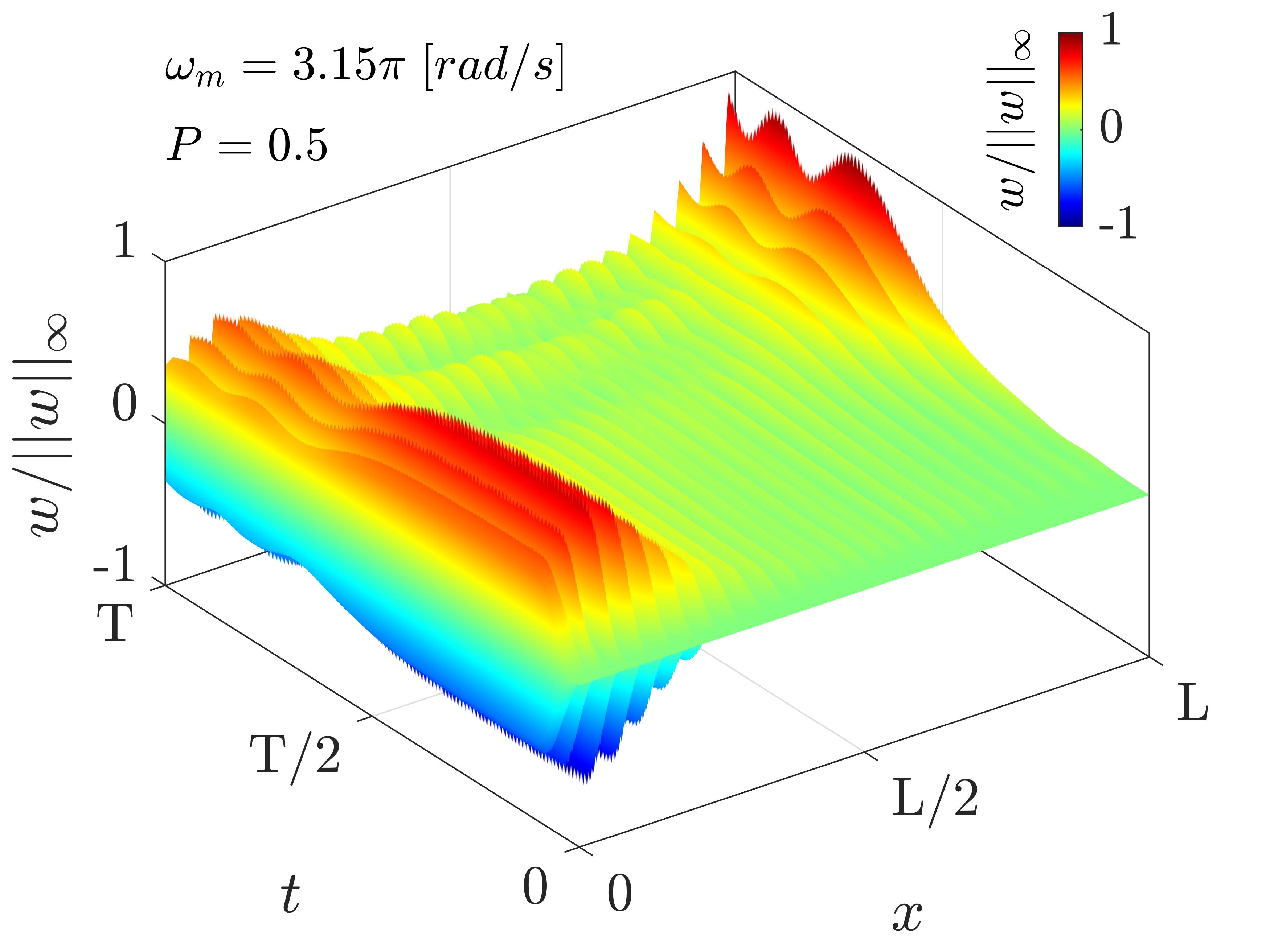
Now, based on the diabatic frequency estimation, the required modulation speed $\omega_{m}$ is evaluated as a function of the target steady-state transition probabilities $P$, the frequency separation $\Gamma_{CR}$, and the crossing slope $\gamma$, in agreement to Eq. 13. The estimated probabilities and modulation speeds are then validated numerically by solving the adiabatic and non-adiabatic transition problems. Specifically, a narrowband input spectrum, which is able to favor only the excitation of the left localized state, is considered. To this end, the shape of the input force is set coincident to the mode polarization ${\bm{w}}^{A}$ of the $25^{th}$ state computed for $\phi=\phi_{i}$. Later, the phase parameter is varied using three distinct values for $\omega_{m}=20\pi,\;3.15\pi,0.26\pi\;{\rm[rad/s]}$. The resulting displacement field is used to recover the energy content in reciprocal space $\hat{w}\left(f,\kappa_{x},t\right)$, which is then reduced to $\hat{w}\left(f,t\right)$, by taking the RMS value along $\kappa_{x}$. In case of fast modulation ($\omega_{m}=20\pi$), the probability for the initial state to keep the same polarization (i.e. to jump from $\Omega_{-}^{A}$ to $\Omega_{+}^{A}$ for $\phi_{CR}$) is $0.9$, which is confirmed by the associated spectrogram in Fig. 4(a). Consequently, the temporal evolution of the beam’s displacement (see Fig. 4(d)) illustrates that the topological state remains left localized (except for some energy that leaks to the right), which reflects the mode polarization ${\bm{x}^{A}}$ associated to the branch the solution belongs to. When the intermediate speed of $\omega_{m}=3.15\pi$ is applied to the system, corresponding to $P=0.5$, the energy content splits between two states which are left and right localized respectively, as shown in Fig. 4(b,e). Finally, a slow modulation, characterized by $\omega_{m}=0.26\pi$ and $P=2.4\cdot 10^{-4}$, results in a complete topological transitions from the left to right boundaries, therefore achieving a topological pump. The corresponding specrogram demonstrates that the topological transition occurs with a frequency shift, so that the initial state keeps belonging to the bottom branch with negligible scattering of energy to the neighboring modes.

In this manuscript it is demonstrated that the coupling between distinct topological states populating the same gap leads to the formation of avoided crossings characterized by edge-to-edge transitions. The avoided crossing dynamics is investigated in the context of quasiperiodic stiffness modulated beams and, specifically, we have shown a systematic procedure to break the modal coupling upon approximation of the diabatic frequencies and corresponding basis, which is used to estimate the required speed of modulation for a given edge-to-edge transition probability. The results presented in the paper can be of technological relevance for applications involving elastic energy splitting and demultiplexing, frequency conversion and waveguiding.

The authors wish to thank Dr. Massimo Ruzzene and M. Rosa for useful discussion in the preliminary stage of the present work.
The Italian Ministry of Education, University and Research is acknowledged for the support provided through the Project ”Department of Excellence LIS4.0 - Lightweight and Smart Structures for Industry 4.0”.

References

- Lu et al. (2014) L. Lu, J. D. Joannopoulos, and M. Soljačić, Nature Photonics 8, 821 (2014).
- Khanikaev et al. (2013) A. B. Khanikaev, S. H. Mousavi, W.-K. Tse, M. Kargarian, A. H. MacDonald, and G. Shvets, Nature materials 12, 233 (2013).
- Hasan and Kane (2010) M. Z. Hasan and C. L. Kane, Reviews of Modern Physics 82, 3045 (2010).
- Haldane (1988) F. D. M. Haldane, Physical review letters 61, 2015 (1988).
- Yang et al. (2015) Z. Yang, F. Gao, X. Shi, X. Lin, Z. Gao, Y. Chong, and B. Zhang, Phys. Rev. Lett. 114, 114301 (2015).
- Fleury et al. (2016) R. Fleury, A. B. Khanikaev, and A. Alu, Nature communications 7, 11744 (2016).
- Lu et al. (2017) J. Lu, C. Qiu, L. Ye, X. Fan, M. Ke, F. Zhang, and Z. Liu, Nature Physics 13, 369 (2017).
- Mousavi et al. (2015) S. H. Mousavi, A. B. Khanikaev, and Z. Wang, Nature communications 6, 8682 (2015).
- Huber (2016) S. D. Huber, Nature Physics 12, 621 (2016).
- Wang et al. (2015) P. Wang, L. Lu, and K. Bertoldi, Physical review letters 115, 104302 (2015).
- Nash et al. (2015) L. M. Nash, D. Kleckner, A. Read, V. Vitelli, A. M. Turner, and W. T. Irvine, Proceedings of the National Academy of Sciences 112, 14495 (2015).
- Souslov et al. (2017) A. Souslov, B. C. Van Zuiden, D. Bartolo, and V. Vitelli, Nature Physics 13, 1091 (2017).
- Chen et al. (2019) H. Chen, L. Yao, H. Nassar, and G. Huang, Physical Review Applied 11, 044029 (2019).
- Süsstrunk and Huber (2015) R. Süsstrunk and S. D. Huber, Science 349, 47 (2015).
- Pal et al. (2016) R. K. Pal, M. Schaeffer, and M. Ruzzene, Journal of Applied Physics 119, 084305 (2016).
- Chen et al. (2018) H. Chen, H. Nassar, A. N. Norris, G. K. Hu, and G. L. Huang, Phys. Rev. B 98, 094302 (2018).
- Miniaci et al. (2018) M. Miniaci, R. K. Pal, B. Morvan, and M. Ruzzene, Phys. Rev. X 8, 031074 (2018).
- Pal and Ruzzene (2017) R. K. Pal and M. Ruzzene, New Journal of Physics 19, 025001 (2017).
- Vila et al. (2017) J. Vila, R. K. Pal, and M. Ruzzene, Physical Review B 96, 134307 (2017).
- Liu and Semperlotti (2018) T.-W. Liu and F. Semperlotti, Physical Review Applied 9, 014001 (2018).
- Liu and Semperlotti (2019) T.-W. Liu and F. Semperlotti, Physical Review Applied 11, 014040 (2019).
- Riva et al. (2018) E. Riva, D. Quadrelli, G. Cazzulani, and F. Braghin, Journal of Applied Physics 124, 164903 (2018).
- Kraus and Zilberberg (2016) Y. E. Kraus and O. Zilberberg, Nature Physics 12, 624 (2016).
- Ozawa et al. (2016) T. Ozawa, H. M. Price, N. Goldman, O. Zilberberg, and I. Carusotto, Physical Review A 93, 043827 (2016).
- Lee et al. (2018) C. H. Lee, Y. Wang, Y. Chen, and X. Zhang, Physical Review B 98, 094434 (2018).
- Kraus et al. (2012) Y. E. Kraus, Y. Lahini, Z. Ringel, M. Verbin, and O. Zilberberg, Physical review letters 109, 106402 (2012).
- Zilberberg et al. (2018) O. Zilberberg, S. Huang, J. Guglielmon, M. Wang, K. P. Chen, Y. E. Kraus, and M. C. Rechtsman, Nature 553, 59 (2018).
- Apigo et al. (2019) D. J. Apigo, W. Cheng, K. F. Dobiszewski, E. Prodan, and C. Prodan, Physical review letters 122, 095501 (2019).
- Ni et al. (2019) X. Ni, K. Chen, M. Weiner, D. J. Apigo, C. Prodan, A. Alù, E. Prodan, and A. B. Khanikaev, Communications Physics 2, 55 (2019).
- Apigo et al. (2018) D. J. Apigo, K. Qian, C. Prodan, and E. Prodan, Physical Review Materials 2, 124203 (2018).
- Pal et al. (2019) R. K. Pal, M. I. N. Rosa, and M. Ruzzene, New Journal of Physics 21, 093017 (2019).
- Xia et al. (2020) Y. Xia, A. Erturk, and M. Ruzzene, Physical Review Applied 13, 014023 (2020).
- Brouzos et al. (2019) I. Brouzos, I. Kiorpelidis, F. Diakonos, and G. Theocharis, arXiv preprint arXiv:1911.03375 (2019).
- Verbin et al. (2015) M. Verbin, O. Zilberberg, Y. Lahini, Y. E. Kraus, and Y. Silberberg, Physical Review B 91, 064201 (2015).
- Nakajima et al. (2016) S. Nakajima, T. Tomita, S. Taie, T. Ichinose, H. Ozawa, L. Wang, M. Troyer, and Y. Takahashi, Nature Physics 12, 296 (2016).
- Lohse et al. (2016) M. Lohse, C. Schweizer, O. Zilberberg, M. Aidelsburger, and I. Bloch, Nature Physics 12, 350 (2016).
- Longhi (2019) S. Longhi, Physical Review B 99, 155150 (2019).
- Rosa et al. (2019) M. I. Rosa, R. K. Pal, J. R. Arruda, and M. Ruzzene, Physical Review Letters 123, 034301 (2019).
- Riva et al. (2020a) E. Riva, M. I. N. Rosa, and M. Ruzzene, Phys. Rev. B 101, 094307 (2020a).
- Grinberg et al. (2020) I. H. Grinberg, M. Lin, C. Harris, W. A. Benalcazar, C. W. Peterson, T. L. Hughes, and G. Bahl, Nature Communications 11, 1 (2020).
- Riva et al. (2019) E. Riva, J. Marconi, G. Cazzulani, and F. Braghin, Journal of Sound and Vibration 449, 172 (2019).
- Marconi et al. (2019) J. Marconi, E. Riva, M. Di Ronco, G. Cazzulani, F. Braghin, and M. Ruzzene, arXiv preprint arXiv:1909.13224 (2019).
- Riva et al. (2020b) E. Riva, M. Di Ronco, A. Elabd, G. Cazzulani, and F. Braghin, Journal of Sound and Vibration , 115186 (2020b).
- Nassar et al. (2018) H. Nassar, H. Chen, A. Norris, and G. Huang, Physical Review B 97, 014305 (2018).
- Marneffe and Preumont (2008) B. D. Marneffe and A. Preumont, Smart Materials and Structures, Vol. 17 (2008) p. 035015.
- Moheimani and Fleming (2006) S. R. Moheimani and A. J. Fleming, (2006).
- Fox and Kapoor (1968) R. Fox and M. Kapoor, AIAA journal 6, 2426 (1968).